A SIGMOIDAL MODEL FOR THE
INTERPRETATION OF QUANTITATIVE
PCR (qPCR) EXPERIMENTS
MODELO SIGMOIDAL PARA LA INTERPRETACIÓN DE
EXPERIMENTOS DE PCR CUANTITATIVO (qPCR)
Fecha de recepción: 10 de Julio de 2012•Fecha de aceptación: 22 de octubre de 2012
Pablo Andrés Gutiérrez Sánchez1 • Verónica Rodríguez Fuerte2 • Mauricio Marín Montoya3,4
ABSTRACT
Real-time or quantitative PCR (qPCR) is the most commonly used technique for estimating the amount of starting nucleic acids in a PCR or RT-PCR reaction. Quantification of PCR product is achieved in real time by measuring the increase in fluorescence of intercalating dyes, labeled primers or oligonucleotides in the pre-sence of double stranded DNA. This amplification curve follows a sigmoid behavior and is used to estimate the relative and/or absolute amount of template using different methods and assumptions. Estimation of C0
normally requires the measurement of a threshold cycle and some assumption about the efficiency of the reaction. An accurate estimation of efficiency is paramount for a precise determination of template levels at time zero. Several non-linear fitting methods have been implemented to model the sigmoid behavior using different empirical models with varying amounts of parameters; however, interpretation of the corresponding parameters is not straightforward. In this paper a model of PCR amplification is deduced and used in the inter-pretation of qPCR experiments. A non-linear regression analysis of this equation gives a direct estimation of
C0 and automatically calculates a parameter k related to the reaction efficiency. This model takes into account non-idealities in the amplification reaction and avoids a priori assumptions about efficiency.
Key words: qRT-PCR, non-linear regression, sigmoidal model
1 Associate Professor, Laboratory of Industrial Microbiology, Facultad de Ciencias, Universidad Nacional de Colombia Sede Medellín. paguties@unal.edu.co
2 Research Assistant, Laboratory of Industrial Microbiology, Facultad de Ciencias, Universidad Nacional de Colombia Sede Medellín. verodriguezf@gmail.com
3 Associate Professor, Laboratory of Cell and Molecular Biology, Facultad de Ciencias, Universidad Nacional de Colombia Sede Medellín. mamarinm@unal.edu.co
RESUMEN
La técnica de PCR en tiempo real (qPCR) es el método experimental más ampliamente utilizado para la determinación de la concentración inicial de ácidos nucleicos molde (C0 ) en reacciones de PCR o RT-PCR. La cuantificación de la cantidad de producto se mide a partir del incremento en la fluorescencia de agentes inter-calantes, cebadores u oligonucleótidos marcados e incorporados en el ADN de doble cadena. La estimación de C0 se lleva a cabo mediante la medición de un ciclo umbral de fluorescencia y algunas asunciones sobre la eficiencia de la reacción. Una correcta estimación de la eficiencia es fundamental para una determinación pre-cisa de las concentraciones iniciales de molde. Por esta razón, se han desarrollado algunos modelos empíricos del comportamiento sigmoidal de la reacción de amplificación; sin embargo, la interpretación de parámetros no corresponde necesariamente a aspectos específicos de la reacción. En este trabajo se deduce un modelo de la amplificación por PCR útil para la interpretación de experimentos de qPCR. La regresión no lineal de esta ecuación sobre datos experimentales permite obtener una estimación directa de C0 y arroja un parámetro k relacionado con la eficiencia de la reacción. Este modelo tiene en cuenta no idealidades en la amplificación y evita asunciones a priori sobre la eficiencia de la reacción.
Palabras clave: qRT-PCR, modelo sigmoidal, regresión no lineal
INTRODUCTION
Real-time or quantitative PCR (qPCR) is the most commonly used technique for estimating the amount of starting nucleic acids in a PCR or RT-PCR reaction. qPCR has become an indispensable tool in the assessment of transcription levels, determination of pathogen concentrations and detection of single nucleotide polymorphisms (SNPs) (Bustin, 2000; Hugget et al., 2004; VanGuilder et al., 2008). Quan-tification of PCR product is achieved in real time by measuring the increase in fluorescence of interca-lating dyes, labeled primers or oligonucleotides in the presence of double stranded DNA. The amount of initial template is estimated by determining the number of amplification cycles required to get a tar-get fluorescence level and the resulting amplification curve used to calculate the relative and/or absolute
amount of template using different methods and as-sumptions (Bustin, 2000). In an ideal situation, the number of copies would double after each ampli-fication cycle; however, because of several experi-mental factors this is normally not the case. Due to a limited amount of reagents, the PCR amplification process follows a sigmoidal behavior characterized by three phases (Bustin et al., 2005). During the lag phase, amplification kinetics is slow and without any noticeable increase in fluorescence compared to the background. In the exponential phase, there is a per-ceptible increase of fluorescence, which follows an exponential behavior and is typically the most use-ful data in qPCR experiments. Finally, a plateau is reached where no further amplification occurs due to exhaustion of reagents.
Estimation of the initial amount of template,
C0, requires the measurement of a threshold cycle where fluorescence rises significantly above the background level and some assumptions about the efficiency of the reaction. It is typically assumed that after the lag phase the amplification reaction is ex-ponential, but unfortunately this behavior only ap-plies when primers and reagents are not limiting. In traditional analysis, the efficiency of the amplification reaction ranges between a value of two for a perfect amplification and one when no amplification occurs (Pfaffl, 2001). An accurate estimation of efficiency is paramount for a precise determination of template
levels at time zero; this can be done empirically from the slope of a calibration curve at different DNA con-centrations (Livak & Schmittgen, 2001). However, ef-ficiency can vary significantly depending on the pres-ence of contaminants, PCR inhibitors and pipetting errors among other factors; to facilitate the analysis, test and control samples are assumed to have equal efficiencies. In the ∆,∆Ct method, a very popular procedure, efficiency is not even measured and is assumed to be close to the ideal case (~2.0), (Livak & Schmittgen, 2001). Another method estimates ef-ficiency from a linear fit to the exponential phase of each amplification curve avoiding the necessity of building a calibration curve, which results in a more
accurate estimation of individual efficiencies (Peirson
et al., 2001). As an alternative, several non-linear
fit-ting methods have been implemented to model the sigmoid behavior using empirical models with vary-ing amounts of parameters (Liu & Saint, 2002; Spiess
et al., 2002; Guescini et al., 2008; Rutledge & Stewart,
2008; Liu et al., 2011). Unfortunately, interpretation of the corresponding parameters is not straightfor-ward. A more accurate model should account for primer consumption and the sigmoidal behavior of the amplification reaction. In this paper a model of PCR amplification is deduced and used in the inter-pretation of qPCR experiments. A non-linear
regres-sion analysis of this equation gives a direct estima-tion of relative and initial concentraestima-tion of template and automatically calculates a parameter related to the reaction efficiency. This model takes into ac-count non-idealities in the amplification reaction and avoids any a priori assumptions about efficiency.
MATERIALS AND METHODS
Primers pairs EF1qF (5’-ACC CAG CAA AGG GTG CTG CC-3’, Tm=62.9 C) and EF1qR (5’-GGG AGG TGT GGC AGT CGA GC-3’, Tm=61.4 C) were designed to amplify a region of 104 bp of
Sola-num phureja elongation factor EF1A. qPCR assays
A model of PCR amplification is deduced and used in the
interpretation of qPCR experiments. This model takes into
account non-idealities in the amplification reaction and avoids
any a priori assumptions about efficiency.
were carried out in a Rotor-Gene Q real-time cycler (QIAGEN, Germany) using a Maxima SYBR Green/ Rox qPCR Master Mix kit (Thermo Scientific, EEUU) following the manufacturer’s protocol. Dilutions 1:1, 1:10, 1:100 and 1:1000 of a DNA amplicon at 123.4 ng/µl were used as template in the qPCR experiments. For each sample, 4.5 µl ddH20, 6.3 µl mix, 0.35 µl (10 µM) of each primer and 1 µl of DNA solution was added to the reaction mixture in a final volume of 12.5 µl. Reaction mixtures were incubated for ten minutes at 95 °C and followed by 30 amplification cycles of 15 s at 95°C and 1 min at 60°C. Four repetitions per sample and a no-tem-plate control were run.
Melting curve and gel electrophoresis of the amplification products were employed to confirm the presence of an unique amplified product of ex-pected size (data not shown). Threshold values for each qPCR reaction were set at 0.5 and 1.0 units of fluorescence; efficiencies were estimated from the slope at the exponential phase using the method described by Peirson et al. (2001). Nonlinear regres-sion of qPCR data was performed with the Leven-berg-Marquardt method using a custom Matlab script (Ahearn et al., 2005).
RESULTS AND DISCUSSION
Derivation of the amplification model
The polymerase chain reaction can be modeled as a bimolecular reaction between template and primers with kinetic constant k. This constant deter-mines the reaction rate and can be interpreted as a measure of reaction efficiency that encompasses all non-idealities. As the sum of template and primer concentration is constant, the kinetics of the PCR re-action can be represented by the following differen-tial equation:
Where C and P represent the concentration of template and primers respectively; Cm is the sum of C and P and corresponds to the maximum amount of DNA that can be produced in the PCR reaction. Solu-tion of this differential equaSolu-tion results in a formula describing de time-dependent variation of DNA concentration:
Where C0 is template concentration at time 0 which is the value of interest in qPCR experiments and B an arbitrary integration constant.
The effects of each parameter on the amplifica-tion curve are shown in Figure 1. Variaamplifica-tions on initial concentration only affect the position of the ampli-fication curve along the x-axis but do not affect the slope at a fixed concentration value (Fig. 1A). This is the ideal situation for accurate estimation of C0 us-ing threshold cycles of amplification. Unfortunately, variations of k and/or Cm can have a dramatic effect on the estimation of the threshold cycle for samples with the same initial concentration of template (Fig. 1B, C). Variations of k can be due factors affecting the efficiency of the PCR reaction such as the pres-ence of inhibitors. Variations of Cm, on the other hand, can be attributed to pipetting errors that can limit the maximum amount of DNA obtained per sample. Unfortunately, it is a common practice to analyze qPCR experiments using only thresh-old cycles with dismissal of the remaining data in the amplification curve. With traditional methods,
C0 will be underestimated for samples with low ef-ficiency if corrections are not taken into account. A similar situation arises when samples reach dif-ferent final DNA concentrations. Our model can discriminate between slow amplification due to in-hibition of the PCR reaction by limited amount of reagents, variations of efficiency and/or low tem-plate concentration. = kCP = kC (Cm-C) [1] C6 t6 Cm C0 e ktCm Cm + C0 (e ktCm -1) C (t) = B + [2]
Application to the analysis of experimental data
To test the accuracy of proposed model, a qPCR experiment was performed using four dilutions of template (1:1, 1:10, 1:100 and 1:1000) with four replicates. Experimentally, the amount of DNA pro-duced during the amplification reaction is moni-tored using either fluorescent probes or DNA-bind-ing fluorophores such as SYBR green (VanGuilder et al., 2008). It is assumed that the amount of dsDNA present in the sample is proportional to the amount of fluorescence. Therefore, equation [2] must be ex-pressed in terms of fluorescence and include cor-rections due to non-zero baseline and fluorescence drift over time:
Fn=An+Fb+ F0∆Fenkƒ∆F
∆F+F0 (enkƒ∆F-1)
Where Fb and Fm correspond to baseline and maximum fluorescence, F0 is the fluorescence due to template concentration at the beginning of the amplification reaction and kf is a corrected kinetic constant expressed in terms of fluorescence units. A graphical representation of each parameter is presented in figure 2.
F0 values can used to estimate the relative tem-plate using the following expression:
Where Rij is the relative concentration of sample i
with respect to sample j, C0 and C0j are the template concentrations at time zero for samples i and j; F0i and
F0i is the fluorescence due to the template at time zero
Figure 1. Effect of parameters on the amplification curve. See text for details.
[3]
Figure 2. Graphical interpretation of parameters from the amplifica-tion curve. Concentration 10-2 10-6 10-10 10-14 C1 = 1 k = 1 0 10 20 30 40 Cycle number Cr = 1 C0 = 10-2 k=1 k=0.6 k=0.4 k=0.2 k=0.1 0 10 20 30 40 Ct = 1 Ct = 0.8 Ct = 0.6 Ct = 0.4 Ct = 0.2 C0 = 10-2 k = 1 0 10 20 30 40 Fluor escence Cycle number An+Fb Fm Fn ∆F ∆n Rij = = [4]C0 i C0 j F0 i F0 j
for samples i and j. An absolute measure of C0can be calculated using a standard sample with known C0 and multiplying by the relative concentration to the stan-dard. F0 can be estimated by a non-linear fit of equa-tion [3] to the experimental data, using initial estimates
A’, Fb’, ∆F’, F0’ and kf’ of the different parameters from the amplification curve. A’=0 is a good approxima-tion, in cases where the fluorescence change over time is not significant. A graphical representation of these estimators is shown in figure 2. Initial estimates of Fb and ∆F are Fb=Fmin and ∆F=Fmax-Fmin, where Fmax and
Fmin represent the maximum and minimum fluores-cence values during the amplification curve. An initial
* Parameters after non-linear fit to equation (3) using the Levenberg–Marquardt method with the initial parameters shown on the left.
estimate of k can be calculated using two adjacent data points Fn and Fn-1 in the exponential phase and substi-tuting them in the following equation:
An initial estimator of F0 can be obtaining explic-itly by substituting k’, Fb’, and ∆F into the expression:
Initial values of A, F0, k, Fb’, and ∆F for the experi-mental data are shown in table 1.
k'= (Fn-Fn-1) (Fn-F'b)(∆F'-Fn) [5] F0'= (Fn-Fb) ∆F ∆FenkƒDF-(F n-Fb)(enkƒDF-1) [6] Dilution
Initial Parameters Non-linear fit* DCt method
Fmin DF´ k´ F0´ A Fb DF k F0 (10RSS-2) Eff Ct (0.5) (1.0)Ct 1:1 0.72 2.31 0.34 8.91E-2 -0.05 0.09 3.58 0.15 4.17E-1 1.6 1.36 1 3 0.77 2.73 0.28 9.77E-2 -0.04 0.10 3.92 0.14 4.35E-1 4.1 1.37 1 2 0.76 2.77 0.26 1.15E-1 -0.05 -0.09 4.29 0.11 5.78E-1 1.6 1.37 1 2 0.71 2.22 0.32 1.10E-1 -0.05 0.04 3.48 0.15 4.55E-1 1.3 1.36 1 3 1:10 0.46 2.91 0.25 1.47E-2 -0.03 0.43 3.46 0.17 4.20E-2 2.7 1.36 4 6 0.45 2.84 0.25 1.56E-2 -0.03 0.38 3.50 0.16 5.77E-2 3.0 1.35 5 6 0.46 3.16 0.23 1.32E-2 -0.04 0.39 3.82 0.15 5.49E-2 2.7 1.36 4 6 0.48 2.88 0.26 1.16E-2 -0.03 0.43 3.43 0.17 4.31E-2 2.8 1.36 4 6 1:100 0.44 2.68 0.27 1.34E-3 -0.04 0.52 3.45 0.16 9.90E-3 2.0 1.37 8 9 0.45 4.33 0.15 3.99E-3 0.00 0.41 4.31 0.14 6.07E-3 5.1 1.41 7 8 0.43 3.11 0.22 3.09E-3 -0.03 0.48 3.66 0.16 10.1E-3 2.1 1.38 7 9 0.47 4.04 0.16 3.04E-3 -0.01 0.46 4.25 0.14 7.66E-3 5.7 1.38 7 9 1:1000 0.4 2.65 0.28 1.20E-4 -0.036 0.53 3.28 0.17 1.81E-3 4.1 1.36 11 12 0.38 4.8 0.12 1.40E-3 0.011 0.30 4.53 0.13 0.86E-3 11.7 1.45 11 12 0.39 2.17 0.34 9.96E-5 -0.032 0.51 2.71 0.21 1.21E-3 3.0 1.34 12 13 0.41 3.09 0.23 1.96E-4 -0.029 0.53 3.49 0.16 1.22E-3 3.7 1.38 11 12 Table 1. Parameters used in the estimation of relative concentrations by the different methods discussed in the text.
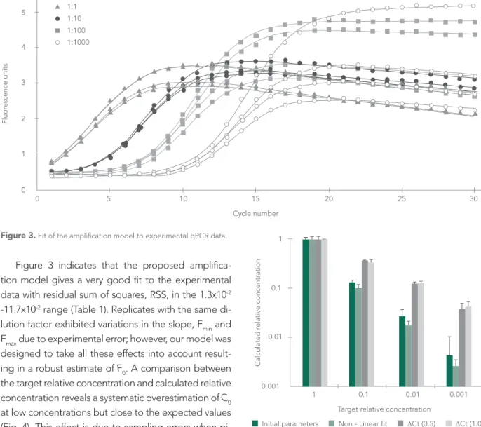
Figure 3 indicates that the proposed amplifica-tion model gives a very good fit to the experimental data with residual sum of squares, RSS, in the 1.3x10⁻²
-11.7x10⁻² range (Table 1). Replicates with the same
di-lution factor exhibited variations in the slope, Fmin and Fmax due to experimental error; however, our model was designed to take all these effects into account result-ing in a robust estimate of F0. A comparison between the target relative concentration and calculated relative concentration reveals a systematic overestimation of C0
at low concentrations but close to the expected values (Fig. 4). This effect is due to sampling errors when pi-petting low concentrated solutions and has been ob-served in similar studies on qPCR (Liu et al., 2011).
Surprisingly, good estimates of the relative con-centrations can also be obtained using the graphical estimates of A, k’, Fb’, and ∆F’ and substituting them into equation [6]. This is an alternative when non-linear fit to the data is not possible. As expected this meth-od is less accurate and shows a higher standard devia-tion of estimated relative concentradevia-tions as compared to those calculated using non-linear fit (Fig. 4).
Figure 3. Fit of the amplification model to experimental qPCR data.
Figure 4. Comparison of initial concentration predictions from various qPCR data analysis methods for gene EF1A.
Rij=
C0i
= (1+ej)nj [7]
C0j (1+ei)ni
Our method was contrasted with a previously re-ported procedure routinely used in the analysis of qPCR data (Livak & Schmittgen, 2001). This proce-dure uses the following formula for relative quantifi-cation between two samples:
Fluor escence units 1 2 3 4 5 5 10 15 Cycle number 20 25 30 0 0 1:100 1:10 1:1000 1:1
Target relative concentration
1 0.1 0.01 0.001
0.01 0.1 1
0.001
Initial parameters Non - Linear fit ∆Ct (0.5) ∆Ct (1.0)
Calculated r
Where ej and ei represent reaction efficiencies and nj and ni threshold cycles for each reaction. Effi-ciency was calculated using a procedure described by Peirson et al. (2003). This procedure requires the determination of a cycle n where fluorescence reaches a given threshold value and an estimation of reaction efficiency using a linear fit of the loga-rithmized data within the exponential region of the amplification curve. Estimates of relative concentra-tion were calculated using two thresholds of fluo-rescence: 0.5 and 1.0. Relative concentrations were estimated relative to the average cycle number and efficiency for the sample without dilution. Thresh-old cycles and efficiencies are reported on table 1. These calculations reveal that the ∆Ct method de-viates significantly from the known concentrations as shown in figure 4. The biggest source of errors probably lies in the assumption that the PCR re-action is exponential, a well-known issue in qPCR analysis. This can be clearly seen when comparing the average deviation to the target concentrations shown in Table 2. The lowest deviations were ob-tained with relative concentrations calculated using the non-linear fit method here proposed with val-ues in the -1.71-0 range. Estimates using the initial guesses deviated a little more with values between -1.71 and zero. Percent deviations were about an order of magnitude higher using the Ct method when compared with estimates from the non-linear method: -36.31 to 0 using a threshold value of 0.5 and -36.31 to 0 for the 1.0 threshold.
Several sigmoidal models have been developed to fit PCR data such as the Boltzmann and logistic function (Pfaffl, 2001; Mehra & Hu, 2005; Rebrikov & Trofinov, 2006; Ritz & Spiess, 2008). Fitting of these equations allows a more accurate determination of threshold cycles and efficiency and avoids the construction of standard curves. Unfortunately, the empirical nature of these models makes it difficult to interpret parameters in terms of experimental
variables. Even worse, relative concentrations are calculated using classical methods that assume the amplification process to be exponential. Contrary to previous models, ours is deduced from first prin-ciples and each parameter can be given a direct ex-perimental interpretation, which can also be used to facilitate the interpretation of qPCR runs.
CONCLUSION
The proposed method gives a better perfor-mance at determining relative concentration in qPCR experiments as compared to the widely used Ct method. In contrast to other empirical sigmoidal models, ours is deduced from first principles and each parameter can be interpreted in terms of ex-perimental events.
ACKNOWLEDGEMENTS
This work was supported by Vicerrectoría de Investigaciones de la Universidad Nacional de Co-lombia. Grant: 20101009932. Convocatoria Nacional para el fortalecimiento de los Grupos de Investig-ación y CreInvestig-ación Artística de la Universidad Nacional de Colombia. 2010-2012.
*Percentage deviations were calculated using the relation 1
00(Ev-Ov)/Ev where EV and Ov are the Expected and Observed values, respectively.
Dilution ParametersInitial Linear fitNon- (0.5)DCt (1.0)DCt
1:1 0.0 0.0 0.0 -0.01
1:10 -0.34 -0.05 -2.75 -2.48
1:100 -1.78 -0.79 -11.99 -11.68
1:1000 -3.41 -1.71 -36.37 -42.42
Table 2. Percentage deviations for initial concentration estimates with the qPCR analysis methods discussed in the text*.
REFERENCES
1. Ahearn TS, Staff RT, Redpath TW, Semple SI. 2005. The use of the Levenberg-Marquardt curve-fitting algorithm in pharmacokinetic mo-delling of DCE-MRI data. Physics in Medicine and Biology. 50:N85-92.
2. Bustin SA. 2000. Absolute quantification of mRNA using real-time reverse transcription polymerase chain reaction assays. Journal of Molecular Endocrinology, 25:169-93.
3. Bustin SA, Benes V, Nolan T, Pfaffl MW. 2005. Quantitative real-time RT-PCR – a perspective. Journal of Molecular Endocrinology, 34:597-601. 4. Hugget J, Dheda K, Bustin S, Zumla A. 2005.
Real-time RT-PCR normalization; strategies and considerations. Genes and Immunity, 6:279-284.
5. Guescini M, Sisti D, Rocchi MB, Stocchi L, Stocchi V. 2008. A new real-time PCR method to overcome significant quantitative inaccura-cy due to slight amplification inhibition. BMC Bioinformatics, 9:326.
6. Liu W, Saint DA. 2002. Validation of a quan-titative method for real-time PCR kinetics.
Biochemical and Biophysical Research Com-munications, 12:1047-1064.
7. Liu M, Udhe-Stone C, Goudar CT. 2011. Pro-gress curve analysis of qRT-PCR reactions using the logistic growth equation. Biotechnol Pro-gress, 27:1407-1414.
8. Livak KJ, Schmittgen TD. 2001. Analysis of
re-lative gene expression data using real-time quantitative PCR and the 2(-Delta Delta C(T)) method. Methods, 25:402-408.
9. Mehra S, Hu WS. 2005. A kinetic model of quantitative real-time polymerase chain reac-tion. Biotechnology and Bioengineering, 91:848-860.
10. Peirson SN, Buttler JN, Foster RG. 2001. Expe-rimental validation of novel and conventional approaches to quantitative real-time PCR data analysis. Nucleic Acids Research, 29:e45. 11. Peirson SN, Butler JN, Foster RG. 2003.
Expe-rimental validation of novel and conventional approaches to quantitative real-time PCR data analysis. Nucleic Acids Research 31:e73.
12. Pfaffl, MW. 2001. A new mathematical model for relative quantification in real-time RT-PCR. Nucleic Acids Research, 29:e45
13. Rebrikov DV, Trofinov DY. 2006. Real-Time PCR: A Review of approaches to data analy-sis. Applied biochemistry and microbiology, 42:455-463.
14. Ritz C, Spiess AN. 2008. qPCR: an R package for sigmoidal model selection in quantitative real-time polymerase chain reaction analysis. Bioinformatics, 24:1549-1551.
15. Rutledge RG, Stewart D. 2008. A kinetic-based sigmoidal model for the polymerase chain reaction and its application to high-capacity absolute quantitative real-time PCR. BMC Bio-technology, 8:47.
16. Spiess AN, Feig C, Ritz C. 2008. Highly accu-rate sigmoidal fitting of real-time PCR data by introducing a parameter for asymmetry. BMC Bioinformatics, 9:221.
17. VanGuilder HD, Vrana KE, Freeman WM. 2008. Twenty-five years of quantitative PCR for gene expression analysis. BioTechniques, 44:619-626.