1
An Introduction to Personal Network Analysis
and Tie Churn Statistics using E-NET
Daniel S. Halgin & Stephen P. Borgatti LINKS Center for Social Network Analysis
Gatton College of Business & Economics University of Kentucky
Lexington, KY 40506
Contact info danhalgin@uky.edu
ACKNOWLEDGEMENTS: The authors are grateful to the Connections editorial team and members of the LINKS Center for social network analysis at the University of Kentucky, especially Dan Brass, Joe Labianca, and Ajay Mehra for their help in shaping our thinking. This work was funded in part by the grant “Detection, Explanation and Prediction of Emerging Network Developments (DEPEND)” DARPA.
2
An Introduction to Personal Network Analysis
and Tie Churn Statistics using E-NET
Abstract
In this article we review foundational aspects of personal network analysis (also called ego network analysis) and introduce E-NET (Borgatti 2006), a computer program designed specifically for personal network analysis. We present the basic steps for personal network data collection and use E-NET to review key measures of personal network analysis such as size, composition and structure. We close by introducing longitudinal measures of personal network change, including tie churn, brokerage elasticity, and triad change. We argue that these measures can help reveal change patterns consistent with tie formation strategies that would otherwise be missed using more traditional analytic approaches.
3 Table of Contents
1. Introduction
2. Data collection in personal network research designs 3. Analysis of Personal Network Data using E-NET
1. Importing personal network data into E-NET 1.Row-wise format
2.Column-wise format 3.Full network format 2. Data Organization in E-NET
1.Egos tab 2. Alters
3.Alter-alter ties 4.Visualization 5.Measures 3. Data Analysis in E-NET
1.Compositional 2.Structural 4. Data Filtering
4. Longitudinal Analysis and Tie Churn Statistics 5. Conclusion
1. Introduction
In this article we introduce E-NET (Borgatti 2006), a software package specifically designed for the analysis ego network data (as opposed to "whole-network" data), and in particular ego network data collected via a personal network research design (PNRD1). In presenting the capabilities of the program, we review key ideas in the analysis of ego network data, and discuss specific measures used to describe the size, composition, and structure of personal networks. We close with new directions in the analysis of such data focusing on longitudinal analysis.
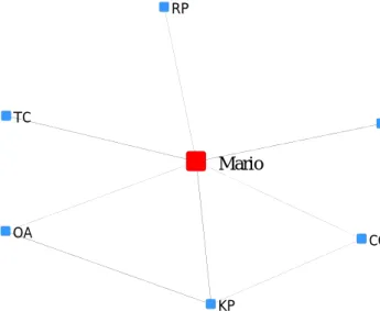
An ego network consists of a focal node ("ego"), together with the nodes they are directly connected to (termed "alters") plus the ties, if any, among the alters, as shown in Figure 1.
1
4
Figure 1. Ego network of Mario
These networks are also known as personal networks, ego-centric networks, and first order neighborhoods of ego (cf Everett & Borgatti, 2005; Mitchell 1969; Wellman, 1979). Ego networks may be obtained by extracting them from a full network, as illustrated in Figure 2 (Holly’s ego network is extracted from the full network). In that case (that is, when the full network is available), the decision to analyze just the ego networks is a theoretical choice to focus on the local rather than the global.
TC DK RP CC Mario OA KP
5
Figure 2. Extraction of Holly’s ego network from a full network
Ego networks may also be collected directly, using a personal network research design or PNRD. A PNRD involves sampling a collection of unrelated respondents (called egos) and asking them about the people in their lives (called alters). For example, if we are interested in the social factors that influence entrepreneurial success, a personal network research design would involve sampling a set of unrelated entrepreneurs and ask each one about the resources that they derive from their personal contacts. We could easily interview entrepreneurs in different countries and relate aspects of their networks with some chosen dependent variable such as firm performance or funds collected. Although we sacrifice the ability to analyze global network measures, the personal network approach allows us to investigate whether successful entrepreneurs tend to have a greater number of contacts than others, whether entrepreneurs in New York tend to have a more diverse set of personal networks than those in Rome, or whether male entrepreneurs tend to have more personal contacts who run in different social circles than female entrepreneurs. We might also use the personal network approach to conduct an in-depth analysis of one focal entrepreneur.
In this example, it seems like the PNRD has advantages over the alternative design, the full network research design (FNRD). In a full network research design, we begin with a set of nodes, then measure all of the ties of a given type among those nodes. So in the study of entrepreneurs, the first
HOLLY BRAZEY CAROL PAM PAT JENNIE PAULINE ANN MICHAEL BILL LEE DON JOHN HARRY GERY STEVE BERT RUSS HOLLY PAM PAT MICHAEL DON HARRY
6
design decision would be to determine which nodes to study. A natural first attempt would be to take as our nodes a set of entrepreneurs, such as all entrepreneurs belonging to a given association of
entrepreneurs. But the people from whom entrepreneurs obtain key resources need not be other
entrepreneurs. They could be friends, family, rich widows, and so on, who would probably not be in our population. A second attempt might be to study the whole of a small community in which there were entrepreneurs but also sources for these entrepreneurs, and we would measure ties among all pairs of nodes. This would yield very rich data, but could get enormous very fast, and much of the data might not be directly relevant to our research question. If we also wanted to compare New York and Rome
entrepreneurs, we would have double the size of our study.
In summary, sometimes we will find it useful to collect our ego network data using a PNRD rather than an FNRD. If so, however, we will find that the data resulting from PNRDs are quite different from those generated by FNRDs, and computer programs designed to analyze full network data, such as UCINET (Borgatti Everett & Freeman 2002) will have significant difficulty coping with the FNRD data. This is the need filled by specialized PNRD software such as E-NET, presented here, and other programs such as EgoNet (McCarty 2003).
2. Data Collection in Personal Network Research Designs
In the personal network research design (PNRD), researchers collect network data by sampling unrelated and anonymous respondents from a large population and gathering information about each of their ego networks. A personal network survey can be administered by interviewers, or given to respondents to fill out, either on paper or via online methods.
The typical first step of the PNRD is to generate an exhaustive list of alters with whom the respondent has some type of relationship. Termed a name generator, the respondent might be asked to list alters who occupy certain social roles (e.g., neighbors, kin, friends, coworker), those with whom he shares interactions (e.g., discuss important matters with, has sex with, etc.), or those with whom he exchanges flows (e.g., borrowed money from, provide emotional support to). This approach is used in many classic studies of personal networks (e.g., Burt 1984; Fisher 1982; Lauman 1966 1973; Wellman 1979). The
7
open-ended nature of name generators can result in lengthy surveys so scholars should be aware of order-effects, fatigue, satisficing, non-redundancy, as well as interviewer effects (Marsden 2003; Pustejovsky & Spillane 2009; Van Tilberg 1998). If faced with time constraints the researcher might limit the number of alters that each ego can nominate: “If you look back over the last six months, who are the four or five people with whom you discussed matters important to you?” (Burt 1984)2. Or, the researcher might focus the name generator question to best match the specific line of research: “Among the people with whom you work, who has provided you with emotional support in the past six months?” Other name generator approaches include the reverse-small-world instrument (Killworth et al., 1984), the phone book technique (e.g., Poole & Kochen 1978; Freeman & Thompson 1989), the modified multiple generator (MMG) and multiple generator random interpreter (MGRI) (Marin & Hampton 2007), as well as techniques that incorporate visual interfaces (e.g, Kahn & Antonucci 1980; McCarty & Govindaramanujam 2006).
After obtaining a list of names using name generator questions, the researcher then typically asks the respondent name interpreter questions. These questions elicit additional information about ego’s perceptions of the attributes of each alter (e.g., sex, race, income, etc.) and the shared relationship (e.g., duration, intensity, frequency, etc.). See Figure 3 for an example of a name interpreter grid. Name interpreter questions are unique to the PNRD and further highlight the ego-centered nature of this approach (as opposed to a full network design). Specifically, it is ego (not the alters) who provides information about the attributes of each alter. Researchers using a pure PNRD do not contact nominated alters to confirm alter attribute and relationship data and frequently use an alter-naming typology that allows ego to differentiate among alters without identifying them too closely (e.g., initials, code names, first three initials of first name and last name, etc.). This reduces privacy issues such as the lack of
anonymity of alters in the full network approach and can be more favorable for respondents3. In addition, the key focus of personal network research is the ego-centered world of each respondent and how she
2
For a more detailed discussion of personal network size and how the number of alters can influence analytic options see the work of Killworth (et al., 1990), and McCarty (et al., 2001, 2002).
3
The researcher might also consider a partial network research design using a snowball sampling method of contacting alters nominated by ego.
8
views her alters (i.e., the number of alters, alter attributes, relationship attributes, the presence of relationships among alters, etc.). One limitation of the PNRD approach is that we do not check the accuracy of ego’s view of his network (e.g., whether ego actually has ties with the nominated alters). In addition, we cannot fully determine the availability of all possible alters in ego’s world. With full networks we have a bounded study population and can thus analyze whether certain individuals have more ties than expected to alters with certain attributes, say members of the same gender. With personal networks, we only see the world through ego’s eyes so we don’t know who ego chooses not to connect with. Consider the case where one of our entrepreneurs almost exclusively named alters who are male. The personal network approach does not allow us to determine whether the respondent consciously chooses to avoid women or if he lives in a community (e.g., Silicon Valley) with a highly unbalanced gender ratio and therefore has limited opportunities to nominate women.
Ego ID Alter ID Alter Age Alter Gender Alter Religion Alter Income Alter frequency of contact
Mario RP 32 Male Muslim 55000 4
Mario CC 18 Female Catholic 23000 1
Mario OA 28 Female Catholic 64000 4
Mario TC 56 Male Protestant 43000 2
Mario KP 31 Male Muslim 17000 2
Figure 3. Name interpreter grid for Ego Mario
Depending on the research goals, the researcher might also ask name interrelator questions that require the respondent to indicate whether the nominated alters themselves are connected. Due to time constraints and to avoid respondent fatigue, name interrelators typically use a reduced set of alters from the name generator (e.g., 10 alters) and one specific alter-alter relationship such as whether or not the alters know each other. Figure 4 is an example of a name interrelator matrix that might be given to the respondent. The alter identifiers in the matrix (in this case, initials) must be consistent with the identifiers of a set of alters that ego nominated in the name generator.
9 RP CC OA TC KP RP CC 0 OA 0 0 TC 0 0 0 KP 0 1 1 0 Figure 4. Name Interrelator Matrix for Mario’s Ego Network
In summary, there are pros and cons of the PNRD as presented in table 1. For additional discussion of issues associated with the PNRD see Borgatti, Everett and Johnson (2013).
Pros Cons
Able to sample respondents at random and generalize to well-specified populations
Studies are scalable. Data storage and computing time requirements increase essentially linearly with the number of respondents, unlike whole network designs
Allows anonymity of respondents and alters,
reducing privacy issues and promoting response rates
Data do not have statistical issues such as lack of independence that must be addressed when analyzing full network data
Difficult to determine the availability of possible alters in ego’s world
Data contain only nominations by ego -- the choice to not nominate someone is not observed Alter-alter ties are as perceived by ego, and may be inaccurate
Inability to confirm ties (e.g., by looking at alter’s response about ego)
Asking ego to report on every alter can be very time intensive
Table 1. Pros and Cons of the PNRD 3. Analysis of Personal Network Data using E-NET
Once collected, personal network data can be organized and analyzed using E-NET (Borgatti 2006), a free program that specializes in the analysis of ego network data, particularly data obtained via personal network research design. E-NET accepts data pertaining to egos (e.g., age, sex), alters (e.g., relationship between ego and alter, alter attributes), and relationships among the alters (e.g., whether ego 1 reports that alter A is connected with alter B). Other tools for the analysis of ego network data include VennMaker (Gamper et al., 2012) and EgoNet (McCarty 2003). VennMaker uses a visual interface that allows ego to move alters around the screen to elicit both the types of relations and their strengths. EgoNet uses a computer interface that elicits ego data from respondents using questions that achieve both
10
name generation and interpretation. The program allows for visualization of ego networks, data management in a SPSS format, and a suite of standard network measures. In addition, Sciandra, Gioachin, and Finos (2012) provide an R package specific to the analysis of ego network data, and Müller, Wellman, and Marin (1999), provide guidelines for analyzing ego network in SPSS (For a discussion of additional options for the analysis and visualization of ego network data see McCarty et al., 2007).
3.1Importing personal network data to E-NET
Personal network data can be imported into E-NET in two formats, which we term row-wise, and column-wise. E-NET also reads full network data.
3.1.1 Row-wise format
In the row-wise format, data are recorded as three matrices corresponding to ego, ego-alter relationships, and alter-alter relationships4. The first matrix contains the collected attributes about each ego surveyed. The rows correspond to egos and the columns correspond to collected attributes about each ego. In the sample matrix provided in Figure 5, Ego 2 is a 30 year old woman with an income of 85000.
ID Age Sex Income
1 21 Male 18000
2 30 Female 85000
3 45 Female 32000
Figure 5. Ego data matrix
The second matrix (see Figure 6) contains information about ego-alter relationships. These data include attributes of ego’s relationship(s) with each alter (i.e., presence/absence, strength, frequency, etc.) as well as ego’s perception of each alter. Note that each row of the matrix corresponds to ego’s
relationship with a unique alter. Egos with multiple alters will have multiple rows of data. If the researcher collects data about multiple kinds of relationships with each alter, the additional relationships
4
We recommend that users first create the three matrices in Excel (or a similar program) and then compile into one document as discussed below.
11
are captured by added columns. In the sample matrix, Ego 1 has both a friendship and mentorship tie to alter 1_1, a friendship tie to alter 1_2, and a mentorship tie to alter 1_3. For convenience, we have used labels for the alters that include a reference to the ego they are attached to, hence alter “1_3” is the third alter of ego 1. The alter data matrix also includes the attributes of each alter (from ego’s point of view). For example, alter 1_1 is a 40 year old woman, at least according to ego.
From To Friend Mentor Alter Age Alter Sex
1 1_1 1 1 40 Female 1 1_2 1 0 33 Male 1 1_3 0 1 42 Female 2 2_1 0 1 63 Male 3 3_1 1 1 43 Female 3 3_2 1 1 21 Female
Figure 6. Alter data (row-based format)
As shown in Figure 7, the third matrix contains information about ego’s perceptions of the presence of relationships (if any) among alters. The first two columns are the IDs of the alters that have a tie. For example, rows 1 and 2 of Figure 7 indicate that Ego 1 reports that Alter 1(1_1) knows both Alter 2 (1_2) and Alter 3 (1_3).
From To Knows
1_1 1_2 1
1_1 1_3 1
Figure 7. Alter-alter data (row-based format)
When ready for importation into ENET, the user compiles the three matrices into a single text file using the VNA format (See Figure 8 for an example). The VNA file can be created by copy-and-pasting the matrices from a spreadsheet editor (e.g., Excel) into any text editor (e.g., Notepad) and saving the document with file extension .vna. Note that in the VNA file the three kinds of data are identified by an asterisk and matrix title (“*ego data”, “*alter data”, “*alter-alter data”).
*ego data
ID Age Sex Income 1 21 Male 18000 2 30 Female 85000 3 45 Female 32000
12 *alter data
From To Friends Mentor Age Sex 1 1_1 1 1 20 Female 1 1_2 1 0 33 Male 1 1_3 0 1 24 Female 2 2_1 0 1 63 Male 3 3_1 1 1 43 Female 3 3_2 1 1 21 Female *alter-alter data From To Knows 1_1 1_2 1 1_1 1_3 1
Figure 8. Row-based VNA file format
3.1.2 Column-wise format
E-NET also reads personal network data organized in an Excel file in what we term the column-wise format (see Figure 9). In this approach, the data are organized in one matrix such that each row corresponds to a specific respondent (ego) and columns correspond to ego attributes, ego-alter ties and perceptions, and alter-alter relationships. Note that the alter variables across the columns are repeated for each alter and labeled such that either the variable name is preceded by the alter number (e.g., A1Age, A2Age, A3Age, A1Sex, A2Sex, A3Sex) or vice versa (e.g., Age1 Age2 Age3 Sex1 Sex2 Sex3). Variables capturing ties among alters are named using the following format: “<variable name> <alter number> - <alter number>” (e.g., “knows1-2” indicates that alter1 knows alter 2). Using this naming convention enables E-NET to automatically identify ego variables, ego-alter ties and perceptions, and alter-alter ties. (If a different naming convention is used, the user can manually identify the variables by type within E-NET).
Age Sex Income A1Age A2Age A3Age A1Sex A2Sex A3Sex A1Friend A2Friend A3Friend knows1-2
21 Female 18000 20 33 24 Female Male Female 1 1 1 1
30 Male 85000 63 Male 0 0
13
Figure 9. Column-wise data format 3.1.3 Full network
E-NET also accepts full network data (i.e., sociometric data) stored in the UCINET data file format5. The analysis of full network data using E-NET is appropriate when the researcher is only interested in ego-centric measures. For instance, one might import the full network data presented in Figure 2 and use E-NET to extract, analyze, and compare the ego network of Holly with the ego networks of the other 17 individuals in the full network.
3.1.4 Importing the data
Once the data are properly organized into a row-wise (vna file), column-wise (excel file), or full network data format (UCINET file), the appropriate file can be imported into E-NET under File | Open. 3.2 Data Organization in E-NET
In discussing the organization of the program, we use data from the 1985 General Social Survey (GSS) as a running example. The GSS is a personal-interview survey designed to monitor changes in both social characteristics and attitudes currently being conducted in the United States. In 1985, the survey included a selection of personal network questions based on the following name generator:
From time to time, most people discuss important matters with other people. Looking back over the last six months- who are the people with whom you discussed matters important to you? Just tell me their first names or initials.
Name interpreter questions were used to elicit information about ego’s relationship with each alter (e.g., intimacy, frequency of communication, type of relationship, duration) and ego’s perceptions of the demographics of each alter (e.g., sex, religion, race, education, age, political views). Name interrelator questions were used to determine relationships among the alters. The dataset contains information on 1534 respondents and is organized in a column-wise format.
E-NET organizes its data into five key tabs visible in the main program window: Egos, Alters, Alter-Alter Ties, Visualization, and Measures.
5
14 3.2.1 Egos Tab
The Egos tab displays attributes of the egos. As we can see in Figure 10, The GSS dataset includes sex, race, education degree and income as respondent attributes. The middle right of the screen displays the number of records in the spreadsheet (1534), and the top right provides an area to enter SQL commands for filtering the data. For example, we could enter “sex = ‘female’ and race = ‘white’” to restrict our analysis to respondents who were white women.
Figure 10. Egos tab in E-NET 3.2.2 Alters Tab
The Alters tab (see Figure 11) displays the data obtained from the name interpreter, and consists of ego’s perceptions of the alter attributes, together with the nature of the relationship between ego and alter. In the figure, we can see RCLOSE, which refers to how close the respondent feels to each alter, and AGE, SEX and EDUCATION, which refer to the age, sex and education of each alter, as reported by the respondent. In the grid, each row corresponds to a specific ego-alter. The first row in Figure 11 indicates that ego 0001 has a tie to alter 0001.1, and did not answer the question of how close the relationship was.
15
But the respondent does indicate that alter 0001.1 is a 32-year old male college graduate. Rows 2 - 5 provide information about ego 0001’s other alters.
Figure 11. Alters tab 3.2.3 Alter-Alter Ties
The Alter-Alter Ties tab (see Figure 12) displays data about relationships among alters. We can see in the first row of Figure 12 that ego 0001 has indicated that his alters 0001.2 and 0001.3 were “especially close”. We can also see that the dataset contains 15,340 alter-alter ties.
16
Figure 12. Alter-Alter Ties Tab 3.2.4 Visualization
The Visualization tab (see Figure 13) lets the user visualize each ego network. The user can use the options to manually or automatically scroll through visualizations of the entered networks. When the user clicks on selected alters, the data chart on the left of the screen displays the associated relational data (e.g., attributes of the selected alter). In 0002’s personal network visualization, information about alter 0002-2 (e.g., male, graduate of professional school education, white, Jewish) is displayed.
17
Figure 13. Visualization Tab 3.2.5 Measures
The Measures tab displays the output from the various analyses discussed in the next section. Figure 14 shows an example of output from the structural holes procedure. It should be noted that by clicking the Excel button on the toolbar, the user can transfer all the data in the measures tab to an Excel spreadsheet. The user can also transfer selected columns to the Egos tab, to be used as input for another analysis.
18
Figure 14. Measures tab. 3.3 Data Analysis using E-NET
E-NET includes multiple analysis options appropriate for ego-network data. These are found under the ANALYZE menu option. The analysis choices fall into the general categories of composition and structure.
3.3.1 Compositional
We start with a discussion of compositional measures that focus purely on summarizing the characteristics of an ego’s alters. These statistics are consistent with Lin’s (1982) social resource theory, which is based on the resources an ego can access through relationships with different kinds of alters. For example, we might be interested in determining the distribution of alters in regards to a specific
categorical variable such as sex, race, religion, level of education, etc. We might hypothesize that individuals who have ties to a many women will have different views regarding gender roles than individuals who only have ties to men. Using the GSS dataset with E–NET, we can calculate the percentage and raw count of female alters in each respondent’s network (found under Analyze|
19
We can also use E-NET to investigate the composition of alters in terms of continuous variables and calculate the average, maximum, minimum, total values, and standard deviations of selected alter attributes. For instance, we might hypothesize that egos with ties to alters who have a wide range of earning powers (measured by standard deviation of alter income) have different perspectives on financial issues than others, or that egos with elderly alters (measured by average age of alters) have different views on healthcare than those with younger alters. In the GSS data the average age of alters in collected ego networks range from 16.8 years (ego 1254) to 86 years (ego 0245).
We can also use E-NET to investigate the diversity of alters in each respondent’s network with respect to specific variables (Under Analyze | Heterogeneity). For categorical variables, E-NET offers two classical measures of heterogeneity: Blau’s index (also known as Herfindahl’s measure and also Hirschman’s measure), and Agresti’s IQV (Agresti and Agresti 1978). Egos whose alters are mostly the same with respect to some categorical attribute (e.g., gender or race), will have small heterogeneity scores while those with more diversity in their ego-networks will have a value closer to 1. For continuous variables such as age and income, E-NET computes the standard deviation of the alters’ values.
E-NET also has the capability to construct aggregate crosstabs of node attributes (found under the Analyze tab). Using the GSS dataset we can count the total number of personal network ties within and across gender categories (e.g., how frequently were men nominated by male egos?) or within and across racial categories (e.g., how frequently did Black respondents nominate White alters?). The crosstab command will also calculate chi square (and a p-statistic which is not adjusted for autocorrelation) and Yule’s Q statistics. In addition, users are able to do crosstabs of alter attributes with other alter attributes. For example, we count the number of male alters that had ties with female alters.
Researchers can also use E-NET to investigate the similarity between ego and alters, termed homophily (e.g, Marsden 1988, McPherson et al., 2001). Krackhardt and Stern’s (1988) E-I statistic calculates ego’s propensity to have ties with alters in the same group or class as self. The grouping variable is determined by the researcher. The measure is calculated by totaling ego’s ties to alters who are “external” (i.e., those that are in a different attribute category), subtracting the number of ego’s ties to
20
alters who are “internal” (i.e., from the same attribute category) and dividing by network size. For example using the GSS data and race variable we note that ego 1007 self-identifies as Black and has four ties to alters who are Black and one tie to an alter of a different race category, resulting in an E-I score of - 0.6 (calculated as follows: (1 external – 4 internal) / (5 total) = - 0.6). Egos with ties to only those in the same selected category (e.g., ego is Hispanic and only has ties to other Hispanics) will have an E-I race score of -1 and those with only ties to those in other categories (e.g., ego is Hispanic and only has ties to alters who are White, Black, Asian, and categories other than Hispanic) will have an E-I race score of +1. This measure can be calculated for each individual ego, as well as the population as a whole. In the 1985 GSS data, the overall E-I score for race using “especially close” ties based on race is -0.895 indicating a strong preference on the part of egos for alters of the same race when it comes to strong ties.
3.3.2. Structural
We can use E-NET to study structural characteristics of personal networks such as density or structural holes. According to structural holes theory (Burt, 1992), it is advantageous in many settings for ego to be connected to many alters who are themselves unconnected to the other alters in ego’s network. Burt (2000) posits that individuals with networks with multiple structural holes are likely to receive more non-redundant information, which in turn can provide ego with the capability of performing better or being perceived as the source of new ideas. Networks rich in structural holes also provide ego with greater bargaining power and thus control over resources and outcomes, and greater visibility and career opportunities for ego throughout the social system (Burt 1992, 1997; Seibert, Kraimer, Liden 2001). These network structures have been shown to provide individuals with information that may prove useful to finding jobs (Granovetter 1974), work place performance (Mehra, Kilduff and Brass 2001), promotions (Brass 1984, 1985; Burt 1992) and creativity (Burt 2004).
In the GSS dataset, some respondents have completely disconnected alters and thus maximum brokerage opportunities (represented by high effective size and efficiency, and low density and constraint), whereas others have alters who are all connected creating a closed personal network
21
(indicated by low effective size and efficiency, and high density and constraint). Figure 14 shows the results of running structural holes on the GSS dataset.
3.4Data Filtering
As previously mentioned, a key feature of E-NET is its powerful filtering capability that allows the researcher to select which egos, which alters and which relations should be active in any given analysis. For instance, one might be interested in only analyzing the personal networks of white females, or only interested in considering ties to alters who are Hispanic, or only ties among alters that are
especially close. Each of the data tabs (egos, alters, and alter-alter ties) has an area for entering filtering criteria. The criteria are entered using the SQL syntax used in database applications, such as AGE > 20 AND GENDER = ‘female’. For example, in the GSS data, we might want to run analyses only on alters that ego indicates are “especially close.” In that case, we would go to the alters tab, and type RCLOSE = ‘especially close’, as shown in Figure 15. We may also want to simply search for certain egos whose data we want to check. For example, we could enter RINCOME LIKE ‘%or%’ to find respondents with incomes of “$250,000 or more” and “$18,000 or less”. The full set of commands recognized by E-NET is given in the Appendix.
22 4. Longitudinal Analysis
We close by describing new techniques for the analysis of ego-network data that use longitudinal data to analyze network change over time. The tools for doing this are currently being implemented in E-NET, and are already available (for full network data) in UCINET (Borgatti et al., 2002). To begin, let us consider an ego network analysis of the CAMPNET dataset available in UCINET. The original data were collected at two points in time at a research methods workshop in which 18 participants were asked to rank order the other participants based on the amount of time that they spent with each other in the previous week. For our purposes, it is convenient to dichotomize the data so that only the top three ranks are considered a tie. Although the data were collected via a full network design, we can use E-NET to extract and analyze each of the ego-networks that comprise the full network at both T1 and T2. Using these longitudinal data, we can analyze the pattern of changes in each actor’s ego network.
Data of this type enable us to investigate questions such as whether men or women are more likely to make new friends, and whether low or high status actors are more likely to make relational choices that would be consistent with a strategy of increasing structural holes. A naïve approach to testing such hypotheses might be to calculate the appropriate personal network statistics (e.g., number of ties, number of structural holes) at each point in time, and compare the results to determine whether the genders were significantly different in the amount of increase in network size, or whether one status group added structural holes at a greater rate than the other. However, this approach fails in multiple areas. We highlight various shortcomings and introduce new methods that better address tie churn in personal networks.
Consider the simple case of making new friends. Suppose a given ego nominates three alters at T1 and three alters at T2, so that network size is 3 at both time periods. We can conclude that ego network size does not change, but we are not answering the original question. The obvious challenge is that we cannot determine whether, at T2, ego nominated the same three alters as at T1, or completely changed his network by dropping the initial three and finding three new alters.
23
Now consider the case of network diversity. Using the naïve approach, we measure Blau’s heterogeneity index at T1 and T2. Suppose ego has ties to only women at T1. Blau’s index will indicate a lack of heterogeneity in ego’s network (heterogeneity = 0). If ego drops all T1 ties and forms all new relationships at T2 with alters who are all men, Blau’s index will again indicate a lack of heterogeneity in ego’s network (heterogeneity = 0). Clearly, this approach fails to capture major changes in composition. We might also look at changes in structure to identify egos who connect new pairs of alters over time. Again, we can calculate various structural measures and compare, but we won’t be able to differentiate egos who make no changes in their networks from those who have dropped some ties and formed others, creating the same number of brokerage positions.
To better capture change in personal networks we propose more specific measures that separately measure the formation of new ties, the retention of existing ties, and the loss of old ties6 -- what
collectively might be termed tie churn (Sasovova et al, 2010).7 Figure 16 displays selected tie churn statistics associated with ego networks in the CAMPNET dataset. Note that in this dataset, network size at T1 and T2 is, by design, consistent for all actors. However, some actors (such as Jennie, Michael, and Steve) keep the identical network over time as indicated by 0 new ties and 0 lost ties. Other actors have measures allow us to test new hypotheses associated with change. For example, it can be argued from self-monitoring theory (Snyder 1974) that high self-monitors are more able to add new ties, but because of a perception of inauthenticity, they will also be more likely to lose ties over time. We can test these two ideas with regressions relating self-monitoring score to number of ties added and number of ties dropped, respectively.
6
Feld and colleagues (2007) use a similar approach to investigate “which ties come and go.”
7
24
Actor T1Size T2Size New Ties Lost Ties Kept Ties Number of New Ties to Instructors
HOLLY 3 3 2 2 1 0 BRAZEY 3 3 2 2 1 2 CAROL 3 3 1 1 2 0 PAM 3 3 1 1 2 0 PAT 3 3 2 2 1 0 JENNIE 3 3 0 0 3 0 PAULINE 3 3 1 1 2 0 ANN 3 3 1 1 2 0 MICHAEL 3 3 0 0 3 0 BILL 3 3 1 1 2 0 LEE 3 3 1 1 2 0 DON 3 3 0 0 3 0 JOHN 3 3 1 1 2 1 HARRY 3 3 1 1 2 0 GERY 3 3 1 1 2 0 STEVE 3 3 0 0 3 0 BERT 3 3 1 1 2 0 RUSS 3 3 2 2 1 1
Figure 17. Selected tie churn statistics
The tie churn approach can also be applied to the analysis of personal network composition. For instance, we might compare the attribute characteristics of the added, kept, and dropped alters to identify possible tie alteration strategies. Some egos might tend to form ties over time with alters of higher status, as exemplified in our CAMPNET data by Brazey, who dropped ties with fellow participants in favor of ties with workshop instructors. Others might show a preference for connecting with alters who are similar to themselves. Virtually all of Holly’s new ties were to women. Note that if ties dropped showed the same pattern, the pre- and post- compositions of the networks might look the same.
The tie churn approach also allows us to better investigate changes in structure in terms of triads and brokerage positions. Figure 18, displays different patterns of brokerage churn for these actors. We note that some actors experience churn that increases or decreases their brokerage opportunities. Pat replaced two ties and in the process added four new structural holes in her network; in contrast, Pauline added one new tie and dropped one tie with a net effect of losing two structural holes. Of course due to the full network nature of these data, actors also gain and lose holes as a result of the actions of their
25
alters. For example, Don does not add or lose any ties (and therefore does not actively add or lose holes), but the actions of his alters result in the closure of his one hole at T1. Similarly, Bill makes a change that would potentially add one hole (as indicated by 1 in the Holes Added Column), but the hole is not realized due to changes of alters.
New Ties Lost Ties New alters with T1 ties to T1 alters T1 ties between new nodes and T1 alters T1 Holes T2 Holes Holes Added from Ego’s Tie Changes Holes Lost from Ego’s Tie Changes HOLLY 2 2 1 1 2 3 5 -3 BRAZEY 2 2 2 2 3 0 4 -4 CAROL 1 1 1 3 2 1 0 -2 PAM 1 1 1 2 2 1 1 -1 PAT 2 2 0 0 1 3 5 -1 JENNIE 0 0 0 0 1 2 PAULINE 1 1 1 1 2 1 0 -2 ANN 1 1 1 1 2 1 2 -2 MICHAEL 0 0 0 0 1 0 BILL 1 1 1 2 0 0 1 0 LEE 1 1 0 0 2 0 3 -2 DON 0 0 0 0 1 0 JOHN 1 1 1 1 3 2 2 -2 HARRY 1 1 1 2 1 0 1 -1 GERY 1 1 0 0 0 2 3 0 STEVE 0 0 0 0 1 1 BERT 1 1 1 1 0 1 2 0 RUSS 2 2 2 2 2 1 4 -2
Figure 18. Changes in ego network structure
We can use this sort of micro-analysis to examine theoretical mechanisms of tie formation. For example, consider Russ in Figure 18. He replaced two alters between T1 and T2. The column labeled “Number of new alters with T1 ties to T1 alters” shows that both of the new alters had ties in T1 to the alter that remained. Thus, Russ tends to form new ties with friends of friends. In contrast, Pat formed two new ties with alters who did not have any existing ties to her T1 alters, indicating at the very least a willingness to form ties with people unconnected to her existing friends, perhaps reflecting a more entrepreneurial spirit.
26
At an even more detailed level, we can classify triadic structures that we see in ego networks, and examine rates of transition from type to another. Given an Ego and potential Alter 1 and potential Alter 2, one method of classification yields six kinds of undirected triads: (1) Ego has ties to Alter 1 and Alter 2, and they have ties to each other (a closed triad, labeled E2A1 in Figure 19); (2) ego has ties to both alters, and they are not tied to each other (an open triad, often associated with brokerage opportunities, labeled E2A0); (3) Ego has a tie with Alter 1, who has a tie to Alter 2, but Ego has no tie to Alter 2 (E1A1); (4) Ego has a tie with Alter 1, and neither has a tie with Alter 2 (E1A0); (5) Ego has ties to neither potential alter, but they are tied to each other (E0A1); (6) none of the three nodes has a tie with another of the other three nodes (E0A0).
Applied to our CAMPNET dataset, Figure 19 provides an in-depth view of triadic change in Pat’s personal network between T1 and T2. Note that at T1 Pat had two closed triads that no longer existed at T2 (in both cases Pat dropped ties with alters). In addition, Pat formed two new brokerage positions between T1 and T2 with the addition of ties to alters unconnected from each other. Even richer analyses are possible by taking into account attributes of the nodes, as suggested in a full network context by Gould and Fernandez (1989). For instance, we might determine whether Pat’s changes place him as a broker between participants and workshop instructors, which likely has different benefits than being a broker between two participants.
27
Time 1
Time 2
E0A0 E0A1 E1A0 E1A1 E2A0 E2A1
E0A0 54 5 17 2 1 0 E0A1 5 14 4 3 0 0 E1A0 20 1 12 2 2 0 E1A1 2 3 0 3 0 0 E2A0 0 0 1 0 0 0 E2A1 0 1 0 1 0 0 Legend:
E0A0 = Null triad (no ties)
E0A1 = Ego has no ties but the two potential alters are tied. E1A0 = Ego has tie to one alter; other potential alter is isolate.
E1A1 = Ego has tie to one alter, who is tied to the other potential alter. E2A0 = Ego has ties to both alters, who are not tied to each other. E2A1 = Ego has ties to both alters, who are tied to each other. Figure 19. Triad change in Pat’s personal network from T1 to T2.
In summary, the tie churn approach to longitudinal personal network analysis, currently available in UCINET (Borgatti et al., 2002) and soon to be available in E-NET, reveals patterns that are not possible using a simple comparison approach. By considering new, kept, and dropped ties we can differentiate those who increase their brokerage from those who seek closure, those who seek diversity from those who seek homophily, and those who add ties to alters of higher status from those who add ties to alters of the same or lower status (e.g., Halgin et al., 2012, Sasovova et al., 2010).
5. Conclusion
Our principal goal in this article has been to present the basic steps of working with personal network research designs, from data collection through analysis, using a software package specifically designed for personal network research designs. We have also introduced some new measures for analyzing network churn. We hope that our discussion will help inform personal network analysis approaches and facilitate the generation of new network theory.
28 References
Agresti, A., & Agresti, B.F. 1978. Statistical analysis of qualitative variation. Pp. 204-207 in Sociological Methodology, eds. Karl F. Schuessler. San Francicso: Jossey-Bass.
Bernard, H. R., E.C. Johnsen, P.D. Killworth, C. McCarty, G.A. Shelley, & S. Robinson. 1990.
Comparing four different methods for measuring personal social networks. Social Networks, 12 : 179-216.
Borgatti, S.P., Everett, M.G. and Freeman, L.C. 2002. Ucinet for Windows: Software for Social Network Analysis. Harvard, MA: Analytic Technologies.
Borgatti, S.P. 2006. E-NET Software for the Analysis of Ego-Network Data. Needham, MA: Analytic Technologies. https://sites.google.com/site/enetsoftware1/
Borgatti, S.P., Everett, M.G., & Johnson, J.C. 2013. Analyzing Social Network Data. Beverly Hills, CA: Sage.
Brass, D. J. 1984. Being in the right place: A structural analysis of individual influence in an organization. Administrative Science Quarterly, 29 518-539.
Brass, D. J. 1985. Men’s and women’s networks: A study of interaction patterns and influence in an organization. Academy of Management Journal, 28, 327-343.
Burt, R.S. 1984. Network Items in the General Social Survey. Social Networks, 6, 293-339. Burt, R.S. 1992. Structural Holes. The Social Structure of Competition, Cambridge, MA, Harvard
University Press.
Burt, R.S. 1997. The contingent value of social capital. Administrative Science Quarterly, 42, 339-365. Burt, R.S. 2000. The network structure of social capital. In Sutton, R., and Staw, B (Eds.) Research in
Organizational Behavior, 22. Greenwich, CT: JAI press.
Burt, R.S. 2004. Structural holes and good ideas. American Journal of Sociology, 110 2, 215 – 239. Campbell, K.E., & Less, B.A. 1991. Name generators in surveys of personal networks. Social Networks,
13, 203-221.
Everett, M., Borgatti, S.P. 2005. Ego network betweenness. Social Networks, 27, 31-38.
Feld, S.L., Suitor, J.J, Hoegh, J.G. Describing changes in personal networks over time. Field Methods 19 2 218-236.
Fischer, C.S. 1982. To Dwell Among Friends: Personal Networks in Town and City. Chicago : University of Chicago
Freeman, L.C. 1979. Centrality in social networks: conceptual clarification. Social Networks, 1, 215-239. Gamper, M., Schönhuth, M.and Kronenwett, M.. 2012. Bringing Qualitative and Quantitative Data
29
Maytham Safar and Khaled Mahdi (eds.). Social Networking and Community Behavior Modeling: Qualitative and Quantitative Measures. Hershey (USA),193-213.
Gould, J. and Fernandez, J. 1989. Structures of mediation: A formal approach to brokerage in transaction networks. Sociological Methodology, 19, 89-126.
Granovetter, M. 1974. Getting a Job: A Study of Contacts and Careers. Cambridge: Harvard University Press.
Halgin, D.S., Gopalakrishnan, G., Borgatti, S.P. 2012. A network perspective on social capital preferences: centrality, brokerage, and status aspirations. To be presented at the Academy of Management Conference, Boston, MA.
Kahn, D.A., Antonucci, T.C. 1980. Convoys over the life course: Attachment, roles and social support, in Paul B. Baltes, and Orville G. Brim (eds) Life Span Development and Behavior, vol. 3. San Diego: Academic Press. 253 – 286.
Killworth, P.D., Bernard,, H.R., McCarty, C., Shelly, G.A.1990. Estimating the size of personal networks. Social Networks 12:289-312.
Krackhardt, D., Stern, R.N. 1988. Informal networks and organizational crises: An experimental simulation. Social Psychology Quarterly, 51 2, 123- 140.
Laumann, E.O., 1966. Prestige and Association in an Urban Community. New York: Bobbs-Merrill. Laumann, E.O., 1973. Bonds of Pluralism: The Form and Substance of Urban Social Networks. Wiley,
New York.
Lin, N. 1982. Social resources and instrumental action in Social Structure and Network Analysis, edited by Marsden, P. and Lin, N. Beverly Hills, CA: Sage.
Marin, A., Hampton, K.N. 2007. Simplifying the personal network name generator: Alternatives to traditional multiple and single name generators. Field Methods 19 2 163-193.
Marsden, P.V., 1988. Homogeneity in confiding relations. Social Networks, 10 1 57–76.
Marsden, P.V. 2002. Egocentric and sociocentric measures of network centrality. Social Networks, 24 407-422.
Marsden,P.V. 2003. Interviewer effects in measuring network size using a single name generator. Social Networks, 25 1, 1-16.
Marsden, P.V. 2011. Survey methods for network data. In John Scott and Peter J. Carrington (eds) The SAGE Handbook of Social Network Analysis. Sage, Los Angeles 370 -388.
Matzat, U., Snijders, C. 2010. Does the online collection of ego-centered network data reduce data quality? An experimental comparison. Social Networks, 32 2.
30
McCarty, C., 2003. EgoNet. Personal Network Software. Available at http://sourceforge.net/projects/egonet/
McCarty, C., Govindaramanujam, S. 2006. A modified elicitation of personal networks using dynamic visualization. Connections, 26 2 61-69.
McCarty, C., Killworth, P.D., Bernard, H.R., Johnsen, E.C., & Shelley, G.A. 2001. Comparing two methods for estsimating network size. Human Organization, 60 1: 28 – 39.
McCarty, C., Molina, J.L, Aguilar, C., & Rota, L. 2007. A comparison of social network mapping and personal network visualization. Field Methods 19: 145-162.
McPherson, M., Smith-Lovin, L., Cook, J.M., 2001. Birds of a feather: homophily in social networks. Annual Review of Sociology, 27, 415–444.
Mehra, A., Kilduff, M., Brass, D. 2001. At the margins: a distinctiveness approach to the social identity and social networks of underrepresented groups. Academy of Management Journal, 41 4: 441-452.
Mitchell, J.C. 1971. Social Networks in Urban Situations: Analyses of Personal Relationships in Central African Towns. Manchester, UK: Manchester University Press.
Müller, C., Wellman, B., & Marin, A.. 1999. How to Use SPSS to Study Ego-Centered Networks. BMS: Bulletin of Sociological Methodology/Bulletin de Methodologie Sociologique 64(1):83-100. Pustejovsky, J.E., Spillane, J.P. 2009. Question-order effects in social network name generators. Social
Networks, 31, 221-229.
Sasovova, Z., Mehra, A., Borgatti, S. & Schippers, M. 2010. Network churn: The effects of
self-monitoring personality on brokerage dynamics. Administrative Science Quarterly, 55 4, 639-670 Sciandra, A., Gioachin, F., & Finos, L. 2012. R package Egonet: A tool for egocentric measures in social
network analysis. Available at http://cran.r-project.org/web/packages/egonet/egonet.pdf Seibert S, Kraimer, M. & Liden, R. 2001. A social capital theory of career success. Academy of
Management Journal, 44, 219-237.
Snyder, M. 1974. Self-monitoring of expressive behavior. Journal of Personality and Social Psychology, 30, 536 – 537.
Van Tilburg, T. 1998. Interviewer Effects in the Measurement of Personal Network Size: A Nonexperimental Study. Sociological Methods and Research, 26, 300-32.
Wellman, B. & Berkowitz, S.D. 1988. Social Structures: a Network Approach. Cambridge: Cambridge University Press.
Wellman, B. 1979. The community question: The intimate networks of East Yorkers. American Journal of Sociology, 84, 1201-1231.