https://doi.org/10.1007/s10044-019-00819-x
INDUSTRIAL AND COMMERCIAL APPLICATION
Evaluation of different chrominance models in the detection
and reconstruction of faces and hands using the growing neural gas
network
Anastassia Angelopoulou1 · Jose Garcia‑Rodriguez2 · Sergio Orts‑Escolano2 · Epaminondas Kapetanios1 ·
Xing Liang1 · Bencie Woll3 · Alexandra Psarrou1
Received: 8 July 2018 / Accepted: 26 March 2019 © The Author(s) 2019
Abstract
Physical traits such as the shape of the hand and face can be used for human recognition and identification in video surveil-lance systems and in biometric authentication smart card systems, as well as in personal health care. However, the accuracy of such systems suffers from illumination changes, unpredictability, and variability in appearance (e.g. occluded faces or hands, cluttered backgrounds, etc.). This work evaluates different statistical and chrominance models in different environments with increasingly cluttered backgrounds where changes in lighting are common and with no occlusions applied, in order to get a reliable neural network reconstruction of faces and hands, without taking into account the structural and temporal kinematics of the hands. First a statistical model is used for skin colour segmentation to roughly locate hands and faces. Then a neural network is used to reconstruct in 3D the hands and faces. For the filtering and the reconstruction we have used the growing neural gas algorithm which can preserve the topology of an object without restarting the learning process. Experiments conducted on our own database but also on four benchmark databases (Stirling’s, Alicante, Essex, and Stegmann’s) and on deaf individuals from normal 2D videos are freely available on the BSL signbank dataset. Results demonstrate the validity of our system to solve problems of face and hand segmentation and reconstruction under different environmental conditions.
Keywords Expectation maximisation (EM) algorithm · Colour models · Self-organising networks · Shape modelling
1 Introduction
Over the last decades, there has been an increasing interest in using neural networks and computer vision techniques to allow users to directly explore and manipulate objects in a natural and intuitive environment without the use of electromagnetic tracking systems. Such a sensor-free
human–machine interaction system is simpler and more flexible and therefore more adaptable for a broad range of applications in all aspects of life in a modern society: from gaming and robotics to medical tasks. Considering recent progress in the computer vision field, there has been an increasing interest in the medical domain [55], especially in relation to screening or assessment of acquired neurological
* Anastassia Angelopoulou [email protected] Jose Garcia-Rodriguez [email protected] Sergio Orts-Escolano [email protected] Epaminondas Kapetanios [email protected] Xing Liang [email protected] Bencie Woll [email protected] Alexandra Psarrou [email protected]
1 School of Computer Science and Engineering,
University of Westminster, 115 New Cavendish Street, London W1W 6UW, UK
2 Department of Computing Technology, University
of Alicante, Po Box 99, 03080 Alicante, Spain
3 Deafness Cognition and Language Research Centre,
University College London, 49 Gordon Square, London WC1H 0PD, UK
impairments associated with motor changes in older indi-viduals, such as dementia, stroke and Parkinson’s disease. Deploying hand gesture recognition or hand trajectory tracking systems is one of the most practical approaches, which is also attributed to their natural and intuitive quality. Moreover, with the recent rise of non-intrusive sensors (e.g. Microsoft Kinect, Leap motion) gesture recognition and face detection have added an extra dimension to human–machine interaction. However, the images captured of hand gestures, which are effectively a 2D projection of a 3D object, can become highly complex for any recognition system. Systems that follow a model-based method [1, 46] require an accurate 3D model that efficiently captures the hand’s articulation in terms of its high degrees of freedom (DOF) and elastic-ity. The main drawback of a model-based method is that it requires massive calculations, making it unrealistic for real-time implementation. Since this method is too com-plicated to implement, the most widespread alternative is the feature-based method [26] where features such as the geometric properties of the hand or face are analysed using either neural networks (NNs) [47, 52] or stochastic mod-els such as hidden Markov modmod-els (HMMs) [11, 49]. This is feasible because of the emergence of cheap 3D sensors capable of providing a real-time data stream and therefore enabling feature-based computation of three-dimensional environment properties like curvature, an approach closer to human learning procedures.
Another approach for both faces and hands is to use a skin colour classifier [27]. Colour processing is much faster than processing other facial features. Under certain light-ing conditions, colour is orientation invariant. It reduces the search space for human targets by segmenting images into skin and non-skin regions based on pixel colour. However, tracking human faces using colour as a feature has several problems: the colour representation of a face obtained by a camera is influenced by many factors (luminance, object movement, etc.); different cameras produce significantly different colour values, even for the same person under the same lighting conditions; and skin colour differs from per-son to perper-son. Nevertheless, many researchers have worked with skin colour segmentation. Ghazali et al. [17] proposed a skin Gaussian model in YCgCr colour space for detecting human faces. However, the technique still produces false positives in complex backgrounds. Subasic et al. [45] used mean shift and AdaBoost to segment and label human faces in complex background images. However, the image data-base they used for evaluation testing consists of just a single frontal face detection. Khan et al. [24] noted that detection rate is dependent on skin colour selection, which can be improved by using an appropriate lighting correction algo-rithm. Zakaria and Suandi [54] reported that skin colour detection failure due to illumination effects increases the false positive rate. Additionally, the processing time also
increases because many face candidates are sent to the clas-sifier for verification purposes. Yan et al. [51] proposed a hierarchy based on use of a structure model and structural support vector machine (SVM) in learning to handle global variation in the appearance of human faces. However, a hier-archical structure approach in face detection architecture needs integration between one or more classifications, and this increases the overall processing time.
In order to use colour as a feature for face or hand track-ing, we have to solve these problems. In the learning frame-work, the initialisation of the object is crucial. The main approach is to find a suitable means of segmentation that separates the object of interest from the background. While a great deal of research has been focused on efficient detec-tors and classifiers, little attention has been paid to efficiently acquiring and labelling suitable training data. One method is to partition the image into regions. Each region of interest is spatially contiguous and the pixels in that region are of the same kind with respect to the predefined criteria. How-ever, the segmentation process itself may be time-consuming as it is usually performed manually [3]. Obtaining a set of training examples automatically is a more difficult task. Existing approaches to minimise labelling effort [28, 33, 39, 40] use a classifier which is trained in a small number of examples. The classifier is then applied by means of a training sequence, and the detected patches are added to the previous set of examples. However, to learn the model for feature position and appearance, a great number (e.g., 10,000 images) of hand-labelled face images are needed. A further disadvantage of these approaches is that either manual initialisation [21] or a pre-trained classifier is needed to initialise the learning process. With a sequence of images, these disadvantages can be avoided by using an incremental model.
In this work, what we are interested in is the accurate initialisation of the first frame of the neural network model. If this is achieved, by performing an accurate segmentation in relation to the background so that the regions that repre-sent the foreground (objects of interest) can be classified by the learning model, then the network preserves the topol-ogy in consecutive frames and acceleration to the network is achieved. The key to successful segmentation relies on reducing meaningless image data. We achieve automatic segmentation by taking into consideration that human skin has a relatively unique colour, and we apply appropriate par-ametric skin distribution modelling. Although the use of the SOM-based techniques of neural gas (NG) [31], growing cell structures (GCS) [13] and growing neural gas (GNG) [14] for various data inputs has already been studied and success-ful results have been reported [8, 19, 20, 37, 44, 46], some limitations still persist. Most of these studies have assumed noise-free environments and low complexity distributions. Therefore, applying these methods to challenging real-world
data obtained using noisy 2D1 and 3D2 sensors is our main
study. These particular noninvasive sensors have been used in the associated experiments and are typical, contemporary technology.
The remainder of this paper is organised as follows. Sec-tion 2 presents the initialisation of the object using probabil-istic colour models. Section 3 provides a description of the original GNG algorithm and the modifications for topology preservation in 3D. In Sect. 4, a set of experimental results is presented for various datasets before conclusions are drawn in Sect. 5.
2 Approach and methodology
The growing neural gas (GNG) [14] is an incremental neural model able to learn the topological relations of a given set of input patterns by means of competitive Hebbian learn-ing [30]. Unlike other methods, the incremental character of this model avoids the necessity of previously specifying the network size. On the contrary, from a minimal network size, a growth process takes place, where new neurons are inserted successively using a particular type of vector quan-tisation [14]. With this approach, however, the problem of background modelling takes central stage, where the goal is to get a segmentation of the background, i.e. the irrel-evant part of the scene and the foreground. If the model is accurate, the regions that represent the foreground (objects of interest) can then be extracted. This problem also plays a central role, since we are interested in setting the initial frame for the GNG algorithm.
2.1 Background modelling
We subdivide background modelling methods into two cat-egories: (1) background subtraction methods; and (2) statis-tical methods. In background subtraction methods, the back-ground is modelled as a single image and the segmentation is estimated by thresholding the background image and the current input image. Background subtraction can be done either using a frame differencing approach or using a pixel-wise average or median filter over n number of frames. In statistical methods, a statistical model for each pixel describ-ing the background is estimated. The more the variance of the pixel values, the more accurate the multi-modal estima-tion. In the evaluation stage of the statistical models, the pixels in the input image are tested if they are consistent with the estimated model. The most well-known statistical mod-els are the eigenbackgrounds [9, 34], the Single Gaussian
Model (SGM) [6, 50] and Gaussian Mixture Models (GMM) [12, 42].
The methods based on background subtraction are limited in more complicated scenarios. For example, if the fore-ground objects have similar colour to the backfore-ground, these objects cannot be detected by thresholding. Furthermore, these methods only adapt to minor changes in environmental conditions. Changes such as turning on the light cannot be captured by these models. In addition, these methods are limited to segmenting the whole object from the background, although for many tasks, such as face recognition, gesture tracking, etc., specific parts need to be detected. Since most image sources (i.e. cameras) provide colour images, we can use this additional information in our model for the segmen-tation of the first image. This information can then be stored in the network structure and used to detect changes between consecutive frames.
2.1.1 Probabilistic colour models: single Gaussian
Image segmentation based on colour is studied by many researchers especially in applications of object tracking [5, 7, 29, 41] and human–machine interaction [4, 15]. Also, a great deal of research has been done in the field of skin colour segmentation [22, 23, 35] since the human skin can create clusters in the colour space and thus be described by a multivariate normal distribution. First, we attempt to model skin colour using a Single Gaussian distribution. For the skin domain, we have used the Stirling3 and Essex4 databases.
With SGM, the model can be obtained via the maximum likelihood criterion which looks for the set of parameters (mean and covariance) that maximises the likelihood func-tion. The likelihood function has a single maximum, and the estimates 𝜇 and 𝛴 for the mean vector and the covariance matrix are obtained analytically by
where 𝜇 is the estimated mean vector, 𝛴 is the estimated covariance matrix, T is the number of observations in the sample set, and xt is the tth observation. The resulting
Gaussian PDF that fits the data is given by
(1) 𝜇= 1 T T ∑ t=1 xt (2) 𝛴 = 1 T T ∑ t=1 (xt− 𝜇)(xt− 𝜇)T (3) p(x|𝜇,𝛴) = 1 (2𝜋)d2(det(𝛴)) 1 2 ×exp ( −1 2D 2)
1 webcam with image resolution 800×600.
2 Kinect for XBox 360: http://www.xbox.com/kinec t Microsoft.
3 http://pics.psych .stir.ac.uk/.
where
(4) D2 = (x− 𝜇)𝛴−1(x− 𝜇)T
is the square Mahalanobis distance and d is the dimensional-ity of the Gaussian function (which is 2 in our case).
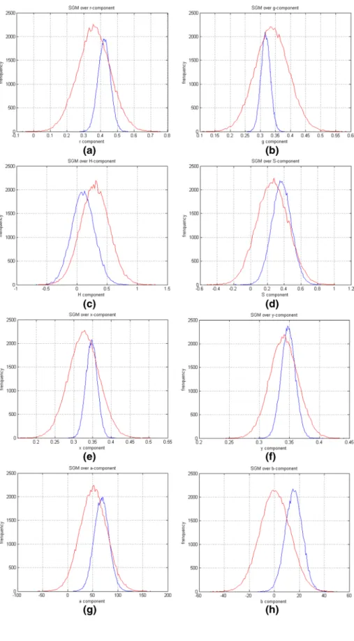
Figure 1 illustrates the SGM model applied to different colour spaces (nRGB, HSV, CIE X, Y, Z, and CIE L*, a*,
Fig. 1 The blue line represents skin and the red line represents background SGM. a Estimated SGM for r-component of nRGB. b Estimated SGM for g-com-ponent of nRGB. c Estimated SGM for H-component of HSV. d Estimated SGM for S-compo-nent of HSV. e Estimated SGM for x-component of CIE X, Y, Z. f Estimated SGM for y-compo-nent of CIE X, Y, Z. g Estimated SGM for a-component of CIE
L*, a*, b*. h Estimated SGM for b-component of CIE L*, a*,
b*). It is evident that the SGM model covers the entire area of the distribution for both skin and background. In some col-our spaces, the differentiation is greater, but the overlapping between skin and non-skin regions is sufficient to produce high false positive rate (FPR). As such, an SGM distribution can-not model all possible variation in the skin colour data. The existing approaches [6, 50] were extended by using Gaussian Mixture Models [36, 53].
2.1.2 Probabilistic colour models: Gaussian mixture model
Below we summarise the steps involved in a MG skin colour model.
• Firstly, the variance caused by the intensity is removed. This is achieved by normalising the data or by transforming the original pixel values into a different colour space (e.g., rg colour space [38] or HSV colour space [35]).
• Secondly, a colour histogram is computed, which is used to estimate an initial mixture model.
• Finally, a Gaussian mixture model is estimated, which can efficiently be done by applying the iterative EM-algorithm [10].
Assume a Gaussian mixture model:
where 𝜋(j) denotes the prior probability of expert j, and 𝜑(j) = {𝜇(j),𝛴(j)} denotes the parameters mean 𝜇(j) , and full-rank covariance matrix 𝛴(j) of the expert. The GMM’s output is given by:
where
is the jth Gaussian density of the GMM. The method for determining the parameters of a Gaussian mixture model from a data set is based on maximising the data likelihood.
Because the likelihood is a differentiable function, it is pos-sible to use general purpose optimisation algorithms such as the EM algorithm for fast convergence. After the initialisa-tion of 𝜃0 , the EM iteration is as follows:
(5) 𝜃={𝜋(j),𝜑(j) = {𝜇(j),𝛴(j)}; j=1,… …, J} (6) p(xt|𝜃) = J ∑ j=1 𝜋(j)p ( xt|𝛿t(j) =1,𝜑(j) ) (7) p ( xt|𝛿t(j) =1,𝜑(j) ) = (2𝜋)−D2|𝛴(j)|− 1 2 exp { −1 2(xt− 𝜇 (j))T(𝛴(j))−1(x t− 𝜇(j)) } (8) L(X|𝜃n)≡log p(X|𝜃n) =∑ Z P(Z|X,𝜃n)log p(X|𝜃n)
1. E-step As we do not know the class labels, but do know their probability distribution, what we can do is to use the expected values of the class labels given the current parameters. For the nth iteration, we form the function Q(𝜃|𝜃n) as follows:
and define
Using Bayes’ theorem, we can calculate h(nj)(xt) as:
which is actually the expected posterior distribution of the class labels given the observed data. In other words, the probability that xt belongs to group j given the
cur-rent estimates 𝜃n is given by h (j)
n(xt) . The calculation of
Q is the E-step of the algorithm and determines the best guess of the membership function h(nj)(xt).
2. To compute the new set of parameter values of
𝜃 (denoted as 𝜃∗ ), we optimise Q(𝜃|𝜃n) ; such as
𝜃∗ =arg max
𝜃Q(𝜃|𝜃n). This is the M-step of the algo-rithm.
Specifically, the steps are:
• Maximise Q(𝜃|𝜃n) with respect to 𝜃 to find 𝜃∗.
• Replace 𝜃n by 𝜃∗.
• Increment n by 1 and repeat the E-step until con-vergence.
To determine 𝜇(k)∗ , differentiate Q with respect to 𝜇(k) and equate to zero (𝜗Q(𝜃|𝜃n)
𝜗𝜇(k) =0) which gives:
To determine 𝛴(k)∗ , differentiate Q with respect to 𝛴(k) and equate to zero (𝜗Q(𝜃|𝜃n)
𝜗𝛴(k) =0) which gives:
To determine 𝜋(k)∗ , maximise Q(𝜃|𝜃n) with respect to 𝜋(k) subject to the constraint 𝛴J
j=1𝜋 j=1 which gives: (9) Q(𝜃|𝜃n) =E{log p(Z, X|𝜃)|X,𝜃n} = T ∑ t=1 J ∑ j=1 E{𝛿t(j)|xt,𝜃n}log [ p(xt|𝛿t(j)=1,𝜑(j))𝜋(j) ] (10) h(nj)(xt)≡E { 𝛿t(j)|xt,𝜃n } =P ( 𝛿(tj)=1|xt,𝜃n ) (11) h(nj)(xt) = p � xt�𝛿(tj)=1,𝜑(nj) � 𝜋n(j) ∑J k=1p � xt�𝛿 (k) t =1,𝜑 (k) n � 𝜋(nk) (12) 𝜇(k)∗= ∑T t=1h k n(xt)xt ∑T t=1hkn(xt) (13) 𝛴(k)∗ = ∑T t=1h k n(xt)(xt− 𝜇(k)∗)(xt− 𝜇(k)∗)T ∑T t=1hkn(xt)
(14) 𝜋(k)∗ = 1 T T ∑ t=1 hkn(xt)
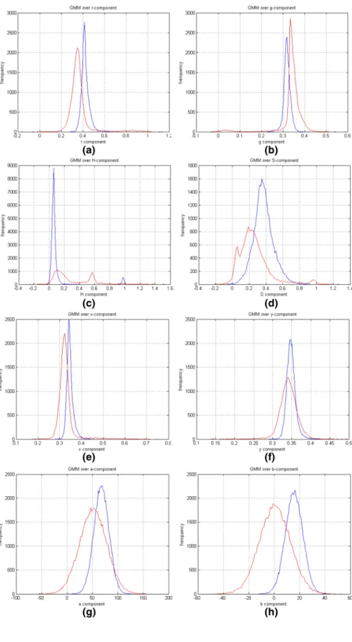
The two steps are repeated until the likelihood does not change significantly or the maximum number of iterations is reached. The GMMs obtained after 5 EM iterations for
Fig. 2 The blue line represents skin and the red line represents background GMM. a Estimated GMM for r-component of nRGB. b Estimated GMM for g-component of nRGB. c Esti-mated GMM for H-component of HSV. d Estimated GMM for S-component of HSV. e Esti-mated GMM for x-component of CIE X, Y, Z. f Estimated GMM for y-component of CIE
X, Y, Z. g Estimated GMM for a-component of CIE L*,
a*, b*. h Estimated GMM for b-component of CIE L*, a*, b* (colour figure online)
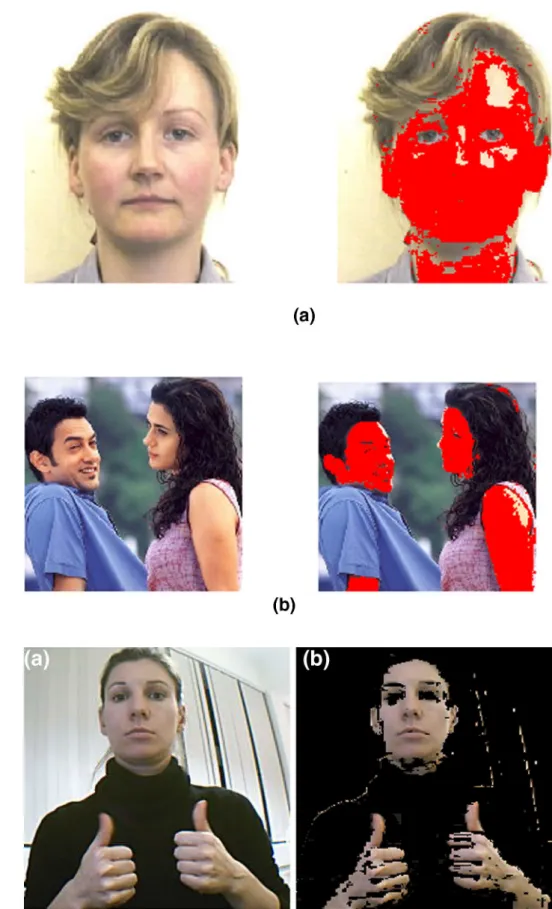
Fig. 3 a, b Image segmentation on simple background based on skin colour information. Skin area marked in red (colour figure online)
Fig. 4 Image segmentation on a different background based on skin colour information. a original input image, and b probability map for the skin colour
the different colour spaces (nRGB, HSV, CIE X, Y, Z, and CIE L*, a*, b*) are shown in Fig. 2.
The results were obtained from a database containing approximately one half million pixels.
Figures 3 and 4 show the GMM probability map for CIE L*, a*, b* skin colour against different backgrounds,
which can then be used to initialise the network for the GNG algorithm.
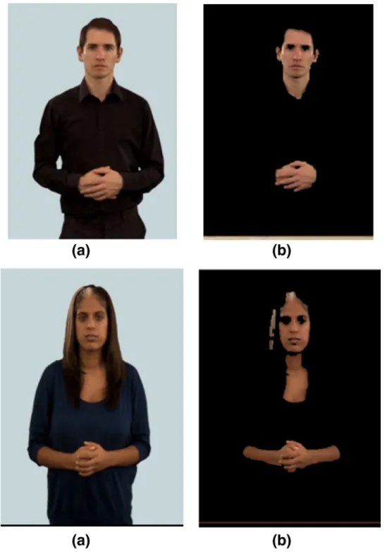
Figure 5 shows another example of the probability map for skin colour in deaf individuals, using normal 2D
Fig. 5 Image segmentation by skin colour in the BSL Sign-bank dataset. a Original input image, and b probability map for the skin colour
videos freely available from the BSL SignBank dataset,5
which can then be implemented with the specific goal of developing an automated dementia screening toolkit. In all three examples, the colour space used to represent the input image plays an important part in the segmentation. As we have seen above, some models are more perceptu-ally uniform than others and some separate out informa-tion such as luminance and chrominance.
At each node of the network, we experimented with more cluttered backgrounds with the perceptually uniform colour model CIE L*, a*, b*, and the non-perceptually uniform col-our models, nRGB, and CIE X, Y, Z. We also experimented
with the HSV colour model, which separates the bright-ness component from hue and saturation, to compensate for changes in illumination (Fig. 6). Unlike CIE L*, a*, b*, HSV is not perceptually mapped to the human visual sys-tem, meaning changes in colour values are not proportional to changes in the perceived significance of the change. A detailed discussion of the different colour models can be found in [23, 43, 48].
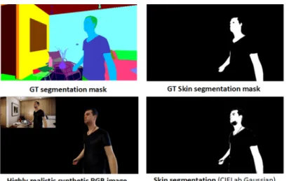
In order to address some of the challenges we face in real environments with changes in illumination, shadows and more cluttered backgrounds, we have tested the different chrominance models on two synthetic images we have gener-ated with our virtual environment UnrealROX [32]. Figure 7 shows the segmentation of the skin colour after applying the four different chrominance models and getting the skin
Fig. 6 Skin colour images in cluttered backgrounds. Top row shows the original images followed by the various colour spaces
probability with a GMM. Qualitative results demonstrate CIE L*, a*, b*, as the most efficient for skin segmentation since it is the most perceptually mapped to the visual system.
Given consideration of perceptual uniformity our best option is the CIE L*, a*, b* colour space. Thus, we converted the RGB values to the CIE L*, a*, b* values. The colour con-version from RGB to CIE L*, a*, b* is obtained by undergoing
a linear conversion from RGB to CIE X, Y, Z, and a nonlinear conversion from CIE X, Y, Z to CIE L*, a*, b*.
(15) ⎡ ⎢ ⎢ ⎣ X Y Z ⎤ ⎥ ⎥ ⎦ = ⎡ ⎢ ⎢ ⎣ 0.433910 0.376220 0.189860 0.212649 0.715169 0.072182 0.017756 0.109478 0.872915 ⎤ ⎥ ⎥ ⎦ ∗ ⎡ ⎢ ⎢ ⎣ R G B ⎤ ⎥ ⎥ ⎦
Fig. 7 Image segmentation on two synthetic images generated with UnrealROX [32]. From top to bottom, original input image, and probability maps for the skin colour after applying the four different chrominance models
where (16) L∗=116∗f [Y Yn ] −16 a∗ =500∗[f[X Xn ] −f [Y Yn ]] b∗ =200∗[f [Y Yn ] −f [Z Zn ]] (17) f(r) = { r13 if r>0.008856 7.7867∗r+ 16 116 if r≤0.008856 }
The Xn , Yn and Zn refer to the CIE X, Y, Z values for a speci-fied white point. To get the learning process started, we need a simple but robust method to obtain the topology preserv-ing graph (TPG) with as little user intervention as possible. Henceforth, the topology preserving graph TPG=⟨N, C⟩ is defined with a vertex (neurons) set N and an edge set C that connects them. The self-organising neural network growing neural gas (GNG) is used to filter out non-face candidates and detect and reconstruct the face and or the hands.
3 Growing neural gas (GNG) algorithm in 2D
and 3D
In order to determine where to insert new neurons, local error measures are gathered during the adaptation process and each new unit is inserted near the neuron which has the highest accumulated error. At each adaptation step, a connection between the winner and the second-nearest neuron is created as dictated by the competitive Hebbian learning algorithm. This is continued until an ending con-dition is fulfilled, as for example evaluation of the opti-mal network topology based on the topographic product [16]. This measure is used to detect deviations between the dimensionalities of the network and that of the input space, detecting folds in the network and indications that it is trying to approximate to an input manifold with differ-ent dimensions. In addition, in a GNG network the learn-ing parameters are constant in time, in contrast to other methods where learning is based on decaying parameters.
The network is specified as:
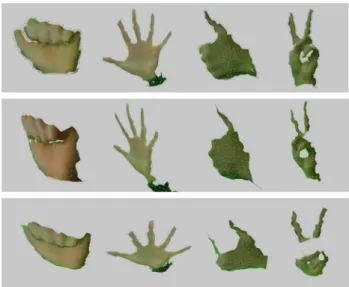
Fig. 8 GNG 3D surface reconstructions. 3D reconstruction of differ-ent hand poses obtained using the Kinect sensor
Fig. 9 Overview of the whole process using the first synthetic sam-ple. Top row shows the ground truth segmentation and skin masks. Bottom part shows skin segmentation results using CIE L*, a*, b*
(Gaussian). The images on the right show the error map of the com-puted skin mask and the 3D reconstructed mesh using the GNG algo-rithm
• A set N of nodes (neurons). Each neuron c∈N has
its associated reference vector wc∈Rd . The reference vectors can be regarded as positions in the input space of their corresponding neurons.
• A set of edges (connections) between pairs of neurons. These connections are not weighted and their purpose is to define the topological structure. The edges are determined using the competitive Hebbian learning algorithm. An edge ageing scheme is used to remove connections that are invalid because of the activation of the neuron during the adaptation process.
Fig. 10 Overview of the whole process using the second synthetic sample. Top row shows the ground truth segmentation and skin masks. Bottom part shows skin segmentation results using CIE L*,
a*, b* (Gaussian). The images on the right show the error map of the computed skin mask and the 3D reconstructed mesh using the GNG algorithm
The GNG learning is presented in Algorithm 1. With the new advances of low-cost 3D sensors, it is possible to gen-erate more natural gesture-based 3D interactions. However, these systems need to address the problem of 3D tracking of hand joints. In [2], the original GNG algorithm is extended to perform 3D surface reconstruction by considering surface normal information during the learning process. It also mod-ifies the original competitive Hebbian learning process by producing wire-frame 3D representations. In order to obtain 3D information in the form of point clouds, we had to project
disparity information obtained from the device to the three-dimensional space using the known geometry of the sensor. The relationship between a disparity map provided by the Kinect sensor and a normalised disparity map is given by d=1∕8⋅(doff−kd) , where d is the normalised disparity, kd is the disparity provided by the Kinect and doff is a particular
offset of a Kinect sensor. Calibration values can be obtained in the calibration step [25]. Figure 8 shows the 3D mesh cre-ated using the method discussed in [2].
It can be seen how this extended algorithm is able to cre-ate a coloured 3D mesh that represents the input data. Since point clouds obtained using the Kinect are partial 3D views, the mesh obtained is not complete and therefore the model generated by the GNG is an open coloured mesh.
Figures 9 and 10 show the whole process for different input samples that were synthetically generated using Unre-alROX [32]. From left to right, we can see the original RGB image and its corresponding ground truth segmentation mask. The ground truth segmentation mask for the skin class and the obtained results using the proposed method (CIE L*, a*, b* Gaussian). Finally, on the right we can see the 3D reconstruction results using as an input the skin mask, RGB and depth images. Using the GNG algorithm we are able to create a simplified coloured mesh from the input data. Since the skin mask has some false positives, the reconstructed mesh also shows small outliers.
4 Experiments
In this section, different experiments are shown validating the capabilities of our method (e.g. which statistical model is best for GNG reconstruction) which has also been used in 3D datasets. We tested our system on our own data set (University of Alicante, and University of Westminster) of faces and hands recorded from 15 participants. To create this data set we have recorded images over several days using a simple webcam with image resolution 800×600 . In total, we have recorded over 112,500 frames, and for computa-tional efficiency, we have resized the images to 300×225 ,
200×160 , 198×234 , and 124×123 pixels. In addition, experiments were conducted based on two publicly available
Table 1 IoU and Dice score for synthetic image 1
Bold indicates the best achieved score
Scene Frame Algorithm Dice score IoU score
1 1 CIELabsinglegaussian 0.874067744 0.776282803
1 1 CIELabmultigaussian 0.860429045 0.755023416
1 1 CIExyzsinglegaussian 0.729085392 0.573655639 1 1 CIExyzmultigaussian 0.763614975 0.617600418
1 1 HSVsinglegaussian 0.74712024 0.596304817
1 1 HSVmultigaussian 0.760118655 0.613039857
1 1 nRGBsinglegaussian 0.773454371 0.630579375
1 1 nRGBmultigaussian 0.766449414 0.621317352
databases, Mikkel B. Stegmann6 and Stirling’s.7 All methods
have been developed and tested on a desktop machine of 2.26 GHz Pentium IV processor. These methods have been implemented in MATLAB and C++.
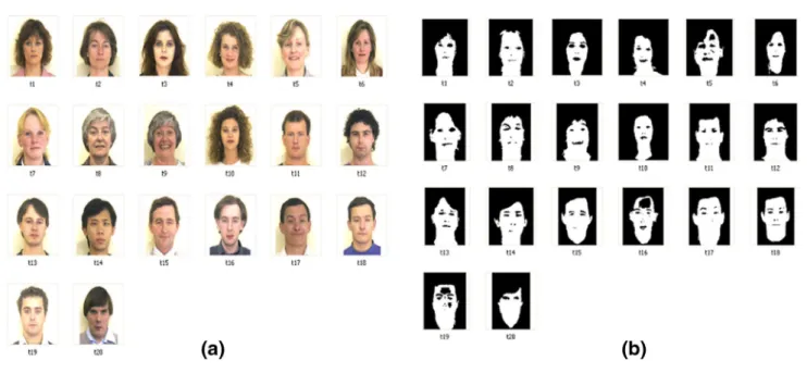
Figure 11 shows the ground truth model which we use to measure the error produced by our method. To measure the class probability of skin to non-skin regions we use the positive (TPR) and false positive (FPR) rates as obtained by:
where TP is number of true positive (pixels correctly assigned to the skin class). FP is the number of false posi-tives (non-skin pixels wrongly assigned to skin). S is the total of skin pixels and NS the totals of non-skin pixels. These rates TPR and FPR are calculated using both models (SGM and GMM) for all test images. Through this computa-tion we get vector of measures P= (TPR, FPR) that express
performance of the given model. In order to measure the similarity between the predicted skin colour region and the ground truth region in the two synthetic images, we applied the Intersection over Union (IoU) metric, as a standard per-formance measure for all the four chrominance models. The IoU metric measures the number of pixels common to both the target and prediction regions, divided by the total num-ber of pixels present across both regions.
We also calculated the loss function of our image segmen-tation tasks in the two synthetic images based on the Dice coefficient calculated as:
Tables 1 and 2 show the results.
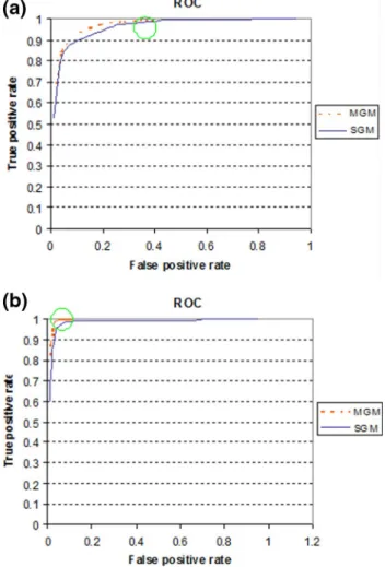
For further comparison between the SGM and the GMM model, we used ROC curves for all the test images. For drawing ROC curves, we calculated TPR and FPR for all images using different threshold (threshold value is set as per P(S|x)� ). Thus by using K different thresholds, we can get K point vectors, which, when plotted, results in a ROC curve for the specific model with respect to test image.
Figure 12, shows ROC curves for the test images 4 and 17, respectively, from Fig. 11. It is clear from the ROC curve that both SGM and GMM have almost the same TPR. The FPR in GMM curve (orange dotted line) becomes constant at a certain threshold, as shown by the green circle. However, FPR for SGM (blue line) keeps increasing as the threshold value decreases. FPR reaches nearly to 0.9. Several of the thresholds for images 4 and 17 are shown in Figs. 13 and 14 respectively. From the threshold images, it is very clear that SGM images have a higher FPR rate. Based on the ROC (18) TPR= TP S (19) FPR= FP NS (20)
IoU= target∩prediction target∪prediction
(21)
Dice= 2∣target∩prediction∣ ∣target∣ + ∣prediction∣
Table 2 IoU and Dice score for synthetic image 2
Bold indicates the best achieved score
Scene Frame Algorithm Dice score IoU score
1 2 CIELabsinglegaussian 0.898387257 0.815509983
1 2 CIELabmultigaussian 0.935972544 0.879640743
1 2 CIExyzsinglegaussian 0.74361557 0.591862691
1 2 CIExyzmultigaussian 0.910774728 0.836158347
1 2 HSVsinglegaussian 0.930137277 0.86938926
1 2 HSVmultigaussian 0.882018032 0.788929152
1 2 nRGBsinglegaussian 0.901852199 0.821238972
1 2 nRGBmultigaussian 0.891526587 0.804274396
Fig. 12 a ROC curve for test image 4. b ROC curve for test image 17
7 http://pics.psych .stir.ac.uk/. 6 http://www2.imm.dtu.dk/~aam/.
Fig. 13 Image 4 threshold representation for GMM (1 row) and SGM (2 row). Threshold values for each column are 0.7, 0.6, 0.5, and 0.4 respectively
Fig. 14 Image 17 threshold representation for GMM (1 row) and SGM (2 row). Threshold values for each column are 0.7, 0.6, 0.5, and 0.4 respectively
Table 3 TPR and FPR rates for all four colour spaces using SGM
Bold indicates the best achieved score
HSV CIE X, Y, Z nRGB CIE L*, a*, b* TPR FPR TPR FPR TPR FPR TPR FPR 0.5689 0.2395 0.8442 0.1341 0.9156 0.207 0.8902 0.1031 0.8947 0.0995 0.9371 0.0596 0.9641 0.1183 0.9471 0.0485 0.7538 0.2632 0.8655 0.1985 0.9708 0.2683 0.8015 0.1583 0.8568 0.2706 0.8915 0.0969 0.9198 0.1581 0.9015 0.0889 0.6378 0.161 0.9019 0.0709 0.9492 0.1263 0.9159 0.0719 0.9337 0.2527 0.8587 0.1117 0.9217 0.1669 0.9587 0.1011 0.6664 0.1598 0.8383 0.0628 0.8966 0.0813 0.8983 0.0528 0.8742 0.0529 0.9247 0.0822 0.9544 0.1352 0.9201 0.0501 0.9083 0.109 0.8353 0.0341 0.8943 0.0548 0.8853 0.0508 0.512 0.297 0.7843 0.1163 0.8836 0.1787 0.8513 0.0963 0.7496 0.0788 0.9172 0.0607 0.9527 0.1021 0.9561 0.0531 0.7915 0.0395 0.969 0.0506 0.9834 0.0757 0.9598 0.0306 0.8437 0.0789 0.8005 0.0535 0.8713 0.0806 0.8995 0.0555 0.65 0.0373 0.7279 0.0401 0.8249 0.0594 0.8271 0.0324 0.8503 0.0931 0.9284 0.0864 0.9606 0.1403 0.9684 0.0804 0.2353 0.1242 0.7993 0.0483 0.9435 0.0254 0.7803 0.0382 0.9598 0.0362 0.9364 0.0349 0.9641 0.054 0.9164 0.0312 0.8857 0.0255 0.9501 0.0383 0.9753 0.0556 0.9511 0.0213 0.5688 0.0254 0.8118 0.0471 0.9114 0.0984 0.9108 0.0206 0.7346 0.0315 0.8503 0.0214 0.9173 0.0409 0.9403 0.0184
Table 4 TPR and FPR rates for all four colour spaces using GMM
Bold indicates the best achieved score
HSV CIE X, Y, Z nRGB CIE L*, a*, b* TPR FPR TPR FPR TPR FPR TPR FPR 0.9228 0.2374 0.8518 0.2256 0.7931 0.2654 0.8831 0.2211 0.9516 0.0654 0.9699 0.0837 0.9638 0.0832 0.9238 0.0499 0.8128 0.3118 0.9151 0.2794 0.9063 0.3241 0.8813 0.2683 0.9726 0.165 0.9685 0.1486 0.9454 0.1939 0.9754 0.0912 0.9009 0.1065 0.9357 0.0921 0.9388 0.1135 0.8988 0.0989 0.9895 0.1777 0.994 0.1649 0.992 0.2053 0.9882 0.1541 0.989 0.1263 0.985 0.1273 0.9745 0.0949 0.9275 0.0928 0.9644 0.0878 0.9728 0.0995 0.9637 0.1042 0.9644 0.0801 0.9662 0.0579 0.9699 0.0646 0.9647 0.0705 0.9641 0.0508 0.9793 0.2022 0.7551 0.1755 0.7528 0.23 0.8328 0.0963 0.9938 0.0639 0.9395 0.0785 0.9359 0.076 0.9959 0.0531 0.9857 0.0628 0.9906 0.0643 0.9874 0.0693 0.9751 0.0306 0.9001 0.0627 0.9335 0.0708 0.8903 0.0694 0.9003 0.0535 0.9714 0.0445 0.8289 0.0501 0.8141 0.0494 0.9541 0.0324 0.9936 0.0897 0.9985 0.1050 0.9952 0.1078 0.9952 0.0804 0.9578 0.0753 0.9596 0.0703 0.9691 0.0894 0.9990 0.0382 0.9911 0.0363 0.9925 0.0409 0.9893 0.0429 0.9589 0.0312 0.9888 0.0438 0.9948 0.0495 0.9894 0.0462 0.9899 0.0213 0.7673 0.0446 0.8534 0.0525 0.8515 0.0574 0.8001 0.0206 0.9329 0.0267 0.9448 0.0243 0.9451 0.0283 0.9479 0.0184
curves for all test images, it is evident that SGM have a very high FPR and thus they perform badly as compared to GMM. Additionally, for several images TPR at a given threshold for SGM was marginally low as compared to GMM. This mar-ginally low TPR will not have any effect on the images with large skin area. Nevertheless for the images with small skin area (small faces), this low TPR can have an adverse effect.
Tables 3 and 4 show calculated TPR and FPR for all four colour spaces using the SGM and GMM statistical models, respectively. For the calculations, we have used a fixed threshold value of 0.55, since it is the middle range value where we can find the highest TPR and lowest FPR for comparison purposes. It can be seen how the CIE L*, a*, b* model outperforms all other three colour spaces since it has the lowest FPR rate among the 20 images, fol-lowed by the CIE X, Y, Z. The comparisons demonstrate that GMM outperforms SGM with low FPR rate, which makes it a suitable model for image segmentation espe-cially in cases where hands and faces are involved. This is then used in the initialisation of the first frame of the GNG algorithm.
Figure 15 shows the correctly detected hands and face after applying EM to segment the skin region. The recon-struction of the 2D topology of both hands and face is done with the GNG algorithm.Figure 16 shows the 3D reconstruction of a human face acquired using the Kinect sensor (top) and the 3D reconstruction of a synthetically generated human face (bottom). Both faces were recon-structed using the GNG for 3D surface reconstruction discussed in Sect. 4. Synthetic data was generated using Blensor software [18], for simulating a virtual Kinect sen-sor (noise-free).
While 3D downsampling and reconstruction methods like Poisson or Voxelgrid are not able to deal with noisy data, the GNG method is able to avoid outliers and obtain an accurate representation in the presence of noise. This ability is due to the Hebbian learning rule used and its random nature that updates vertex locations based on the average influence of a large number of input patterns.
Fig. 15 a Original image, b after applying EM to segment skin region, and c hand and face 2D topology with the GNG network
Fig. 16 GNG 3D reconstructions. Top: 3D face reconstruction from data obtained using the Kinect sensor. Bottom: 3D face reconstruc-tion from data synthetically generated using Blensor software
5 Conclusions and future work
In this paper, we have compared the performance of dif-ferent probabilistic colour models and colour spaces for skin segmentation as an initialisation stage for the GNG algorithm. Based on the capabilities of GNG to readjust to new input patterns without restarting the learning process, we are interested in reducing meaningless image data by taking into consideration that human skin has a relatively unique colour and applying appropriate parametric skin distribution modelling. We concluded that GMM was superior to SGM with lower FPR rates. We also showed that CIE L*, a*, b* colour space outperforms all three other colour spaces since it has the lowest FPR rate among the dataset. **Preprocessing was also used as an initiali-sation stage in the 3D reconstruction of faces and hands based on the work conducted in [2]. Further work will aim at improving system performance by accelerating GPUs which can then be used for robotic system recognition. Nonetheless, we are currently working, after obtaining a clean segmentation, on hand sign trajectories in order to analyse the sign space envelope (sign trajectories/depth/ speed) and facial expressions of deaf individuals. An automated screening toolkit will be beneficial not only to screening of deaf individuals for dementia, but also for assessment of other acquired neurological impairments associated with motor changes, for example, stroke and Parkinson’s disease.
Funding This work has been supported by the Spanish Government
TIN2016-76515R Grant, supported with FEDER funds, the Univer-sity of Alicante Project GRE16-19, the Valencian Government Project GV-2018-022, and the UK Dunhill Medical Trust Grant RPGF1802\37. Open Access This article is distributed under the terms of the Crea-tive Commons Attribution 4.0 International License (http://creat iveco mmons .org/licen ses/by/4.0/), which permits unrestricted use, distribu-tion, and reproduction in any medium, provided you give appropriate credit to the original author(s) and the source, provide a link to the Creative Commons license, and indicate if changes were made.
References
1. Albrecht I, J Haber, H Seidel (2003) Construction and animation of anatomically based human hand models. In: Proceedings of the 2003 ACM SIGGRAPH/Eurographics symposium on computer animation, pp 98–109
2. Angelopoulou A, Garcia-Rodriguez J, Orts Escolano S, Gupta G, Psarrou A (2018) Fast 2d/3d object representation with growing neural gas. Neural Comput Appl 29(10):903–919
3. Athency A, Ancy BM, Fathima K, Dilin R, Binish M (2017) Brain tumor detection and classification in MRI images. Int J Innov Res Sci Eng Technol 6:84–89
4. Boehme H, Brakensiek A, Braumann U, Krabbes M, Gross H (1998) Neural networks for gesture-based remote control of a mobile robot. Proc IEEE World Congr Comput Intell 1:372–377 5. Cédras C, Shah M (1995) Motion-based recognition: a survey.
Image Vis Comput 13(2):129–155
6. Caetano S, Olabarriaga S, Barone AC (2002) Performance evalu-ation of single and multiple-Gaussian models for skin color mod-eling. In: Proceedings of the Brazilian symposium on computer graphics and image processing-SIBGRAPI, pp 275–282 7. Cheng H, Jiang X, Sun Y, Wang J (2001) Color image
segmenta-tion: advances and prospects. Pattern Recognit 34(12):2259–2281 8. Cretu, A, Petriu E, Payeur P (2008) Evaluation of growing neural
gas networks for selective 3D scanning. In: Proceedings of IEEE international workshop on robotics and sensors environments, pp 108–113
9. De la Torre F, Black M (2001) Probabilistic principal component analysis. In: Proceedings of the IEEE international conference on computer vision, vol I, pp 362–369
10. Dempster A, Laird N, Rubin D (1977) Maximum likelihood from incomplete data via the em algorithm. J R Stat Soc B 39(1):1–38 11. Eddy S (1996) Hidden Markov models. Curr Opin Struct Biol
6(3):361–365
12. Friedman N, Russel S (1997) Image segmentation in video sequences: a probabilistic approach. In: Proceedings of the con-ference on uncertainty in artificial intelligence, pp 175–181 13. Fritzke B (1994) Growing cell structures—a self-organising
net-work for unsupervised and supervised learning. J Neural Netw 7(9):1441–1460
14. Fritzke B (1995) A growing neural gas network learns topolo-gies. In: Advances in neural information processing systems 7 (NIPS’94), pp 625–632
15. García-Rodríguez J, Angelopoulou A, Psarrou A (2006) Growing neural gas (GNG): a soft competitive learning method for 2D hand modeling. IEICE Trans Inf Syst E89–D(7):2124–2131
16. Geoffrey J, Goodhill F, Terrence J (1997) A unifying measure for neighbourhood preservation in topographic mappings. In: Pro-ceedings of the 2nd joint symposium on neural computation, vol 5, pp 191–202
17. Ghazali KHB, Ma J, Xiao R, lubis SA (2012) An innovative face detection based on YCgCr color space. Phys Procedia 25(0):2116–2124
18. Gschwandtner M, Kwitt R, Uhl A, Pree W (2011) BlenSor: blender sensor simulation toolbox advances in visual computing. volume 6939 of lecture notes in computer science, chapter 20. Springer, Berlin, pp 199–208
19. Gupta G, Psarrou A, Angelopoulou A, García J (2012) Region analysis through close contour transformation using growing neu-ral gas. In: Proceedings of the international joint conference on neural networks, IJCNN2012, pp 1–8
20. Holdstein Y, Fischer A (2008) Three-dimensional surface recon-struction using meshing growing neural gas ( MGNG). Vis Com-put Int J ComCom-put Graph 24(4):295–302
21. Hye-Rin K, Seon J K, In-Kwon L (2017) Building emotional machines: recognizing image emotions through deep neural net-works. CoRR arXiv :abs/1705.07543
22. Jones M, Rehg J (2002) Statistical color models with application to skin detection. Int J Comput Vis 46(1):81–96
23. Kakumanu P, Makrogiannis S, Bourbakis N (2007) A survey of skin-color modeling and detection methods. Pattern Recognit 40(3):1106–1122
24. Khan R, Hanbury A, Stttinger J, Bais A (2012) Color based skin classification. Pattern Recognit Lett 33(2):157–163
25. Khoshelham K, Elberink SO (2012) Accuracy and resolution of Kinect depth data for indoor mapping applications. Sensors 12(2):1437–1454
26. Koike H, Sato Y, Kobayashi Y (2001) Integrating paper and digital information on enhanced desk: a method for real time finger tracking on an augmented desk system. ACM Trans Com-put Hum Interact 8(4):307–322
27. Kolkur, S, Kalbande D, Shimpi P, Bapat C, Jatakia J (2017) Human skin detection using RGB, HSV and YCbCr color mod-els. CoRR arXiv :abs/1708.02694
28. Lee M, Nevatia R (2005) Integrating component cues for human pose estimation. In: Proceedings of the IEEE international workshop on visual surveillance and performance evaluation of tracking and surveillance, pp 41–48
29. Lucchese L, Mitra S (2001) Color image segmentation: a state-of-the-art survey. Proc Indian Natl Sci Acad (INSA-A) 67(2):207–221
30. Martinez T (1993) Competitive Hebbian learning rule forms perfectly topology preserving maps. In: ICANN93: international conference on artificial neural networks, pp 427–434
31. Martinetz TM, Schulten KJ (1991) A "neural-gas" network learns topologies. In: Kohonen T, Makisara K, Simula 0, Kan-gas J (eds) Artificial Neural Networks, pp 397–402. North-Holland, Amsterdam
32. Martinez-Gonzalez P, Oprea S, Garcia-Garcia A, Jover-Alva-rez A, Orts-Escolano S, Rodríguez JG (2018) Unrealrox: an extremely photorealistic virtual reality environment for robot-ics simulations and synthetic data generation. CoRR arXiv :abs/1810.06936
33. Nair V, Clark J (2004) An unsupervised, online learning frame-work for moving object detection. In: Proceedings of the IEEE conference on computer vision and pattern recongition, vol II, pp 317–324
34. Oliver N, Rosario B, Pentland A (2000) A Bayesian computer vision system for modelling human interactions. IEEE Trans Pat-tern Anal Mach Intell 22(8):831–843
35. Raja Y, McKenna S, Gong S (1998) Colour model selection and adaptation in dynamic scenes. In: Proceedings of the European conference on computer vision, pp 460–474
36. Redner R, Walker H (1984) Mixture densities, maximum likeli-hood and the EM algorithm. SIAM Rev 26(2):195–239 37. Rêgo R, Araújo A, de Lima Neto F (2007) Growing
self-organ-izing maps for surface reconstruction from unstructured point clouds. In: Proceedings of the international joint conference on artificial neural networks, IJCNN’07, pp 1900–1905
38. Schwerdt K, Crowley J (2000) Robust face tracking using color. In: Proceedings of the international conference on automatic face and gesture recognition, pp 90–95
39. Sharifara A, Rahim MSM, Navabifar F, Ebert D, Ghaderi A, Papa-kostas M (2017) Enhanced facial recognition framework based on skin tone and false alarm rejection. In: Proceedings of the 10th international conference on PErvasive technologies related to assistive environments, PETRA ’17. ACM, pp 240–241 40. Sivic J, Everingham M, Zisserman A (2005) Person spotting:
video shot retrieval for face sets. In: International conference on image and video retrieval, pp 226–236
41. Sonka M, Hlavac V, Boyle R (1998) Image processing, analysis, and machine vision. CL-Engineering, 2nd edn, pp 513–524 42. Stauffer C, Grimson W (1999) Adaptive background mixture
mod-els for real-time tracking. In: Proceedings of the IEEE conference on computer vision and pattern recognition, vol II, pp 246–252 43. Störring M (2004) Computer vision and human skin colour. Ph.D.
thesis, Aalborg University
44. Stergiopoulou E, Papamarkos N (2009) Hand gesture recognition using a neural network shape fitting technique. Eng Appl Artif Intell 22(8):1141–1158
45. Subasic M, Loncaric S, Birchbauer J (2009) Expert system segmentation of face images. Expert Syst Appl 36(3, Part 1):4497–4507
46. Sui C (2011) Appearance-based hand gesture identification. Uni-versity of New South Wales, Master of Engineering
47. Vamplew P, Adams A (1998) Recognition of sign language gestures using neural networks. Austr J Intell Inf Process Syst 5(2):94–102
48. Vezhnevets V, Sazonov V, Andreeva A (2000) A survey on pixel-based skin color detection techniques. In: Proceedings of the inter-national conference on automatic face and gesture recognition, pp 90–95
49. Wong S, Ranganath S (2005) Automatic sign language analysis: a survey and the future beyond lexical meaning. IEEE Trans Pattern Anal Mach Intell 6:873–891
50. Wren C, Azarbayejani A,D T, Pentland A (1997) Pfinder: real-time tracking of the human body. IEEE Trans Pattern Anal Mach Intell 19(7):780–785
51. Yan J, Zhang X, Lei Z, Li SZ (2014) Face detection by structural models. Image Vis Comput 32(10):790–799
52. Yang J, Bang W, Choi E, Cho S, Oh J, Cho J, Kim S, Ki E, Kim D (2009) A 3D hand-drawn gesture input device using fuzzy ARTMAP-based recognizer. J Syst Cybern Inform 4(3):1–7 53. Yang M, Ahuja N (1999) Gaussian mixture model for human skin
color and its applications in image and video databases. In: Pro-ceedings of SPIE99, pp 458–466
54. Zakaria Z, Suandi S A (2011) Combining skin color and cascade-like neural network for face detection. In: Proceedings of IEEE international conference on intelligent computing and intelligent systems, pp 587–591
55. Zariffa J, Steeves J (2011) Computer vision-based classification of hand grip variations in neurorehabilitation. In: Proceedings of 2011 IEEE international conference on rehabilitation robotics, pp 1–4
Publisher’s Note Springer Nature remains neutral with regard to

![Fig. 7 Image segmentation on two synthetic images generated with UnrealROX [32]. From top to bottom, original input image, and probability maps for the skin colour after applying the four different chrominance models](https://thumb-us.123doks.com/thumbv2/123dok_us/10989124.2986632/10.892.308.808.76.915/segmentation-synthetic-generated-unrealrox-original-probability-different-chrominance.webp)