Learning the Effectiveness of Content and Methodology in an Intelligent Tutoring System

(1)

Digital WPI

Masters Theses (All Theses, All Years)

Electronic Theses and Dissertations

2011-05-03

Learning the Effectiveness of Content and

Methodology in an Intelligent Tutoring System

Matthew D. Dailey

Worcester Polytechnic Institute

Follow this and additional works at:

https://digitalcommons.wpi.edu/etd-theses

This thesis is brought to you for free and open access byDigital WPI. It has been accepted for inclusion in Masters Theses (All Theses, All Years) by an authorized administrator of Digital WPI. For more information, please [email protected].

Repository Citation

Dailey, Matthew D., "Learning the Effectiveness of Content and Methodology in an Intelligent Tutoring System" (2011).Masters Theses (All Theses, All Years). 684.

(2)

by Matthew Dailey

A Thesis

Submitted to the Faculty of the

WORCESTER POLYTECHNIC INSTITUTE in partial fulfillment of the requirements for the

Degree of Master of Science in

Computer Science by

May 2011

APPROVED:

Professor Neil T. Heffernan, Major Advisor

Professor Gary Pollice, Thesis Reader

(3)

Classroom instruction time is a valuable yet scarce resource to teachers, who must decide how to best meet their objectives by selecting which topics to spend time on and when to move forward. Intelligent Tutoring Systems (ITS) are a powerful tool for teachers in this regard, allowing them to measure their students current level of knowledge, helping them gauge student knowledge ac-quisition, and providing them with valuable insight into learning methodologies. By using ITS to identify the effectiveness of proven methods of instruction, we can more effectively teach students both in and outside of the classroom. In this paper we review the results and contributions of a new Bayesian data mining method which can be used to identify what works in an ITS and how it can be used to learn from data which is not in the typical randomized controlled trial design. We then discuss modifications to this dataset which use more knowledge about the students to improve accuracy. Lastly we evaluate this model on detecting and predicting long term student retention, and discuss methods to improve its predictive accuracy.

(4)

Acknowledgements

I would like to thank the ASSISTments development team for their knowledge and support in this work. In particular I would like to thank Zachary Pardos for his research guidance my first year, and Zachary Broderick for his development assistance. I would also like to thank Neil and Cristina Heffernan for the opportunity to work on the ASSISTments project.

Funding for this research was provided primarily by the National Science Foundation’s GK-12 program, of which I am a fellow as part of the Partnership In Math and Science Education (PIMSE) grant. Additional sources of funding include the Department of Education, the Office of Naval Research, and the Spencer Foundation.

(5)

List of Figures

2.1 An example of two problems in ASSISTments that are from the same item template. An item template provides a skeleton form for a question, and allows large question banks to be created with low content development time. An item template can also make a skeleton form for tutoring. . . 6 2.2 A typical view of classes that a student is enrolled in. For the mastery learning

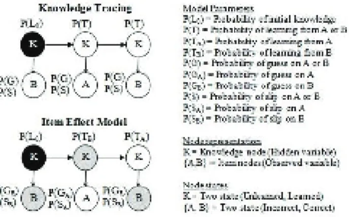
class, the student can take their reassessment test, or can complete one of their assignments, shown in red. The checkmarks next to an assignment name indicate the mastery level of the student. . . 8 3.1 An example of a three problem topology for Knowledge Tracing and the Item Effect

model including the associated parameters. The Item Effect Model learns additional parameters for each different item template in the problem set. . . 14 4.1 The Tutorial Effect Model with a sample set of student responses; correct, incorrect,

incorrect, correct (1,0,0,1). . . 20 5.1 The plotted matching guess and slip rates for the model with and without a correct

(7)

List of Tables

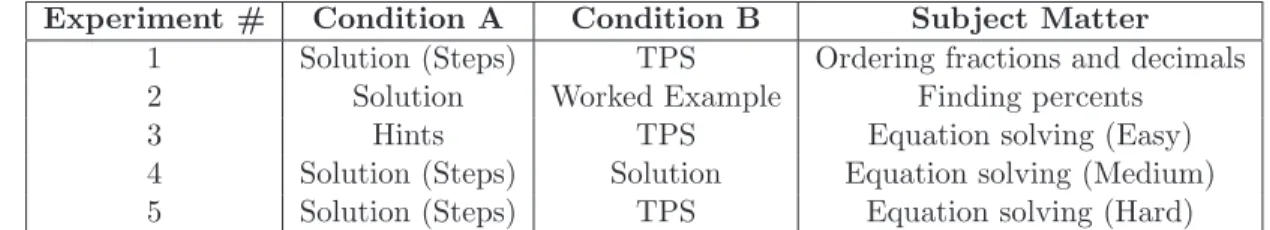
3.1 Five experiments were embedded into mastery learning problems sets. Each exper-iment compared the effectiveness of the tutorial feedback in Condition A with that in Condition B. . . 12 3.2 The results of comparing the Item Effect Model vs. t-tests to determine the

effec-tiveness of various methods of tutorial feedback within mastery assignments. . . 15 4.1 The statistics for five sample students are shown under the two bin splitting

pro-cedures. The last two columns show which knowledge class each student would be placed in for each of the splitting procedures. . . 24 4.2 Example of five students and using their statistic from Bin Split 1 to seed the prior

knowledge for the high knowledge class. . . 24 5.1 Comparison of cross fold validation results for the two bin splitting procedures with

prior set to average of first response. The last two rows state for the full prediction, how many times did each bin splitting procedure have the lower error rate. . . 28 5.2 The percentage correct for each of the five experiments by question. . . 28 5.3 Compares the actual percentage correct on each of the experimental problem sets to

the mean of the students system wide percentage correct. We can tell that experi-ments 2 through 5 are much harder than an average question. . . 29 5.4 Comparison of cross fold validation results for the two prior setting procedures when

bin split 1 is used. The last two rows state for the full prediction, how many times did each prior setting procedure have the lower error rate. . . 30 5.5 Comparison of cross fold validation results for the adapted Item Effect model with

and without a correct response explicitly modeled. . . 31 6.1 Shows the average error for three different metrics fo each of the starting seeds of

the forget value. Also shows the average prediction and percentage correct for each of these seeded forget rates . . . 36 6.2 Comparison of error metrics by same day and new day. . . 37

(8)

Chapter 1 Introduction

Today, Intelligent Tutoring Systems (ITS) arise not just in mathematical domains where they started, but also in physics, programming languages, speaking and reading, and even in scientific thought process. Their aim is to provide tutoring equivalent to, if not better than a human tutor, at a fraction of the price. [7] The tutoring system can provide a oneto-one interaction with students and address their individual needs, while not requiring the teacher to slow the entire class for one student. The student who needs additional help, is easily identified by the tutoring system, and given adjusted instruction. The teacher is then informed and can decide if additional steps can be taken.

Most student learning is done outside of the classroom where the teacher is not available. Web based tutoring can allow students to take the teacher wherever they go, including their home, a library or even on smart phones while riding the bus. The students have this highly interactive ap-paratus, which has been shown to increase learning when compared to paper and pencil homework. [9]

The creators of ITS attempt to provide the most beneficial content possible, as they want their product to be used. They are therefore very interested in developing cognitive models of student learning as well as determining information about their content. One area of research is identifying certain characteristics of knowledge components, which are very similar to mathematical skills. For example, the addition of two positive integers may be classified as easy to learn and easy to remember , while other skills are classified as slow to learn, but easy to remember. [16] One difficulty in this type of analysis is that the differences in the characteristic of knowledge components may

(9)

be very small. In the Reading Tutor from Project Listen, it is shown students learn to read very slowly, and therefore there was no difference in different types of tutoring It was later discovered this was due to the long time it takes a student to learn and the drastically slow learning rate. [10] The cognitive models which are created serve many purposes. They can be used to predict a students knowledge which is used to determine how many questions to give a student. If there is strong evidence a student knows the topic, the tutoring system will stop giving problems. This variable rate of problems goes against the ideas of mass practice and the one size fits all of set size nightly homework assignments. Additionally, the models can identify certain personas, or groups of students who benefit from one type of tutoring more than another. Students who are very smart and answer problems incorrectly because they have not seen them in the past, are very different from students who are in special needs. These models attempt to different classifications of students to allow for a more personalized tutoring experience.

There are millions of student responses generated by Intelligent Tutoring Systems annually, creating a rich source of data from which to learn what learning strategies and content are effective, and which ones are not. However, for most of this data, the format is not conducive to traditional educational research methods, and the data is not embedded between a pre and post test. As a result, much of this hard to analyze data is not analyzed, and from a research perspective, is wasted. We will present ways in which this data can be analyzed that will allow for these models to be developed and for pedagogical insights to be learned.

In [11], we discussed ways in which experimental designs can be found within log data even when the authors did not intend for the data to be from an experimental design. This was realized through demonstrations of how randomly assigned questions can form an experiment, since as data collects, it is as if students had been placed into conditions. However, since there was no posttest assessment given to the students, an evaluation method which could learn from the responses from students progressing through a set of problems was needed. By adapting known Bayesian methods to these domains, we showed posttest evaluations were not needed. This approach has practical effects such as being able to learn from teacher created content, which accounts for sixty four percent of the student responses within ASSISTments, a web based ITS.

Also in [11], we analyzed the Item Effect Model [12], a Bayesian network method which had been shown effective in simulated student data, but which had not been used on actual student data.

(10)

We used this method on eleven datasets from ASSISTments, and compared it to a more traditional t-test approach. We argued that even if the Bayesian method was not more powerful at detecting significant differences than the t-test, there was additional benefit in the other parameters of the Bayesian model. These included parameters for the relative difficulty and relative effectiveness of each of the problems. Through analyzing these datasets, we realized an early goal of a true embedded experiment in which students may be unaware of the condition in which they are placed. [1] We review some of these findings and then demonstrate how we can adapt our model to use more domain knowledge about students as well as how to model student learning more pedagogically correctly.

A critique of [11] led to a search of a retention rate for students that could be incorporated into the Item Effect Model. If the model detects differences in learning rates amongst types of help given to students, or amongst different formats knowledge components, do these necessarily translate into differences in long-term retention? We would like it, that if our model states there is a difference in learn rates among two types of help, that when students encounter a problem a week or a month later, those students who were exposed to the more beneficial help, can complete the related problem correctly a higher percentage of the time. At the time of [11], data of this format was not accessible. With a new system introduced into an Intelligent Tutoring System, we can both validate if our current model is able to predict long term student retention rates without modification, as well as discover the expected student retention rate for each knowledge component.

(11)

Chapter 2 Background

2.1 The ASSISTments System

The ASSISTments System [14] is a Web-based math and science tutor and assessment platform that allows teachers to easily find or create content to assign to their students.Students work through their assignments by answering multiple choice, fill-in, or even open response questions. These problems can give different types of tutorial feedback or tutoring to the students, which can either represent different pedagogical ways to solve the problem or different ways to present the material.Teachers can actively monitor how their students are progressing using reports that provide both question-by-question analyses as well as aggregated information.These reports are used to allow teachers to alter their plan and either review certain problem topics with students more, or bypass lessons where students are already knowledgeable. This process, known as formative assessment, plays a major role in the new federal Race to the Top initiative, in which teachers are encouraged to use student derived data to drive their classroom instruction. ASSISTments differs from other intelligent tutoring systems such as the Cognitive Tutor, the largest such ITS which started in Pittsburg, PA, since it gives teachers the control, and does not attempt to progress students through a curriculum. As a result, it is used as an addition to and not a replacement of classroom instruction.

ASSISTments mirrors a typical student school relationship. In ASSISTments, a student is enrolled in a school, and can join any class taught by one of the teachers at that school. The teacher can teach multiple classes and can even break a class down further if needed. This is often used

(12)

for teachers who teach, for example, multiple Algebra-2 classes. All students enroll in the teachers Algebra-2 class, and they are further broken down by what period they are in. Teachers can assign collections of problems known as a problem set to their students. When assigned to a class, we refer to these problem sets as assignments. These assignments can be homework assignments or could be intended to be solved in a computer lab.

On each of these assignments, students must complete problems until they meet some ending condition for the assignment. To help the students complete the problems, ASSISTments gives tutorial feedback or help to the students. This help takes many forms, and on each problem a student is randomly assigned to one of the possible types of help. The most common type of help in ASSISTments is hints, which are small instructions that provide progressively more of the solution to the problem. Often, the first hint provides a general reminder to the student of how to solve the problem. In ASSISTments, unlike some other ITS, when a student asks for help, he is marked incorrect on that problem.

The system is constantly being updated with new features that generate new and unique datasets. One of these features is an Automatic Reassessment and Relearning System (ARRS) that attempts to track student retention, and in the process, creates a new type of dataset. This dataset is just one of the many datasets that is generated from thousands of students a day who use the system. In just the 2010-2011 school year, over 19,000 students have signed up for accounts and have completed multiple assignments. Within this same time frame, these students produced a large amount of data, including almost 4 million question-response pairs.

2.2 Mastery Assignments Within Assistments

The ASSISTments system contains different types of assignments, which we define as a problem set, or collections of problems students are required to complete. In some assignments, all students receive the same questions in the same order. In other cases, the ordering differs for each student or the questions themselves differ. In one type of assignment known as mastery, students receive questions in a random order from a large question bank until they can correctly answer a preset number consecutively correct without asking for help.Once they achieve this streak, we consider the student to have mastered the assignment. Typically, mastery assignments are on one particular

(13)

skill, or knowledge component. They may be as general as solving for an unknown, or as specific as solving for x when it appears on both sides of an equation.

2.3 Item Templates Within Assistments

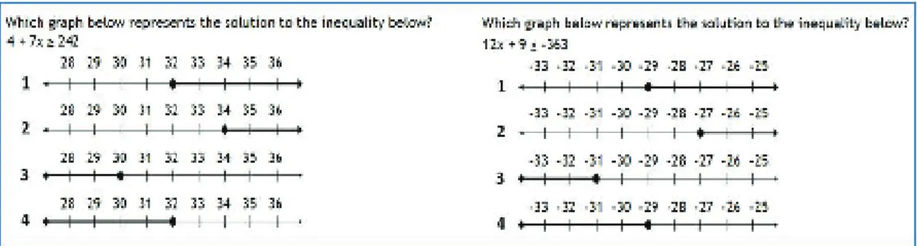
Mastery assignments require a large question bank from which to select problems to give the student. Item templates fill this purpose while reducing the content creation time. A template is a skeleton or variable form of a problem. For example, a question might ask a student which number line represents the solution to an inequality. In this case the inequality might be of the forma+bx≥kb+a, where a, b and k are integers. The solution to this problem will be a range starting from an integer and ending at infinity. Multiple number lines can also be generated which provide possible solutions to these problems. Figure 1 provides two potential problems that are instantiated or generated from this template.

Figure 2.1: An example of two problems in ASSISTments that are from the same item template. An item template provides a skeleton form for a question, and allows large question banks to be created with low content development time. An item template can also make a skeleton form for tutoring.

To reduce the number of unique problems that we will analyze, we will assume that all questions which are instantiated from the same item template are equal in difficulty, and the amount of learning that results from answering them. The item template can also provide a skeleton version

(14)

of tutoring. This allows the generation of question specific tutoring from the same item template. For figure 1, this means that for the first generated problem, this skeleton version of tutoring will solve the equation 4 + 7≥242 and in the second generated problem, it will solve 12x+ 9≤ −363. Similar to the problems generated from an item template, we will treat all tutorial feedback that has the same form to be equivalent.

2.4 Automatic Reassessment and Relearning System (ARRS)

ASSISTments contains a new feature which takes ordinary mastery assignments and, through a process of reassigning those assignments, allows students knowledge and long term retention rates to be tracked. This system is called the Automatic Reassessing and Relearning System (ARRS), which worked its way into ASSISTments at the end of the 2009-2010 school year. Instead of calling a student mastered when she complete an assignment, the student is given an initial mastery level of zero. Then after a set number of days (depending upon their mastery level) have passed, the student is presented with a random question from that assignment, on what we will refer to as a retention test. This test checks to see if the student has retained what she has learned during completion of the assignment.

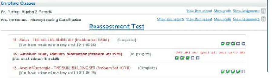
If the student answers correctly on the reassessment test, his mastery level for the assignment increases by one. If he answers incorrectly, his mastery level remains the same, and he has to relearn the assignment. Relearning is defined as completing the assignment after answering incorrectly on a reassessment test. The student finishes ARRS for the assignment when their mastery level reaches a teacher specified parameter, which defaults to four. 2.4 shows three assignments for the given student. The student only needs one more correct answer for the area of rectangle assignment to complete the reassessment cycle. If a student continuously answers their reassessment test incorrectly, they will never complete ARRS.

Towards the top of 2.4 are the two classes a student is enrolled in. To take her reassessment test, the student may click on the Reassessment Test link under the class called Mastery Learning Extra Practice. The student may also view their assignments by clicking on the Show Assignments link to the far right of the class name. When this page is loaded, the student will see assignments similar to the three shown in red in the bottom of figure.

(15)

Figure 2.2: A typical view of classes that a student is enrolled in. For the mastery learning class, the student can take their reassessment test, or can complete one of their assignments, shown in red. The checkmarks next to an assignment name indicate the mastery level of the student.

The ARRS system tests and retests students on a particular topic. The student is first presented with a mastery assignment, which they must complete to continue. They then are reassessed at varying intervals until they are able to answer correctly a week later, two weeks later, a month later and lastly two months later. A student only moves from one time interval to another if they answer correctly on the reassessment test. For each incorrect answer on a reassessment test, the student will have to complete the mastery learning assignment again, and be reassessed again at that same interval. Therefore, in order to proceed through the system, the student needs to retained the knowledge gained from the mastery assignment, and answer correctly when reassessed.

This dataset offers more data per student than an ordinary mastery learning assignment, a valuable asset in educational data mining, but it has this non uniform distribution of student responses. The perfect student will answer three correct in a row on his mastery assignment, answer correctly on his reassessment test a week later, and progress to the two week retention interval. Two weeks later, he will again see a question from this mastery assignment and answer it correctly, moving onto the month long retention period. After answering his reassessment test correctly a month later, his final hurdle is answering a question correctly two months after that. Since he is perfect, he answers this question correctly.

In the same class is another student, Sally, who is almost as smart as this perfect student. She does exactly what he does until the two month reassessment test, where she makes a mistake and answers incorrectly. She then has to go back and relearn this assignment, and it may take her three questions, six questions or even ten questions in order to get three correct in a row. Two months

(16)

later she gives her second attempt at the two month retention interval and this time she answers correctly.

These two students show some of the variance in this ARRS dataset. Sally may just of easily taken fifteen questions to initially complete the mastery learning assignment, or took four attempts to answer correctly on a reassessment test for the two week time interval. In order to analyze this dataset, models need to be able to handle arbitrary length sequences associated with different students progressing through the system. In addition, good models will leverage which retention interval the student is currently working towards.

Over five school districts used ARRS in its first year of deployment. Many teachers use it to make sure their students have the prerequisite skills upon entering their current grade. Since the teachers lack the time to review these prerequisites in class, they place them into this system and have students work though these recurring assignments for homework. These teachers like the system and view it as an aid rather than an intrusive research generation tool. However, by testing if students retain knowledge, its datasets can be used to model the long term learning gains that cognitive models discover.

(17)

Chapter 3 Methods and Data Manipulation

We analyze data using a dynamic Bayesian network which tracks student knowledge as they progress through items. This model identifies the learning each item causes as well as the effective-ness of tutorial feedback given to the student. This learning is quantified in a learn rate which is defined as the probability a student will now understand and have the necessary knowledge to solve a similar problem, after having completed a problem. However, due to scarcity in the datasets on particular items, accurate parameters cannot be learned for each problem. This is due to the size of the current datasets in relation to the number of items, and is not due to a limitation of the Bayesian network technique. However, by representing an item by the item template from which it was generated, accurate parameters are learned for each item template. Instead of a learning rate per question, we can have twenty questions generated from the same item template sharing the same learning rate.

In this work we measure the effectiveness of various types of tutorial feedback using a Bayesian network approach. We review the work done in [11] and show the effectiveness of various adaptations to this model. In the second part, we attempt to identify the ability of the model to determine student retention rates, and at the same time, validate the model as causing either short term or long term learning. We will also explore other factors which influence student retention.

In the first part of this paper, we attempt to learn the effectiveness of different types of tutorial feedback. In order to minimize any outside learning, we chose to analyze only the responses of a student on a mastery assignment the first day he worked on it. We found most students answered at least three questions (though some students did not complete the assignment) and few students

(18)

answered more than ten. Since at a minimum, students answered three questions, all reported results are based on the first three responses of each student. In subsequent research we found the results of looking at the first ten questions to be highly correlated with the results of looking at the first three. This analysis also discovered that datasets in which students end with three correct in a row, have higher learn rates than ones in which all students complete the same number of questions, but the relative difference between the different learn rates are highly correlated.

Since we are comparing the effectiveness of tutorial feedbacks, we are interested in the type of help given to the student. For each experimental problem set, all item templates within that problem set were designed to have two types of tutorial feedback. Although there may be six different templates that generated the problems in the problem set, there are only two distinct types of tutorial feedback amongst those items. This allows us to identify the item a student received by the type of help that was assigned to them.We did not have enough data to analyze the combination of the pairing of the item template that generated the question and the type of help given on the question, although we believe it to be an interesting analysis.

3.1 Tutorial Feedback

The experiments aimed to determine if the same material and tutoring strategies were presented in different ways, would there be a dramatic and significantly significant difference in learning. For example, one experiment attempts to identify a measure of cognitive overload. It compares presenting a full solution to the student, called a worked solution, to that same solution presented one step at a time. For low knowledge students presenting one step at a time helps, but for high knowledge students, we found that just giving them the procedure was enough to cause learning. For these students, even presenting them with a worked example, or a solution to a similar problem, was just as effective. The problem sets and types of tutorial feedback are shown in table 3.1. [14, 8, 15] The skills represented were finding percents, ordering fractions and decimals, and two step equation solving. Experiment 1 consists of problems with ordering positive and negative fractions and decimals. The tutoring has the student convert each fraction to a decimal and then asks the studentto order the corresponding decimals. In both conditions, the tutoring is broken down into three steps. In one condition, the student is told what to do on each step and just has to select a

(19)

Table 3.1: Five experiments were embedded into mastery learning problems sets. Each experiment compared the effectiveness of the tutorial feedback in Condition A with that in Condition B.

Experiment # Condition A Condition B Subject Matter

1 Solution (Steps) TPS Ordering fractions and decimals

2 Solution Worked Example Finding percents

3 Hints TPS Equation solving (Easy)

4 Solution (Steps) Solution Equation solving (Medium)

5 Solution (Steps) TPS Equation solving (Hard)

box stating they are ready to move on. In the other condition, tutored problem solving (TPS), the student is asked to input the answer to each step.

Experiment 2 deals with finding percents. In condition A, the tutoring consists of a worked out solution, while the second condition the student the same form of the solution, but its to a different question. Students are exposed to the same methodology, or procedure of solving, but they differ with the actual numbers of the problem.

The remaining three experiments are on equation solving. Experiment 3 compares hints that show the algebraic steps to solve the problem, with TPS. For example, the first step of TPS asks the student which number we need to add or subtract from each side to isolate the variable term on the left hand side. It then asks the student to identify how to arrive at a coefficient of one on the variable by selecting from four possible equations written in algebraic form. Lastly the student is asked to solve the original question. The hints in this experiment are similar, but start of with general guidance to solving the problem, and then show the steps without any explanation.

Experiment 5 seeks to answer the question of is it better to tell the student, or ask them how to do it. For both conditions, the help breaks solving the given equation into three steps. In the broken down solution condition, the user is asked to click that they see how the step is performed. In the TPS condition, the steps are the same, except the user is asked to select which operation was performed or to solve for the variable by dividing both sides by the coefficient of the variable.

3.2 Traditional t-tests and the Item Effect Model

We used two different procedures for analyzing which tutorial feedback is more affective. The traditional approach viewed the data as a pre and post test design and used a t-test to analyze learning gains due to the help seen on the first question. Since students are marked incorrect

(20)

once they see help, we only looked at students who answered the first question incorrectly. For these students, their response pairs to the first two questions were either incorrect then correct, or incorrect then incorrect. By splitting a student response pair by the type of feedback the question gave, we were able to analyze two different populations of learning gains, one for each type of tutoring. This approach only uses a small portion of the dataset, which by its nature, is not designed to be easily analyzed.

The other approach used a variant of the Item Effect Model, which is based on a Bayesian theory called Knowledge Tracing that assumes a student either possesses or does not possess the necessary knowledge to answer a question [6, 5] . In our context, this knowledge refers to a single skill, and we will use having the required knowledge and knowing the skill interchangeably. Since this required knowledge is not observable, we will refer to it a hidden or latent variable. The model estimates the students knowledge based upon the models parameters and the responses of the user on questions. There is a certain probability that by answering a question, a student who does not have the skill will gain it. This is referred to as the learn rate.

This theory still allows for a student to guess the answer if they do not have the skill, and to make a mistake even if they do. Formally knowledge tracing has four parameters. These are the initial probability a student knows the skill (L0), the probability they student transitions from the

unlearned state to the learned state (T), the guess rate, or probability a student answers correctly given they do not have the required knowledge of the skill (g0), and the probability they slip, or

answer incorrectly given they have the required knowledge of the skill (s0). We will be primarily

concerned with the different learning rates of questions.

A common assumption that we adopt is that once a student has a skill, they do not forget it. Our datasets are from the first day a student works on an assignment. Allowing a student to forget the skill is more accurately described as the student never having known the skill. In this sense, allow a student to forget may cause a better fitting knowledge, but goes against the idea of a cognitive model.

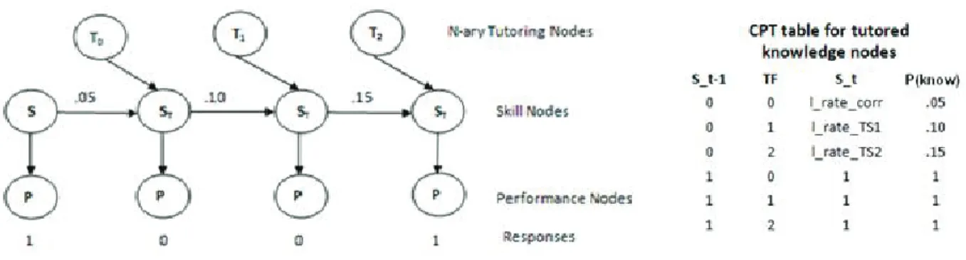
The Item Effect Model, shown in the bottom left of 3.2 differs from standard Knowledge tracing mainly by introducing the idea of students learning different amounts depending upon the question. There is a (Ti), for each question (qi), instead of just a single learning rate for all questions.It also assumes that some questions are easier to guess on, and other questions are easier to make mistakes

(21)

Figure 3.1: An example of a three problem topology for Knowledge Tracing and the Item Effect model including the associated parameters. The Item Effect Model learns additional parameters for each different item template in the problem set.

on. By introducing these additional per question parameters, the Item Effect Model has been shown to outperform standard knowledge tracing. [12] Our Item Effect approach consists of analyzing up to the first three questions each student answered. To detect significance, we divided the dataset into ten distinct equally sized bins. If both conditions caused the same amount of learning, the bins would follow a binomial distribution withn= 10 and p= 1/2. For a significant finding, we require the same tutorial feedback that has a higher learn rate when all the data is analyzed, to have a higher learn rate in eight of the ten bins.

In the educational data mining community, the two most common fitting procedures for Bayesian networks are expectation maximization (EM) and grid search. EM maximized the log likelihood of the observed events by adjusting its parameters in an iterative procedure. Grid search searches over the parameter space by testing all possible sets of parameter values at a certain precision increment, and selecting the set which minimizes the log likelihood or other error metric. In our work, we use the Expectation Maximization procedure due to the increased number of parameters in our model.

(22)

3.3 Findings from Previous Work

In [11], we looked at the effectiveness of various types of feedback from questions within mastery assignments by using both t-tests and the Item Effect Model.We ran five experiments that we embedded into mastery assignments at the beginning of the academic year.These experiments were discussed earlier and are shown in 3.3. The students were not placed into conditions and then given exclusively one condition, but rather were given one question at a time, with that question being randomly assigned either condition A or condition B. It was not uncommon for a student to receive both conditions multiple times in the same assignment.

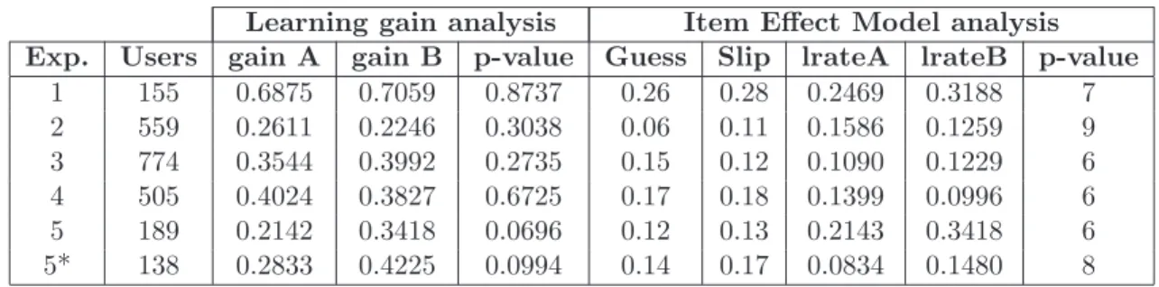
Table 3.2: The results of comparing the Item Effect Model vs. t-tests to determine the effectiveness of various methods of tutorial feedback within mastery assignments.

Learning gain analysis Item Effect Model analysis

Exp. Users gain A gain B p-value Guess Slip lrateA lrateB p-value

1 155 0.6875 0.7059 0.8737 0.26 0.28 0.2469 0.3188 7 2 559 0.2611 0.2246 0.3038 0.06 0.11 0.1586 0.1259 9 3 774 0.3544 0.3992 0.2735 0.15 0.12 0.1090 0.1229 6 4 505 0.4024 0.3827 0.6725 0.17 0.18 0.1399 0.0996 6 5 189 0.2142 0.3418 0.0696 0.12 0.13 0.2143 0.3418 6 5* 138 0.2833 0.4225 0.0994 0.14 0.17 0.0834 0.1480 8

We see that even with only using a small amount of data, the two methods agreed with each other in five of the six experiments. A significant finding was found for Experiment 5. However, it was discovered as a direct result of this finding that the significantly worse tutoring strategy contained a typo which told the students the wrong answer. This was later corrected and formed a new version of the same experiment. Although our model is unable to detect a significant difference in this experiment with users from when this typo was corrected onward, there is strong evidence to suggest that this typo effect may not have been the main cause for the original finding. This demonstrates that requiring a student to answer each step in equation solving is more beneficial than simply presenting them with the solution

This comparison provided justification into using the Item Effect Model to analyze actual stu-dent logs by showing that it agreed with a method (t-test approach to learning gains) that is widely used. In the remainder of [11], we showed how to look at student log data in such a way that it appears to have been designed as a randomized controlled experiment. The two main results of that paper are the idea of making use of the millions of unutilized student logged data records

(23)

using data mining techniques, and to show the Item Effect Model works with actual student data. Having established this, we are free to use this model to analyze other types of datasets.

(24)

Chapter 4 Further Method Explorations

Knowledge tracing is the simplest dynamic Bayesian network that can track student knowledge over timesteps. It is comprised of a latent knowledge node, and an observed performance node. Even with this simple consistency, it forms the basis of progressing students through the Cognitive Tutor, the largest intelligent tutoring system in the United States. This system treats all questions of the same skill as equivalent. In this sense, it has no notion of a question identity, and no sense of the relative difficulty of effectiveness of questions. To account for having only one learn rate for all questions of a given skill, the Cognitive Tutor tracks approximately 3000 different skills. The idea of an item template in ASSISTments, or a particular form of a question pertaining to a given skill, may exist as a skill in and of itself in the Cognitive Tutor. However, this is often not the most accurate representation of questions.

For example, consider three different item templates that are related to equation solving. In the Cognitive Tutor, each one of these three item templates may relate to one of its 3000 skills. When knowledge tracing is applied, a student will have a probability of knowledge associated with each one of the skills corresponding to these three item templates. However, since they are all equation solving questions, if a student knows one of them, he is more likely to know the other two. Independence among the three item templates can not be assumed. Conversely, if the three item templates are tracked as one skill, the knowledge tracing model will ignore the relative difficulty among these three item templates, and treat their difficulty and learning rate to be equivalent. The Item Effect Model addressed this issue by allowing for these three templates to be equivalent as a skill, but to vary in difficulty and learning rate. A similar argument could be made on the

(25)

shortcomings of treating questions answered on different days as equivalent. Therefore, adapting a model to maintain an item template has grounding, but yet itself is just one specific example of capturing more of the variance in student responses.

In this chapter we explore improvements to the model of detecting the effectiveness of various type of tutorial feedback by using more data about the students and the questions. Instead of using just the student performance and item template, we consider system wide user performance and look closely at the type of tutoring the student actually received. We compare the models on predictive accuracy under various metrics. We are primarily interested in modeling a pedagogical correction to the model, which states learning rate for an item should not be determined by the tutoring received if the student answers correctly and is not exposed to the condition. Remember that in ASSISTments, a student who is marked correct could not have been exposed to any type of tutorial feedback. We first exhibit this model and the other possible improvements, and then show the results of their predictive accuracy. Lastly we comment on the convergence behavior of the model under different topologies.

4.1 Correct Response Explicitly Modeled

To explicitly model a student answering correctly, we use a variant of the Item Effect Model in which we explicitly model the difference between learning from answering an item correctly and viewing confirmation of the correct answer, and learning due to tutorial feedbacks. In the model, the measure of student knowledge is dependent upon the knowledge of the student at the prior state (the previous question they answered) and the tutorial feedback given on the previous question. By modeling this tutorial feedback effect as a multinomial node taking on one more value than the maximum number of possible tutoring strategies, we can associate this extra value with a correct response on the previous item. This means that if the student did not get exposed to one of the types of help, we do not arbitrarily assign them to a condition for that item. In theory, this model allows us to make explicit the difference in effectiveness of various tutorial feedbacks.

This model makes the assumption that there can be a difference in learning rates depending on if the student answers correctly, and is not exposed to tutoring, and if the student answers incorrectly, and the type of feedback given for the item. There is an amount of learning associated

(26)

with seeing the main question, and a separate amount of learning associated with seeing the tutorial help. Although there is still some obfuscation in that only students who answer correctly do not see help, this could be fully realized by having a tutorial feedback which simply tells the student their answer is wrong and progresses them to the next item.

For an interpretive model, we would like the learning associated with seeing tutorial help in addition to the main item to be larger than just seeing the main item. Stated alternately, we would like students to learn more when they answer incorrectly and are given help. To reduce the number of parameters in this model, we assume that the same help on different items causes the same amount of learning. The different item templates all share the same parameters, which mitigates any intrinsic differences in their relative difficulty.

Unlike the current implementation of the Item Effect Model used in [11], this model does not model all possible sequences through a set of items or a set of tutorial feedbacks. Instead, any alterations to the original knowledge tracing model are localized in a specific node which represents the tutorial feedback received, the template of the current item or even a different factor such as a discrete interval of time spent on the current problem. We represent in our model the tutorial feedback used in the previous time step by an incoming arc to the knowledge node of the current time step. This node is a multinomial, taking on one more value than the maximum number of tutorial feedbacks in the dataset.

A benefit of this model is that all questions share the same guess and slip parameters. These shared parameters are pedagogically important, as we would expect students to guess and slip at the same rate regardless of future feedback to be received; i.e. this model is causal in this way. Moreover, using equivalence classes, the same item can appear in multiple places and share these same parameters, allowing for a smaller parameter space and potentially more accurate models with smaller datasets.

A significant advantage of using this topology is the ability for the model to scale. There is not one sequence per ordering of the tutorial feedback received, but rather one sequence for the maximum length user response sequence with an extra node that represents all possible types of feedback for that time step. For example, for sequences of length four, this model has eleven nodes, with three taking on three values, and the remaining eight taking on two values. For the adapted Item Effect Model used previously, we could potentially have sixteen sequences of eight nodes each.

(27)

Another benefit of having fewer nodes in our network is faster convergence rates. In some cases, this new topology will converge to very similar parameters twice as fast.

Figure 4.1: The Tutorial Effect Model with a sample set of student responses; correct, incorrect, incorrect, correct (1,0,0,1).

This new model with four questions is shown in 4.1. We see that after a correct answer, the student always receives T0 which is to signify the previous item was answered correctly and no

tutorial feedback was seen. We remark that our model has the same initial knowledge node which is only affected by the prior of the dataset. Similarly, the performance nodes are unchanged from the Item Effect Model and all questions share guess and slip parameters. With equivalence classes we can model different guess and slips per questions, but this would either introduce a new node per time slice or modeling of individual sequences. We state that this can be done, but ignore it. The simulation studies and comparison of learn rates will be presented in the appendix for this model. We next state the other factors including bin splitting procedures and prior setting heuristics and their effect on predictive accuracy.

(28)

4.2 Splitting Students and Setting Priors

Recent work [13] introduced a further individualization into the knowledge tracing model. In this approach, each student is allowed to have both an individual learn rate and an individualized prior. This gives rise to the notion of one student entering a classroom or more appropriately, signing into an ITS with a higher probability of knowing the items presented to them, even before they have their first opportunity to learn. It was shown that this approach can reduce degenerate models, which are those models in which a student has a higher chance of answering correctly if they do not know the skill. Since preliminary explorations of our datasets have shown certain classes with a high percentage correct on the first item, as well as classes with a low percentage correct on the first item, we find motivation to explore this model. Our model is a simplification of the prior per student model. Instead of having a prior knowledge parameter per student, we will have just two prior parameters for all students. By reducing the number of prior knowledge parameters in our model, we will be able to learn accurate learn rates with less data per student. In our case, we will learn the parameters with fewer question responses by students.

In the model presented, we represent two distinct sets of students classified by their level of prior knowledge; or simply, how likely they are to answer a question when they first log into an ITS on a given day.One set corresponds to high knowledge students and the other to low knowledge students. We refer to these sets as knowledge classes. Intuitively, one expects the high knowledge students to answer correctly when presented with a new question on a possibly unknown topic. Examples include students who study ahead, or students who repeat a course. Both of these students are expected to have prior knowledge of the topic, and with high probability, can answer a question correctly. Since knowledge is again a latent variable in our model, heuristic splitting techniques need to be employed that are capable of placing students in a knowledge class when they start off an assignment.

4.3 Splitting Methods and Initialization for Prior Knowledge

Two different splitting methods are used to place a given student into one of the two knowledge classes. In order to easily implement this model into an ITS, we require that the splitting algorithm must be implemented at run time. In other words, we cannot place a student into a knowledge

(29)

class based upon their performance on future questions. We will not discuss special considerations for new students to the ITS, but remark that either a cold start procedure or some combination of the predictions from placing the student in each knowledge class can be used. For this analysis, we place these new students consistently into the same bin, and ignore any data we may have on them.

The first bin splitting procedure that we refer to as bin split 1, is based upon system wide performance on problems prior to starting the assignment. We include all of the non tutorial feedback questions for each assignment for a given student. For instance, if a student asks for help on question X and is subsequently presented with tutorial feedback questions Y and Z, we only include the students incorrect response to question X. Many times questions in tutored problem solving which break a question into smaller steps, i.e. questions Y and Z, are easier than the original question. Subsequently, counting these helper questions leads to a bias estimate by overestimating weak students abilities. We use the system wide average for all students who answered at least five questions, and set the remaining students to the system wide average.

The median and average for all students using ASSISTments is slightly higher than 60 percent. Therefore, the low knowledge class represents all those students whose average is below 60 percent. The remaining students including those who have fewer than five completed questionsare placed in the high knowledge class. This procedure ignores those students who get the first few questions incorrect, but who quickly learn and answer the remaining questions correctly. This type of student will be placed in the high knowledge class when they start out each assignment with low knowledge. However, the robustness of the model combined with other students who fit in their natural class allows for well fitting parameters to be learned.

The other procedure, bin split 2, attempts to capture the student who quickly learns but starts off every assignment answering incorrectly. Instead of counting all main questions a given student has completed, this procedure only counts the first question on each assignment. Similarly, the median system wide average for all students who have completed at least five questions with this restriction is 60 percent, although the average percent correct is only 49 percent. Those students whose average is 60 percent or less are placed into the low knowledge class, with the remaining students placed into the high knowledge class. If a student has answered fewer than five problems, we set their average to 60 percent when we place them into the high knowledge class. Both of

(30)

these procedures can be calculated at run time, as they are based on past data. A third procedure could attempt to look at a students first response on a question of a given skill, although we were restricted in this attempt by a low system wide skill tagging percentage. Simply put, not enough problems are tagged with a given skill in our datasets.

Once students are classified as belonging to one of the two knowledge classes, our model still requires two prior parameters corresponding to these classes. For our model, we wanted to know the effectiveness of fixing the prior knowledge parameters for each knowledge class using other system information on the students in each knowledge class. The model is capable of learning these prior knowledge parameters through its fitting procedure, expectation maximization, but these learned parameters will maximize the log likelihood of the observed data, instead of modeling the data as accurately as possible. The aim here is to see the effectiveness of the model when we put a restriction on its parameters space, which is to say, the prior knowledge parameters are fixed. To fix these two parameters, we employed two prior parameter setting procedures, which initialized the prior for each knowledge class using a heuristic. System average, the first fitting procedure, averaged each students system wide performance according to the bin splitting procedure and initialized the prior to that amount. The other procedure, actual average, set the prior to the students average on the first question in the current assignment. Although this appears to look at the data, our evaluation method uses cross validation and tests against a test set that is not viewed by this procedure.

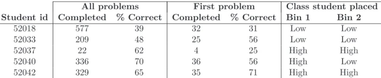
4.3 shows an example of the metadata collected for each student. The columns labeled Bin Split 1 correspond to all the problems the student completed in the system prior to their data collected on the given assignment. The columns labeled Bin Split 2 correspond to the students performance on the first problem of each assignment. Student 52037, is placed in the high knowledge class for Bin Split 2 since she completed only four problems, but her average of twenty five percent correct may suggest a low knowledge student.

Once the students are placed into bins, we need to set the prior for each class. Table 3 shows the initialization values for a single knowledge class, where the column labeled system performance is their percent correct from one of the two bin splitting procedures. Students 52037 and 52042 appear in this knowledge class, indicating this is sample data corresponding to high knowledge students using Bin Split 2. Since student 52037 answered fewer than five problems, his system statistic is set at sixty percent. The columns initial system average and initialize actual average

(31)

Table 4.1: The statistics for five sample students are shown under the two bin splitting procedures. The last two columns show which knowledge class each student would be placed in for each of the splitting procedures.

All problems First problem Class student placed

Student id Completed % Correct Completed % Correct Bin 1 Bin 2

52018 577 39 32 31 Low Low

52033 209 48 25 56 Low Low

52037 22 62 4 25 High High

52040 336 70 36 56 High Low

52042 329 65 35 71 High High

show the prior knowledge value that would be set if all students up to the current row were included in the knowledge class. For the first row, only the first students average contributes to these, where as in the last row, all students contribute. This is only shown here for clarity on the procedure used. In implementation, these two initialization values are calculated with all students of the given knowledge class.

Table 4.2: Example of five students and using their statistic from Bin Split 1 to seed the prior knowledge for the high knowledge class.

Student Statistics

Student id System stat. Correct q1 Init. system avg Init. actual avg

45620 85 0 85 0

48781 100 1 93 50

52037 60 1 82 67

48782 63 1 77 75

52042 71 1 76 80

The intuitive approach for using these initialization values lies in assuming the guess and slip values for the model are similar. If we assume they are equal, the number of students who have the required knowledge and answer incorrectly will be offset by those who do not have the knowledge, but who guess correctly. By using the actual average of the students performance on the first question, we should be able to better fit our training dataset as we are using the true prior.However, work [3, 4] has shown that various sets of parameters can fit and predict Knowledge Tracing models equally, while pedagogically representing very different characteristics. Therefore, we cannot expect a better fitting model, but we should expect the parameters found by the model to fit with our domain knowledge. By using these classification methods and heuristic starts, we are in effect leading our model into a certain parameter range, which is similar to work done with contextual

(32)

guess and slips and Dirchilet distributions [2]. In these other approach, instead of fixing a parameter based on heuristics or domain knowledge, the model tends to toward certain parameters as a distribution is placed on a parameter, which in effect, limits how far that parameter will vary, as this distribution makes it increasingly less likely that it move further from its believed mean.

4.4 Metrics for Accuracy

Different metrics are used in the literature to measure the accuracy of a model. In some cases we are interested in a binary prediction, either zero or one, in which case area under the curve or AUC is often used. This metric is a measure of the number of swaps needed to order the predictions in such a way such that all predicted values that correspond to actual values of zero, are sorted before any value that is actually one. A value of one is a perfect prediction, and a value of zero is the opposite of a perfect prediction. Any other score is a measure of the skewness of the predictions. Other areas are interested in minimizing our total error, which is commonly expressed as either the root mean squared error (RMSE) or mean absolute error (MAE). Our fitting procedure, expectation maximization uses log likelihood measure to determine which parameters cause the observed data with the highest probability. In this work we are interested in prediction, as if we can accurately detect students who answer correctly, we can give less problems to them, and similarly, students who answer incorrectly, can be given some type of intervention prior to more reassessment.

Our model makes predictions for all students, with the differences in the predictions arising from the knowledge class of the students, the types and ordering of tutorial feedback the student receives, and the performance of the student. The tutorial feedback and performance of the student is observed, while the knowledge class of the student is set using heuristics. Since as an ITS we do not want to change a students path before we have information about their knowledge in a given domain, we do not attempt to model the accuracy of the first question. We only predict a students second and third responses.

Root mean square error measures the square of the differences between the predicted per-formance of a student, a continuous measure from zero to one, and the actual perper-formance of the student, a binary zero or one. Since the difference is squared, a few large deviations can equal many smaller deviations. A common measurement of the predictive accuracy of a model is to compare it

(33)

to selecting the value that minimizes the square of the deviations. For example, if 70 percent of the responses are correct, a base model is one that maximizes.7∗(p(x)−1)2+ (1−.7)∗(p(x)−0)2, where p(x) is the predicted value. The model will always predict p(x). which in this case is 0.7.Taking the functions derivative can easily show this.

This metric also does not include information as if the model is receiving its score for predicting close to zero or close to one most of the time. Taking a dataset with half correct and half incorrect answers, a prediction of 0.75 which is close to 1receives the same score as a prediction of 0.25, which is close to zero. Identifying causes of RMSE often leads to multiple methods of prediction and ensembling , and will not be included. Mean absolute error is very similar to RMSE, except that it takes the absolute value of the deviations instead of square.

We will use five fold cross validation to test the accuracy of our model. The students in a dataset are be partitioned into five bins. To predict the responses of students in bin three, our model trains on the students responses from bins one, two, four and five. Using the learned parameters, it predicts the responses for each student in bin three. To predict the second question, we use the knowledge class of the student, the performance on the first question and the type of tutorial feedback on the first question. To predict the third question, we use the performance of the student on the first two questions and the type of tutorial feedback given on the first two questions. Using this procedure to predict student responses for bins one through five results in five different sets of predictions. We will refer to each one of these as a fold. We predict the entire dataset by combining the predictions from each one of the folds. This is referred to as the complete prediction for the dataset.

(34)

Chapter 5 Results

In this section we decide which model performs best at predicting students performance. We are specifically interested in the differences between the two bin splitting procedures, the differences between the heuristic setting procedures, and whether we should attempt to model a student answering correctly and not receiving any help.Since we have eight possible combinations, each run over five fold cross validation, we present aggregated information.The data used here is of the same format as??, except for it includes all data collected up until April 20, 2011. For all of the experiments, we have additional users. Experiment 5* will not be analyzed in this section.

5.1 Comparing Bin Splitting Procedures

The two bin splitting procedures attempt to identify students by either their overall performance, or their performance at the start of assignments. To compare the effectiveness of the bin splitting procedure, we are going to compare each with using the original model without explicitly modeling a correct response. We set each bin to the actual average of the students on the first question. We do this to reduce bias from having a population within a knowledge class not having done enough problems for the first response, and having their averages artificially set to 60 percent. The results are presented in 5.1.

Using all of the data for a student to seed a student into a high or low knowledge bin results in better root mean squared error, and mean absolute error. Although the two averages appear close, and differ only in the hundredth digit, RMSE using all data outperforms a students first

(35)

Table 5.1: Comparison of cross fold validation results for the two bin splitting procedures with prior set to average of first response. The last two rows state for the full prediction, how many times did each bin splitting procedure have the lower error rate.

Error Metric # times best in folds

Bin Split RMSE MAE AUC RMSE MAE AUC

1 All .4252 .3475 .7267 22 16 13

2 First .4272 .3497 .7219 3 9 12

Total 1 All .4217 .3475 5 3

Total 2 All .4236 .3497 0 2

response in twenty two out of the twenty five folds, and in all five of the complete predictions for the dataset. The metrics are close for predicting the second and third questions, but could accelerate in divergence as the number of predicted questions increases. Unfortunately, there is no concise better method for AUC. Setting knowledge classes by system wide average outperforms the first response by looking at the average AUC, but there is no distinction, thirteen vs. twelve for one procedure causing a larger number of test sets to be favorable.

5.2 Comparing Prior Setting Procedures

In this model we thus far have explored two distinct bin splitting procedures. In the prior section, we saw evidence thatshows using all of the students data results in better predictions. For comparing different prior setting procedures, we will adapt this bin splitting procedure 1that looks at all the student data and had shown to result in better RMSE. Like before, we will use the original topology of the model, and will not explicitly model a student answering correctly.

Table 5.2: The percentage correct for each of the five experiments by question. Percent Correct

Experiment Question 1 Question 2 Question 3

1 .7424 .8563 .8797 2 .4622 .4549 .5293 3 .4318 .5115 .5719 4 .3417 .4847 .5032 5 .2649 .4239 .5269 Total .4486 .5463 .6022

Both of the bin splitting procedures ignored the relative difficulty of the problem set in that they assume all questions a student answered should be equally weighted. In addition, if we use this

(36)

system wide performance to set the prior for an analysis, it assumes the dataset is representative of a mastery learning assignment in ASSISTments, which has on average, a 67 percent correct. If however our problems sets do not follow this pattern and are much harder, as shown in 5.2, our model will have to compensate, either through worse predictions, lowering the guess and rate and increasing the slip rate, or reducing the learn rate. These are all ways that a knowledge tracing model can adjust to too high of a prior and many early incorrect responses.

We would expect the procedure that sets students prior based upon their actual performance to the current problem set, to be more representative of these harder problem sets. 5.2 shows the students actual mean performance on the first question when Bin Split 1 is used, in the columns labeled Avg. Q1.Under high knowledge, this column represents the mean performance on each problem set for students whose system wide average was above 60 percent. This should be compared to the All column under system performance, which is the system wide average for the same students. For completeness, we also show the first response average for each knowledge class when bin split 2 is used, although we do not showing their corresponding mean performance on the first question of each problem set.

Table 5.3: Compares the actual percentage correct on each of the experimental problem sets to the mean of the students system wide percentage correct. We can tell that experiments 2 through 5 are much harder than an average question.

High Knowledge Low Knowledge

System Performance System Performance

Experiment Avg Q1 All First Resp. Avg. Q1 All First Resp.

1 .8273 .7373 .7624 .4127 .5334 .5030

2 .5861 .7278 .7286 .2909 .4542 .4548

3 .5197 .7421 .7554 .3025 .4750 .4503

4 .5388 .7148 .7424 .2015 .4277 .4243

5 .4527 .7223 .7279 .1666 .4840 .4648

Our high knowledge students, whose system wide average is in the seventies, was mostly found to be in the fifties. By fixing the prior knowledge parameter in our model to the student system performance average which is in the seventies, our model is in effect attributing a higher knowledge level to the students. Similarly for our low knowledge students, their actual performance on the first item was only about half of their system wide performance. Since two bin splitting procedures pro-duce nearly identical means, using the system wide performance does not seem indicative of actual performance, and therefore we would expect the difference error metrics to be very pronounced.

(37)

Table 5.4: Comparison of cross fold validation results for the two prior setting procedures when bin split 1 is used. The last two rows state for the full prediction, how many times did each prior setting procedure have the lower error rate.

Prior setting proc. RMSE MAE AUC RMSE MAE AUC

Dataset .4252 .3475 .7267 22 23 15

Mean system perf. .4234 .3602 .7208 3 2 10

Total dataset .4217 .3475 1 4

Total mean system perf. .4202 .3603 4 1

However, this distinction is not well pronounced in the results. This is a byproduct of a robust model adjusting to too high of a prior by altering its other parameters to make early mistakes more likely. The data suggests that the two procedures are relatively equal, with indication that it depends upon the metric used. In twenty three of the twenty five runs, fixing the prior based upon the percentage correct of the students first response in the dataset is best under mean absolute error, but is only better in ten datasets for mean square error. This could be indicative of the model using the system setting as predicting higher correct values for students who are making more mistakes in the test datasets. The RMSE errors are here large, but they still beat the baseline of guessing the average percent correct for each question. The high AUC (above .66) indicates that although the model is usually far off from the true result, it is giving students who tend to answer incorrectly a lower prediction than students who answer correctly, which is acceptable and wanted for binary predictions.

5.3 Comparing Modeling Correct Response

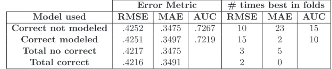
In the model presented in [11], students who did not see any help are still attributed to the help that they were randomly assigned. By explicitly modeling students not seeing help, we hoped to improve our accuracy of predictions, as well as find closer to the true parameters of the model. To determine if modeling this pedagogical correction of not attributing a student to seeing help unless they viewed such help, we will use Bin Split 1 and will seed the priors based upon the mean performance of the first question for each of the experiments. 5.3 shows the errors associated with predicting students in five fold cross validation. From this, we can see some mild evidence to suggest that modeling correct may be warranted, but it is not appear enough to adjust the original model.

(38)

Table 5.5: Comparison of cross fold validation results for the adapted Item Effect model with and without a correct response explicitly modeled.

Model used RMSE MAE AUC RMSE MAE AUC

Correct not modeled .4252 .3475 .7267 10 23 15

Correct modeled .4251 .3497 .7219 15 2 10

Total no correct .4217 .3475 3 5

Total correct .4216 .3491 2 0

The two models presented here are identical in topology (and differ in this respect to the Item Effect Model) and number and type of parameters except for this extra learn rate for answering a question correctly. The two models find near identical parameters (simulated datasets and item template datasets appeared very similar), although certain patterns emerge. For each of the five folds, the learned guess rates differ usually by 5 percent, but for the easiest problem set, in Exper-iment 1, this difference rises to 20 percent. The slip values difference is usually smaller, between one and five percent, but rises to 9 percent for Experiment 1. The higher slip values are always associated without modeling the correct node. Similarly, in four problem sets high guess values were also associated with this model. However, this difference in guess rates is mitigated when all the entire dataset is analyzed, which indicates it is an artifact of the particular splits.

Generally higher guess and slip values are either to be taken as that the problems were easy to guess and make mistakes on, or as less accurate student knowledge predictions. If the model is less certain about a students knowledge, they need to allow for a larger variation in responses by increasing the performance guess and slip parameters. Often in practice, these parameters are bounded by domain knowledge, which can be implemented through assigning distributions to them or by using a different fitting procedure such as grid search.

Another commonality among the learned parameters is high learn rates associated with tutoring, and low learn rates associated with answering correctly. By answering a question correctly, the belief about a students knowledge should increase. This can be interpreted either as a student learning and gaining the acquired knowledge, or the model detecting the student had the knowledge with the correct response serving as evidence supporting this claim. Although one might expect a high learn rate to be needed for the model to detect the student has the required knowledge with high probability, a sequence of correct answers with a low learn rate can produce the same result. A model that has a prior of 30 percent, a slip rate of 10 percent, a guess rate of 15 percent, and a learn