Application and development of advanced engineering geographical information systems for pipeline design

C O P Y R I G H T

Attention is drawn to the fact that copyright of this thesis rests with the author. A copy of this thesis has been supplied on condition that anyone who consults it is understood to recognise that its copyright rests with the author and that they must not copy it or use material from it except as permitted by law or with the consent of the author.

Application and Development

of Advanced Engineering

Geographical Information Systems

for Pipeline Design

Herbert Keith Winning

A thesis submitted in partial fulfilment of the University’s

requirements for the Degree of Doctor of Philosophy

Coventry University

Buckinghamshire New University

May 2015

Abstract | i

Abstract

This thesis proposes the use of an Advanced Engineering Geographical Information System (AEGIS) for the improved design of onshore pipelines, from concept to operation. The system is novel in that it is function rather than discipline or software specific.

The thesis statement has been developed, and an aim and set of research objectives identified (along with the success criteria for the evaluation of the system), based on a review of current pipeline design methods.

Drawing on a design science research methodology (DSRM), the thesis proposes the development of the system as an artefact in order to validate the proposed constructs, models, methods and implementations. The thesis discusses the underlying issues of data interoperability, the application of open data standards, and the integration of computer aided design (CAD) and geographical information systems (GIS). These challenges are addressed in the thesis and demonstrated through the implementation of the system.

To support the development of the system, research was undertaken in the fields of pipeline engineering, environmental engineering and engineering design. As part of this research, a number of peer-reviewed journal papers were published, and conference papers presented in Kampala, Houston, London and Split. These papers covered the key fields contained in the thesis including, fluid mechanics, bio-systems engineering, environmental engineering, CAD/GIS integration (CGI), and the application and development of geospatial pipeline data models.

The thesis concludes that the approach is valid, offering significant improvement across all fields compared to the current method of pipeline design. By taking a functional approach to the challenges of the design of pipelines, a system has been developed that addresses the requirements of the pipeline engineer, environmental engineer and engineering designer. The system enables the user to select the software of their choice, thereby reducing the problems associated with data interoperability, retraining and system integration. The sharing of data and outputs from analysis carried out within the system, provides an integrated approach, which can subsequently be used for the integrity management of the pipeline during the operational phase of the project.

The scope for further development of this approach to pipeline design is also discussed. In addition to the inclusion of further engineering and environmental analysis, there is the potential for using the system for the design of subsea pipelines.

Preface | ii

Preface

This thesis integrates elements of pipeline engineering, environmental engineering, engineering design, computer aided engineering (CAE), CAD, and GIS to provide an advanced engineering geographical information system for pipelines. While the approach is equally applicable to both onshore and offshore pipelines, the thesis focuses on the application to onshore pipelines.

Chapter 1 introduces the fields within which this research applies. A brief overview of the historical development of onshore pipelines provides temporal context, while the following sections introduce the engineering, environmental and design issues. As the data for the model matures and becomes available at different phases of the project, an overview of the construction and operational phases of the project are also given.

Chapter 2 presents the research question, scope of the research, and sets out the aim, objectives and the success criteria for the thesis. Crucially it introduces and defines the concept of the AEGIS. The key areas for research are identified and the scopes defined for the supplementary literature reviews. These are presented in the respective chapters to which they apply.

Chapter 3 details the research methodology. The overall methodology of the thesis is outlined, together with the selected methodologies for the specific research areas of pipeline engineering, environmental engineering and engineering design (Chapters 4, 5 and 6) respectively. The methods selected for the design and evaluation of the AEGIS (Chapters 7 and 8) are also outlined.

Chapters 4, 5 and 6 cover the research in the fields of pipeline engineering, environmental engineering and engineering design with respective chapters incorporating an introduction, literature review, methodology, analysis and discussion of the topic.

Chapters 7 and 8 detail the development and evaluation of an instantiation of the AEGIS which is termed as the Pipeline Integrated Engineering Environment (PIEE), based on the Software Design Specification (SDS) in Appendix E. In this thesis, the terms AEGIS and PIEE should be read as synonymous.

Finally, Chapter 9 presents the conclusions of the thesis and identifies the aspects of the research that are novel or contribute to the canon of knowledge. Limitations of the current research and areas for further research are also discussed.

Acknowledgements | iii

Acknowledgements

I owe an enormous debt of gratitude to my wife Pat, for her unfailing encouragement, support and patience throughout the course of my studies. Balancing the requirements of part-time study with home and work commitments is not always easy, but it is those who support us, rather than the student, that give most and gain least, for as Robert Louis Stevenson said:

Perpetual devotion to what a man calls his business, is only to be sustained by perpetual neglect of many other things. (2009: 4)

I would like to thank my employer, CB&I Limited, for their financial support for attending conferences and my friend Dr Alistair Miller for reading the thesis; his suggestions and comments have helped to improve its clarity, and my thinking.

I would also like to record my gratitude to Dr Mike Hann, Professor Emeritus at Cranfield University, and one of the foremost experts on soil erosion for onshore pipelines. I have been most fortunate to be able to work with him in the field on a number of occasions; nobody could have had a better teacher and I thank him for his tutelage and patience in explaining the fields of soil mechanics and erosion.

All research students owe a tremendous debt to their supervisors and I have certainly been most fortunate in having both Dr Tim Coole and Dr Richard Mather as my supervisors; their guidance, encouragement and support have been instrumental in my getting to this stage. In particular, Dr Tim Coole has been my companion throughout my journey of enlightenment, a journey of almost nine years. He has given me perhaps the most precious gift a master can to his pupil: the conviction that my vision and ability is limited only by my diligence, endeavour, knowledge and desire to learn.

All men dream: but not equally. Those who dream by night in the dusty recesses of their minds wake in the day to find that it was vanity: but the dreamers of the day are dangerous men, for they may act their dreams with open eyes, to make it possible. (Lawrence, 2008: 23)

Finally, I would like to thank all the faculty staff, past and present. They have not only educated and supported me but have also fostered a keen thirst for knowledge that will remain with me always, and for which I am most grateful.

AEGIS, apart from being an acronym for Advanced Engineering Geographical Information Systems within the context of this research, is defined as:

An attribute of Zeus and Athene (or their Roman counterparts Jupiter and Minerva) usually represented as a goatskin shield.

(Oxford Dictionaries, 2010) Minerva1 _{is the Roman goddess of wisdom and sponsor of arts, trade and defence. Minerva} has a special meaning for me for numerous reasons. She embodies the virtues of the acquisition and pursuit of knowledge through adversity, and I have included her as she links both Buckinghamshire New University and Coventry University through their common motto of ‘Arte et Industria’.

1 _{The image is a detail from the Mosaic of the Minerva of Peace by Elihu Vedder, in the}

Declaration | iv

Declaration

I declare that this thesis and the work presented in it are my own and have been generated by me as the result of my own original research.

I confirm that:

1. This work was done wholly or mainly while in candidature for a research degree at this University.

2. Where any part of this thesis has previously been submitted for a degree or any other qualification at this University or any other institution, this has been clearly stated. 3. Where I have consulted the published work of others, this is always clearly

attributed.

4. Where I have quoted from the work of others, the source is always given. With the exception of such quotations, this thesis is entirely my own work.

5. Where elements of this work have been published or submitted for publication prior to submission, this is identified in Section 2.6 under the relevant chapter number, in addition to the references given at the end of the thesis.

6. This thesis has been prepared in accordance with the Coventry University Academic Regulations version 2014, Section 8 and the Chicago Manual of Style (sixteenth edition).

7. I confirm that if the submission is based upon work that has been sponsored or supported by an agency or organisation that I have fulfilled any right of review or other obligations required by such contract or agreement.

Herbert Keith Winning May 2015

Contents | v

Contents

F

M

Index of Tables ... xiv

Index of Equations ... xv

Index of Publications ... xvii

Nomenclature ... xviii

Glossary ... xxi

C

1

I

... 1

Development of Onshore Pipelines ... 2

1.1 Environmental Issues ... 5

1.2 Computer Based Design... 9

1.3 Pipeline Design ... 10

1.4 Pipeline Construction ... 14

1.5 Survey and Stacking (Stage 1) ... 14

1.5.1 Front-End Clearing (Stage 2) ... 14

1.5.2 Right of Way Preparation (Stage 3) ... 15

1.5.3 Stringing (Stage 4) ... 15 1.5.4 Bending (Stage 5) ... 16 1.5.5 Welding (Stage 6) ... 17 1.5.6 Trenching (Stage 7) ... 17 1.5.7 Coating and Inspection (Stage 8) ... 18

1.5.8 Lowering-In (Stage 9) ... 19

1.5.9 Backfill (Stage 10) ... 19

1.5.10 Tie-In and Testing (Stage 11) ... 19

1.5.11 Right of Way Reinstatement (Stage 12) ... 20

1.5.12 Pipeline Operation ... 21

1.6 The Challenge ... 21 1.7

Contents | vi

C

2

T

S

... 23

Review of Current Method of Pipeline Design ... 25 2.3 Literature Survey ... 28 2.4 Pipeline Engineering ... 29 2.4.1 Environmental Engineering ... 32 2.4.2 Engineering Design ... 33 2.4.3

Aim and Objectives ... 35 2.5 Aim ... 35 2.5.1 Objectives ... 35 2.5.2 Success Criteria ... 36 2.6

Advanced Engineering Geographical Information Systems ... 38 2.7

C

3

M

... 39

Review of Explicit Friction Factor Equations ... 47 3.2.1

Improved Method of Estimating Friction Factor ... 48 3.2.2

Determination of Location Class ... 49 3.2.3

Environmental Engineering ... 49 3.3

Engineering Design ... 50 3.4

Design and Development of the AEGIS ... 50 3.5

Evaluation of the AEGIS ... 51 3.6

C

4

P

E

... 54

Supplementary Literature Review ... 55 4.1.1 Analysis ... 58 4.1.2 Results ... 62 4.1.3 Discussion ... 63 4.1.4

Improved Method of Estimating Friction Factor ... 64 4.2 Approach ... 64 4.2.1 Analysis ... 67 4.2.2 Results ... 68 4.2.3

Contents | vii Discussion ... 71 4.2.4

Determination of Location Class ... 72 4.3

Supplementary Literature Review ... 72 4.3.1 Approach ... 76 4.3.2 Discussion ... 78 4.3.3

C

5

E

E

... 80

Soil Erosion ... 82 5.1.1

Erosion Control for Pipelines ... 84 5.1.2

Modelling Soil Loss ... 88 5.1.3

Determining the Individual Factors of the USLE ... 90 5.2

Rainfall Erosivity Factor (R) ... 91 5.2.1

Soil Erodibility Factor (K) ... 92 5.2.2

Slope Steepness (S) and Slope Length (L) Factors ... 93 5.2.3

Crop Management Factor (C) ... 94 5.2.4

Erosion Control Practice Factor (P) ... 94 5.2.5 Results... 94 5.3 Discussion ... 95 5.4

C

6

E

D

... 101

CAD/GIS Integration (CGI) ... 102 6.1.1

Data Interoperability and Open Standards ... 103 6.1.2

Pipeline Design and GIS ... 106 6.1.3

Discussion ... 108 6.2

C

7

D

AEGIS ... 110

Object Model and Classes ... 115 7.4.1

Abstract Classes ... 116 7.4.2

Feature Classes ... 117 7.4.3

Contents | viii Data Types and Data Dictionary ... 127 7.4.4 Methods ... 127 7.4.5 User Interface ... 128 7.5 Modelling ... 128 7.5.1

Design and Reporting ... 133 7.5.2 Core Components ... 134 7.6 Hydraulic Analysis ... 134 7.6.1 Location Class... 145 7.6.2 Environmental Engineering ... 150 7.6.3 Engineering Design ... 152 7.6.4 Discussion ... 165 7.7

C

8

R

E

AEGIS ... 167

Results and Evaluation ... 171 8.2

Static and Architecture Analysis ... 171 8.2.1

Black-box and White-box Testing ... 174 8.2.2 Optimisation ... 175 8.2.3 Dynamic Analysis ... 175 8.2.4 Simulation ... 176 8.2.5 Case Study ... 177 8.2.6 Informed Argument ... 179 8.2.7 Discussion ... 183 8.3

C

9

C

F

W

... 185

Limitations of the Research ... 190 9.2 Research Implications ... 192 9.3 Further Work ... 193 9.4 Conclusion ... 195 9.5

Contents | ix

R

... 196

Index of Appendices | x

Index of Appendices

Appendix A – Review of Explicit Friction Factor Equations ... 212

Appendix A1 – Reviewed Equations ... 212

Appendix A2 – Tables ... 227

Appendix A3 – 2D and 3D Contour Plots ... 231

Appendix B – Improved Method of Estimating the Friction Factor ... 245

Appendix B1 – Tables ... 246

Appendix C – Determination of Location Class ... 251

Appendix C1 – Extract from ASME B31.8-2012 ... 252

Appendix D – Soil Erosion Classification using Remote Sensed Data ... 254

Appendix D1 – WMO Data for Yevlax (Azerbaijan) ... 255

Appendix D2 – Vegetation Classification ... 260

Appendix D3 – Azerbaijan Aggregated Values by 1,000m Sections ... 262

Appendix D4 – Azerbaijan Aggregated Values by 500m and 250m ... 274

Appendix D5 – GIS Maps ... 275

Map 1 – Study Area Overview ... 276

Map 2 – Study Area Landsat Imagery ... 277

Map 3 – WMO Weather Station Locations ... 278

Map 4 – Vegetation Classification ... 279

Map 5 – Soil Classification... 280

Map 6 – SRTM Digital Elevation Model ... 281

Map 7 – Slope Analysis ... 282

Map 8 – Soil Erosion Risk Assessment (Azerbaijan) ... 283

Map 9 – Soil Erosion Risk Variance (Azerbaijan) ... 284

Appendix E – Software Design Specification (SDS)... 285

Appendix F – Code Sample (PIEE_PODS-Export) ... 472

Index of Figures | xi

Index of Figures

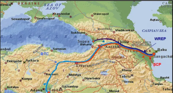
Figure 1.1 – BTC and SCP Pipeline Projects ... 4

Figure 1.2 – SCPX Pipeline Project ... 4

Figure 1.3 – Caspian Sea showing Eutrophication ... 6

Figure 1.4 – Free Spanning Pipe Due to Soil Erosion (Georgia) ... 8

Figure 1.5 – Gully Erosion in Highly Erodible Soils (Azerbaijan) ... 8

Figure 1.6 – Simplified Pipeline Design Flowchart ... 13

Figure 1.7 – Typical Pipeline Construction Sequence ... 14

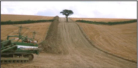
Figure 1.8 – Right of Way Preparation (UK) ... 15

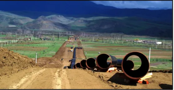
Figure 1.9 – Pipe Stringing (Georgia) ... 16

Figure 1.10 – Pipeline Bending (Georgia) ... 16

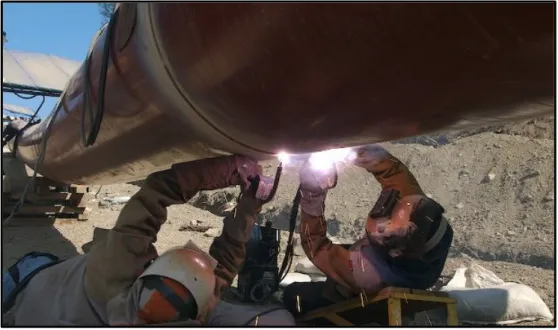
Figure 1.11 – Pipeline Welding (Canada) ... 17

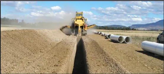
Figure 1.12 – Trenching (Australia) ... 18

Figure 1.13 – Field Joint Coating ... 18

Figure 1.14 – Pipeline Lower and Lay (Georgia) ... 19

Figure 1.15 – Hydro Testing (UK) ... 20

Figure 1.16 – Newly Reinstated Pipeline RoW (UK) ... 20

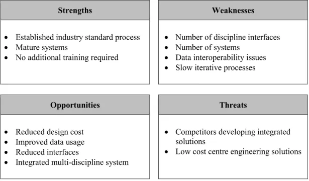
Figure 2.1 – SWOT Analysis of Current Pipeline Design Methodology ... 26

Figure 2.2 – AEGIS/PIEE Use Case Diagram ... 28

Figure 2.3 – Pipeline Engineering Literature Review Relevance Tree Diagram ... 31

Figure 2.4 – Soil Erosion Literature Review Relevance Tree Diagram ... 33

Figure 2.5 – Engineering Design Literature Review Relevance Tree Diagram ... 34

Figure 3.1 – Kuhn’s Scientific Revolution ... 41

Figure 3.2 – Research Framework in Information Technology ... 44

Figure 3.3 – Design Science Research Methodology Process Model ... 46

Figure 4.1 – Error Distribution Classification ... 60

Figure 4.2 – Error Distribution for Equation 4.6 ... 68

Figure 4.3 – Ranking Plot (Showing Equation Numbers) ... 69

Figure 4.4 – Ranking Plot (Showing Combined Rank) ... 70

Figure 4.5 – Normalised Plot for Accuracy and Computational Efficiency ... 71

Figure 4.6 – Distribution of Gas Pipeline Failure by Cause ... 74

Figure 4.7 – Ruptured Section of Pipeline (Texas 2010) ... 75

Figure 4.8 – Determination of High Consequence Area ... 78

Figure 5.1 – Erosion Types (Sheet, Rills and Gullies) ... 83

Figure 5.2 – Processes of Wind Erosion ... 83

Figure 5.3 – Double Wicker Fence and Rock Dam ... 85

Figure 5.4 – Stone Waterway and Diversion Berms (Hassan Su - Azerbaijan) ... 86

Index of Figures | xii

Figure 5.6 – Overview of the Variation in Erosion Risk Classification ... 95

Figure 5.7 – Typical Gully Erosion in Erodible Soils near Sangachal, Azerbaijan ... 96

Figure 5.8 – Area of High Erosion Risk (Azerbaijan - East) ... 97

Figure 5.9 – A 20m Diameter Gryphon at Location 3E ... 98

Figure 5.10 – Area of High Erosion Risk (Azerbaijan - West)... 98

Figure 5.11 – Comparison of Field and GIS Data in 1,000 m Aggregated Sections ... 99

Figure 5.12 – Modified GIS Calculated and Field Values 1,000 m Sections ... 100

Figure 7.1 – PIEE Project Phases ... 112

Figure 7.2 – PIEE Object Model ... 115

Figure 7.3 – PIEE Abstract Classes ... 116

Figure 7.4 – PIEE Model Feature Class ... 117

Figure 7.5 – PIEE Schedule Feature Class ... 118

Figure 7.6 – PIEE Offline Feature Classes ... 118

Figure 7.7 – PIEE Route Feature Classes ... 119

Figure 7.8 – PIEE Polyline Feature Classes ... 121

Figure 7.9 – PIEE Point Feature Classes ... 123

Figure 7.10 – PIEE Polygon Feature Classes ... 124

Figure 7.11 – Function Code Format ... 128

Figure 7.12 – PIEE AutoCAD Menu (PIEE Model Ribbon Tab) ... 128

Figure 7.13 – Model Panel ... 129

Figure 7.14 – Route Panel ... 129

Figure 7.15 – Route Panel, StationLine Drop Down List ... 129

Figure 7.16 – Route Panel, Profile Drop Down List ... 130

Figure 7.17 – Route Panel, ROW Drop Down List ... 130

Figure 7.18 – Route Panel, Intersection Points Drop Down List ... 130

Figure 7.19 – Route Panel, Aerial Markers Drop Down List ... 131

Figure 7.20 – Engineering Panel ... 131

Figure 7.21 – Engineering Panel, Pipe Segments Drop Down List ... 131

Figure 7.22 – Engineering Panel, Covers Drop Down List ... 132

Figure 7.23 – Feature Panel ... 132

Figure 7.24 – Topography Panel ... 132

Figure 7.25 – Topography Panel, Contours Drop Down List ... 133

Figure 7.26 – PIEE AutoCAD Menu (PIEE Design Ribbon Tab) ... 133

Figure 7.27 – Drawing Set Panel Template Drop Down List ... 134

Figure 7.28 – TemperatureContour.Import (ENG-P-008-01) Flowchart ... 135

Figure 7.29 – PipelineTemperature.Create (ENG-P-007-01) Flowchart ... 136

Figure 7.30 – PipelineHydraulics.Create (ENG-P-006-01) Flowchart ... 137

Figure 7.31 – IntPipelineHydraulics.Calculate (ENG-I-006-02) Flowchart ... 138

Index of Figures | xiii

Figure 7.33 – IntClassLocation.Calculate (ENG-I-004-02) Flowchart... 149

Figure 7.34 – SoilErosion.Create (ENV-P-003-03) Flowchart ... 151

Figure 7.35 – ReinstatementCode.Create (ENV-P-001-02) Flowchart ... 152

Figure 7.36 – Template.Create (DES-P-001-01) Flowchart ... 154

Figure 7.37 – Importing Design and Vendor Data ... 161

Figure 7.38 – As-Built PODS Model Validation... 162

Figure 7.39 – Schedule.Define (DES-P-002-02) Flowchart ... 164

Figure 8.1 – Extract of the p_PODS-Export Module ... 173

Figure A3.1 – Contour Plots (Moody, 1947) ... 231

Figure A3.2 – Contour Plots Altshul 1952, cited in (Genić et al., 2011) ... 231

Figure A3.3 – Contour Plots (Wood, 1966) ... 232

Figure A3.4 – Contour Plots (Churchill, 1973) ... 232

Figure A3.5 – Contour Plots (Eck, 1954) ... 233

Figure A3.6 – Contour Plots (Jain, 1976) ... 233

Figure A3.7 – Contour Plots (Swamee and Jain, 1976) ... 234

Figure A3.8 – Contour Plots (Churchill, 1977) ... 234

Figure A3.9 – Contour Plots (Chen, 1979) ... 235

Figure A3.10 – Contour Plots (Round, 1980)... 235

Figure A3.11 – Contour Plots (Shacham, 1980) ... 236

Figure A3.12 – Contour Plots (Barr, 1981) ... 236

Figure A3.13 – Contour Plots (Zigrang and Sylvester, 1982 - Eq. 11) ... 237

Figure A3.14 – Contour Plots (Zigrang and Sylvester, 1982 - Eq. 12) ... 237

Figure A3.15 – Contour Plots (Haaland, 1983) ... 238

Figure A3.16 – Contour Plots (Serghides, 1984 - Eq. 2) ... 238

Figure A3.17 – Contour Plots (Serghides, 1984 - Eq. 3) ... 239

Figure A3.18 – Contour Plots (Tsal, 1989) ... 239

Figure A3.19 – Contour Plots (Manadilli, 1997) ... 240

Figure A3.20 – Contour Plots (Romeo et al., 2002) ... 240

Figure A3.21 – Contour Plots (Sonnad and Goudar, 2006) ... 241

Figure A3.22 – Contour Plots (Rao and Kumar, 2006) ... 241

Figure A3.23 – Contour Plots (Buzzelli, 2008) ... 242

Figure A3.24 – Contour Plots (Avci and Karagoz, 2009) ... 242

Figure A3.25 – Contour Plots (Papaevangelou et al., 2010) ... 243

Figure A3.26 – Contour Plots (Brkić, 2011 - Eq. A) ... 243

Figure A3.27 – Contour Plots (Brkić, 2011 - Eq. B) ... 244

Index of Tables | xiv

Index of Tables

Table 2.1 – Selected Features for the AEGIS... 27

Table 3.1 – CB&I Pipeline Projects ... 48

Table 3.2 – Design Evaluation Methods ... 52

Table 4.1 – Relative Computational Efficiency by Operation ... 65

Table 4.2 – Determination of Constants for Equation 4.5 ... 66

Table 4.3 – Determination of Constants for Equation 4.6 ... 67

Table 4.4 – Frequency of Failure for Gas Pipelines ... 73

Table 4.5 – ASME B31.8 Location Class Definitions ... 77

Table 5.1 – Classification of Soil Erosion for Field Appraisal ... 87

Table 5.2 – Determination of the R factor (Yevlax, Azerbaijan) ... 91

Table 5.3 – Exponent for Slope Steepness for the USLE ... 93

Table 5.4 – Difference of the Calculated and Field Values ... 94

Table 7.1 – PIEE Data Types... 127

Table 7.2 – Design Factors for Steel Pipeline Construction (Table 841.1.6-2) ... 148

Table 8.1 – System Component Evaluation Matrix ... 171

Table 8.2 – Summary of Hydraulic Evaluation ... 176

Table 8.3 – SCPX Drawing Sets ... 178

Table 8.4 – Drawing Set Performance (Alignment Sheets) ... 178

Table 8.5 – System Functionality Matrix ... 183

Table A2.1 – Explicit Equations by Mean Relative Percentage Error ... 227

Table A2.2 – Explicit Equations by Mean Square Error ... 228

Table A2.3 – Explicit Equations by Relative Computational Efficiency ... 229

Table A2.4 – Explicit Equations by MSE and Computational Efficiency ... 230

Table B1.1 – Explicit Equations by Mean Relative Percentage Error ... 246

Table B1.2 – Explicit Equations by Mean Square Error ... 247

Table B1.3 – Explicit Equations by Relative Computational Efficiency ... 248

Table B1.4 – Explicit Equations by MSE and Computational Efficiency ... 249

Index of Equations | xv

Index of Equations

Equation 1.1 Chézy Flow Equation (Culvern, 1983: 1) ... 2

Equation 4.1 Colebrook-White Equation (Perry and Green, 1997: 6-11) ... 55

Equation 4.2 Absolute Error ... 59

Equation 4.3 Mean Relative Percentage Error ... 59

Equation 4.4 Mean Square Error ... 59

Equation 4.5 Generalised Equation (Romeo et al., 2002 - Eq. 2)... 65

Equation 4.6 Simplified Equation (Winning and Coole, 2015 - Eq. 3) ... 66

Equation 4.7 Potential Impact Radius ASME B31.8s (ASME, 2012b: Eq. 1) ... 77

Equation 5.1 Universal Soil Loss Equation (USLE) ... 90

Equation 5.2 Rainfall Kinetic Energy Equation (Laws and Parsons, 1943) ... 91

Equation 5.3 R Factor for the USLE Equation ... 92

Equation 5.4 LS Factor for the USLE Equation ... 93

Equation 7.1 LMTD (Menon, 2004: 176 Eq 9.7) ... 139

Equation 7.2 Heat Transfer 1 (Menon, 2004: 178 Eq 9.15) ... 140

Equation 7.3 Heat Transfer 2 (Menon, 2004: 178 Eq 9.16) ... 140

Equation 7.4 Heat Transfer 3 (Menon, 2004: 178 Eq 9.17) ... 140

Equation 7.5 ASTM 1 (Menon, 2004: 19 Eq 2.15) ... 141

Equation 7.6 ASTM 2 (Menon, 2004: 19 Eq 2.16) ... 141

Equation 7.7 Frictional Head Loss (Menon, 2004: 47 Eq 3.26) ... 142

Equation 7.8 Pump Power (Menon, 2004: 129 Eq 7.2) ... 143

Equation 7.9 Compressor Power (Menon, 2005: 154 Eq 4.16) ... 144

Equation 7.10 Temperature Rise Due to Pump Inefficiency (Menon, 2004: 181 Eq 9.32) .. 144

Equation 7.11 Adiabatic Temperature Rise (Menon, 2005: 155 Eq 4.21) ... 145

Equation A1.1 (Moody, 1947) ... 212

Equation A1.2 Altshul 1952, cited in (Genić et al., 2011) ... 212

Equation A1.3 (Wood, 1966) ... 213

Equation A1.4 (Churchill, 1973) ... 213

Equation A1.5 (Eck, 1954) ... 214

Equation A1.6 (Jain, 1976)... 214

Equation A1.7 (Swamee and Jain, 1976) ... 215

Equation A1.8 (Churchill, 1977) ... 215

Equation A1.9 (Chen, 1979)... 216

Equation A1.10 (Round, 1980)... 216

Equation A1.11 (Shacham, 1980) ... 217

Equation A1.12 (Barr, 1981) ... 217

Equation A1.13 (Zigrang and Sylvester, 1982 - Eq. 11) ... 218

Index of Equations | xvi

Equation A1.15 (Haaland, 1983) ... 220

Equation A1.16 (Serghides, 1984 - Eq. 2) ... 220

Equation A1.17 (Serghides, 1984 - Eq. 3) ... 221

Equation A1.18 (Tsal, 1989) ... 221

Equation A1.19 (Manadilli, 1997) ... 222

Equation A1.20 (Romeo et al., 2002) ... 222

Equation A1.21 (Sonnad and Goudar, 2006)... 223

Equation A1.22 (Rao and Kumar, 2006) ... 223

Equation A1.23 (Buzzelli, 2008) ... 224

Equation A1.24 (Avci and Karagoz, 2009) ... 224

Equation A1.25 (Papaevangelou et al., 2010) ... 225

Equation A1.26 (Brkić, 2011 - Eq. A) ... 225

Equation A1.27 (Brkić, 2011 - Eq. B) ... 226

Publications | xvii

Publications

The following papers have been published or presented during the course of the research.

WINNING, H. K. 2013. Pipeline Design - Protecting the Environment: Application of GIS to Pipeline Route Selection. Uganda Investment Forum - Driving Growth in Africa. Kampala, Uganda. 11th - 12th April: Commonwealth Business Council.

WINNING, H. K. 2014a. Developing Advanced Engineering Geographical Information Systems for Pipelines. ESRI European Petroleum User Group Conference. London, UK. 6th - 7th November: ESRI.

WINNING, H. K. 2014b. Identifying Soil Erosion Risk for Onshore Pipelines. ESRI European User Conference. Split, Croatia. 13th - 15th October: ESRI.

WINNING, H. K. 2014c. PODS - From Design to Operation. PODS User Conference. Houston, USA. 25th - 27th October: Pipeline Open Data Standards.

WINNING, H. K. & COOLE, T. 2013. Explicit Friction Factor Accuracy and Computational Efficiency for Turbulent Flow in Pipes. Flow, Turbulence and Combustion, 90, 1-27.

WINNING, H. K. & COOLE, T. 2015. Improved method of determining friction factor in pipes. International Journal of Numerical Methods for Heat & Fluid Flow, 25.

WINNING, H. K. & HANN, M. J. 2014. Modelling Soil Erosion Risk for Pipelines Using Remote Sensed Data. Biosystems Engineering, 127, 135-143.

Nomenclature | xviii

Nomenclature

Chapter 1

vmean Mean velocity (m/s)

c Chézy roughness and conduit coefficient Hr Hydraulic radius

Cs Conduit slope

Chapter 4

f

f Fanning friction factor (dimensionless) ε Absolute Pipe Roughness (mm)

D Pipe internal diameter (mm)

Re Reynolds number (dimensionless) d

f Darcy or D’arcy-Weisbach friction factor (dimensionless) r Potential impact radius (m)

od Outside diameter (mm) p Internal pressure (kPa)

Chapter 5

A Mean annual soil loss (t ha-1₎

R Mean annual rainfall erosivity factor (MJ mm ha-1 _h-1₎

K Soil erodibility factor (t ha h ha-1 _MJ-1 _mm-1₎

S Slope steepness factor (dimensionless) L Slope length factor (dimensionless) C Crop management factor (dimensionless) P Erosion control practice factor (dimensionless) E Kinetic energy per mm of rain (MJ/ha.mm)

I Rainfall intensity (mm/h)

I30 Maximum rainfall intensity over a 30 minute period multiplied by 2 (mm/h) x Slope length (m)

s Slope gradient (percentage)

Nomenclature | xix

Chapter 7

b

H Heat transfer (W) m

T Logarithmic mean temperature of pipe segment (°C) 1

p

T

p

T

T Sink temperature, soil or surrounding medium (°C) soil

T Ambient soil temperature (°C) pipe

L Length of pipe segment (m) i

R Pipe insulation outer radius (mm) p

R Pipe outer wall radius (mm) ins

K Thermal conductivity of insulation (W m-1 _°C-1₎ cov

D Depth of cover to the pipe centreline (mm) od Outside diameter (mm)

v

h Head (m)

d

f Darcy or D’arcy-Weisbach friction factor (dimensionless)

𝐷 Pipe inside diameter (m) vmean Mean velocity (m/s)

g Acceleration due to gravity (m/s2₎

pump

P Pump power (kW)

pump

Q Pump flow rate (m3_/hr)

pump

H Pump head (m)

pump

E Pump efficiency, decimal value less than 1 (dimensionless) Sg Liquid specific gravity (dimensionless)

γ Ratio of specific heats of gas (dimensionless) Qgas Gas flow rate (Mm3/day)

T1 Suction temperature of gas (K) P1 Suction pressure of gas (kPa) P2 Discharge pressure of gas (kPa)

Z1 Compressibility of gas at suction conditions (dimensionless) Z2 Compressibility of gas at discharge conditions (dimensionless)

ηa Compressor adiabatic (isentropic) efficiency, decimal value (dimensionless) T

∆ Temperature rise (°C)

Nomenclature | xx

Appendix A

f

f Fanning friction factor (dimensionless) ε Absolute Pipe Roughness (mm)

D Pipe internal diameter (mm)

Re Reynolds number (dimensionless) d

f Darcy or D’arcy-Weisbach friction factor (dimensionless)

Glossary | xxi

Glossary

The page number of the first instance of the term is given in brackets.

Abstract Class A class in object orientated programming that cannot have

any instances. See Feature Class. (114)

acLib An internal suite of Visual LISP functions written by the author to support the development of the PIEE software. See PIEE

(113)

Activity diagram An analysis model that depicts a process flow proceeding from one activity to another, similar to a flowchart, a defined chart type within the UML. See UML.

(134)

AEGIS Advanced Engineering Geographical Information System. A single multi-discipline integrated system using an open industry standard schema providing all the standard GIS tools with the added functionality required to undertake the engineering and design of a specific engineering function. The instantiation of the AEGIS is called PIEE. See PIEE.

(i)

AFC Approved for Construction. This is the final revision status

of the design prior to construction. (158)

AIC Akaike Information Criterion. A measure of the fit of a statistical model to data, used to determine the accuracy and complexity of the model – a particular form of model selection criterion.

(58)

ALRP ArcGIS Location Referencing for Pipelines. Provides core pipeline data management functionally of geometric and liner referencing within ArcGIS.

(105)

APDM ArcGIS Pipeline Data Model. A pipeline specific GIS data

model. See ISAT and PODS. (105)

API American Petroleum Institute. (21)

ArcGIS ESRI GIS software application. The software provides an infrastructure for making maps and geographic information available throughout an organisation, across a community, and openly on the Web. See ESRI.

(10)

ArcSDE ESRI Spatial Database Engine is a server-software sub-system that enables the usage of Relational Database Management Systems for spatial data. The spatial data may then be used as part of a geodatabase. See RDMS.

(112)

ArcView ArcView is the entry level of ArcGIS Desktop software by

ESRI. See ArcGIS and ESRI. (10)

Glossary | xxii ASTER Advanced Space borne Thermal Emission and Reflection

Radiometer DEM. See DEM. (93)

ASTM American Society for Testing and Materials. (141)

Attrition The primary process of wind erosion, that creates the suspension of fine sediment particles. This process imparts an abrasive action on the soil surface and as the particles impact on the ground they tend to break into smaller particles.

(84)

AutoCAD A commercial software application for 2D and 3D

computer aided design (CAD) developed by Autodesk. (xxviii) bcma Billion cubic metres per annum. A measurement of the

volumetric flow rate of gas through a pipeline. (xxix) Black-box testing Testing that ignores the internal mechanism of a system or

component and focuses solely on the outputs generated in response to selected inputs and execution conditions. See White-box testing.

(169)

BoR Book of Reference. This details all the potential owners

and occupiers of land parcels along the pipeline route. (158)

BS British Standards. (21)

BTC Baku Tbilisi Ceyhan pipeline project. Transports crude oil from the offshore oil fields in the Caspian Sea to the Turkish coast on the Mediterranean, a distance of 1768 km.

(3)

CAD Computer Aided Design. (i)

CAE Computer Aided Engineering. (ii)

CAPEX Capital expenditure. The capital cost of a project. (10)

CGI CAD/GIS Integration. (i)

Chainage The measure or distance along a linear feature from its origin. For pipelines, this is usually in the direction of fluid flow. See Stationing.

(105)

Class A software module that provides both procedural and data abstraction. It describes a set of similar objects, called its instances.

(xxi)

CP Cathodic Protection. The principle of cathodic protection is in connecting an external anode to the metal to be protected and the passing of an electrical DC current so that all areas of the metal surface become cathodic and therefore do not corrode.

Glossary | xxiii Creep The term given to the transportation of large (> 0.5mm dia.)

soil particles, due to wind erosion. (84)

Cyanobacteria A photosynthetic bacterium, generally blue-green in colour and in some species capable of nitrogen fixation. Cyanobacteria were once thought to be algae. Also called blue-green alga.

(xxiv)

DEM Digital Elevation Model. Digital representations of

cartographic information in a raster form. DEMs consist of a sampled array of elevations for a number of ground positions at regularly spaced intervals.

(12)

DESA United Nations Department for Economic and Social

Affairs. (91)

Design Science The paradigm within the discipline of Information Science that seeks to extend the boundaries of human and organisational capabilities, by creating new and innovative artefacts. See Information Science.

(i)

DGPS Differential Global Positioning System. Differential correction techniques are used to enhance the quality of location data gathered using GPS receivers. The base station calculates and broadcasts corrections for each satellite as it receives the data. The correction is received by the roving receiver via a radio signal and applied to the position it is calculating. See GPS.

(12)

DosLib A freeware library developed by Robert McNeel

Associates. (113)

DRA Drag Reducing Agent. These long-chain hydrocarbon

polymers decrease the amount of energy lost in turbulent formation. Using drag reducing agents enables pipeline operators to increase flow using the same amount of energy, or decrease the pressure drop for the same fluid flow rate.

(48)

DSRM Design Science Research Methodology. Design science

research focuses on the development and performance of (designed) artefacts with the explicit intention of improving the functional performance of the artefact.

(i)

EGIG European Gas Incident Group. This group of 17 major gas transmission system operators in Europe gather data on the unintentional releases of gas in their pipeline transmission systems.

(73)

EOSAT Earth Observation Satellite Company. Private company awarded ten-year contract to run the LANDSAT programme in 1985. See LANDSAT.

(10)

Glossary | xxiv ESIA Environmental and Social Impact Assessment. The formal

process used to predict the environmental consequences (positive or negative) of a plan, policy, program, or project prior to the decision to move forward with the proposed action.

(11)

ESRI Environmental Research Systems Institute. A company

formed in 1969 by Jack Dangermond and one of the major developers of GIS software solutions.

(9)

EUROSEM European soil erosion model. A mathematical model used

for the estimation of soil loss. See USLE. (88) Eutrophication The process by which pollution from such sources as

sewage effluent or leachate from fertilised fields causes a lake, pond, or fen to become over rich in organic and mineral nutrients, so that algae and cyanobacteria grow rapidly and deplete the oxygen supply. See Cyanobacteria, Leachate.

(7)

Evapotranspiration The process by which water is transferred from the land to the atmosphere by evaporation from the soil and other surfaces, and by transpiration from plants.

(86)

FEA Finite Element Analysis. A numerical technique for finding approximate solutions to boundary value problems for partial differential equations.

(9)

Feature Class An object orientated programming class that can have instances, usually based on abstract class inheritance. See Abstract Class.

(104)

FEED Front End Engineering Design. Basic engineering which comes after the conceptual design or feasibility study. The FEED identifies the technical requirements as well as rough investment cost for the project.

(11)

GIS Geographical Information System. A system designed to

store, analyse and manage geo-spatial data. (i) GPS Global Positioning System. A satellite-based navigation

system made up of a network of 24 satellites placed into orbit by the U.S. Department of Defense. GPS was originally intended for military applications, but in the 1980s, the government made it available for civilian use.

(xxiii)

GRI Gas Research Institute. (105)

Gryphon Associated with mud volcanoes, these are small steep sided cones extruding mud during the dormant phase. See Mud Volcano.

Glossary | xxv GUID Global unique identifier. It is a unique reference number

used as an identifier. They are stored as 128-bit values, and are displayed as 32 hexadecimal digits with groups separated by hyphens within curly braces.

(127)

HCA High Consequence Area. This is defined by ASME B31.8 as an area in location class 1 or 2 with potential concentrations of people. The extent of the HCA is determined by the PIR. See PIR.

(77)

HDD Horizontal Directional Drill. A steerable trenchless method of installing underground pipes, conduits and cables in a shallow arc along a prescribed bore path by using a surface-launched drilling rig, with minimal impact on the surrounding area.

(19)

HSE Health and Safety Executive. A non-departmental public body of the United Kingdom. It is the body responsible for the regulation and enforcement of workplace health, safety and welfare, and for research into occupational risks in England, Wales and Scotland.

(75)

Hypoxia A reduction of oxygen in the water and rapid growth in

algae; a result of eutrophication. See Eutrophication. (7)

IEEE Institute of Electrical and Electronics Engineers. (110)

IGEM Institution of Gas Engineers and Managers. (49)

Information Science The collection, classification, storage, retrieval and dissemination of recorded knowledge treated both as a pure and as an applied science.

(35)

ISAT Integrated Spatial Analysis Techniques. A pipeline-specific

data model. See APDM and PODS. (105)

IT Information Technology. The study or use of systems

(especially computers and telecommunications) for storing, retrieving, and sending information.

(39)

ITT Invitation to Tender. Initiating step of a competitive tendering process in which qualified suppliers or contractors are invited to submit sealed bids for construction or for supply of specific and clearly defined goods or services during a specified timeframe.

(12)

KPI Key Performance Indicator. A set of quantifiable measures used to gauge or compare performance in terms of meeting strategic and operational goals.

Glossary | xxvi Kriging An interpolation technique in which the surrounding

measured values are weighted to derive a predicted value for an unmeasured location. Weights are based on the distance between the measured points, the prediction locations, and the overall spatial arrangement among the measured points.

(42)

LANDSAT The LANDSAT programme, conceived in 1965 by NASA

with the first satellite launched in 1972 has provided over 40 years archived images of the Earth. See NASA.

(10)

Leachate A product or solution formed by leaching, especially a solution containing contaminants picked up through the leaching of soil.

(xxiv)

LMTD Logarithmic Mean Temperature Difference. (139)

MAOP Maximum Allowable Operating Pressure. (74)

MapInfo A desktop GIS software solution produced by Pitney Bowes

Software (formerly MapInfo Corporation). (10)

MMF Morgan-Morgan-Finney. A mathematical model for

predicting soil loss. See USLE. (88)

Modelspace One of the two primary spaces in which objects reside. Typically, a geometric model is placed in a three-dimensional coordinate space called modelspace. A final layout of specific views and annotations of this model is placed in paperspace. See Paperspace & Viewport.

(xxx)

MSE Mean Square Error. This is equal to the square of the bias plus the variance of the estimator. If the sampling method and estimating procedure lead to an unbiased estimator, then the mean square error is simply the variance of the estimator.

(32)

MTO Material Take Off. A list of all the materials required to

accomplish the design. (153)

Mud Volcano A vent in the earth's surface through which escaping gas and vapour issue, causing mud to boil and occasionally to overflow, forming a conical mound around the vent. See Gryphon.

(97)

NASA National Aeronautics and Space Administration. The

United States government agency that is responsible for the civilian space program as well as for aeronautics and aerospace research.

Glossary | xxvii NDVI Normalised Difference Vegetation Index. This is an index

of plant photosynthetic activity. Active vegetation absorbs most of the red light, while reflecting most of the near infrared light. Vegetation that is dead or stressed reflects a greater amount of red light and less near infrared light.

(92)

Newtonian Fluid A fluid exhibiting a linear relation between the applied

shear stress and the rate of deformation. (31)

NGO Non-Governmental Organisation. A non-profit voluntary group, which is organised on a local, national or international level.

(37)

NIST National Institute of Standards and Technology. An agency

of the U.S. Department of Commerce. (104)

NPSHa Net Positive Suction Head Available. The absolute

pressure at the suction port of the pump. See NPSHr. (194)

NPSHr Net Positive Suction Head Required. The minimum

pressure required at the suction port of the pump to prevent cavitation. See NPSHa.

(194)

NTSB National Transportation Safety Board. An independent Federal agency charged by Congress with investigating every civil aviation accident and significant accidents in other modes of transportation – railroad, highway, marine and pipeline, in the United States.

(74)

OD Outer diameter. (77)

OGC Open Geospatial Consortium. An international industry consortium of companies, government agencies and universities participating in a consensus process to develop publicly available interface standards.

(105)

Olga A dynamic multiphase flow simulator by Schlumberger,

which models time-dependent behaviours, or transient flow, to maximise production potential of the system. Transient modelling is an essential component for feasibility studies and field development design.

(30)

OOP Object Orientated Programming. (114)

OPEX Operational expenditure. The running costs throughout the

operational phase of a project. (10)

Paperspace One of two primary spaces in which objects reside. Paperspace is used for creating a finished layout for printing or plotting, as opposed to doing drafting or design work. See Modelspace & Viewport.

Glossary | xxviii PHMSA Pipeline and Hazardous Materials Safety Administration.

The department responsible for establishing national policy, setting and enforcing standards, and conducting research to prevent incidents, in the transportation of hazardous materials in the United States.

(3)

PIEE Pipeline Integrated Engineering Environment. The

instantiation of the AEGIS developed as part of this research. See AEGIS.

(ii)

PIM Pipeline Integrity Management. A process for evaluating and reducing risks associated with the operation of pipelines.

(9)

PipeSim A steady state, multiphase flow simulator used for the design and diagnostic analysis of oil and gas production systems developed by Schlumberger.

(30)

PIR Potential Impact Radius. This is the radius within which, the potential failure of a gas pipeline could have significant impact on people or property and is dependent on the pipeline diameter and pressure. It is defined in ASME B31.8S.

(77)

PODS Pipeline open data standards. A pipeline specific data

model. See APDM and ISAT. (101)

Polyline An AutoCAD entity with multiple vertices, used to define a

linear feature in three planes. (117)

Python Python is an interpreted, object oriented, high-level

programming language with dynamic semantics. (179) RDMS Relational Database Management System. See ArcSDE (xxi) REX Rockies Express Pipeline. A 1698-mile gas pipeline from

north-western Colorado to eastern Ohio transporting 1.8 billion cubic feet per day.

(107)

Rill A shallow channel cut in the surface of soil or rocks by

running water. (82)

RoW Right of Way. This comprises both the permanent pipeline easement and the extended corridor required to construct the pipeline.

(14)

RUSLE Revised Universal Soil Loss Equation. A refinement of the

USLE by Wischmeier and Smith in 1978. See USLE. (88) Saltation The process of soil particle transportation due to wind

erosion, where soil particles are initially lifted by the wind and then fall back to the ground as the gravitational forces exerted on the particles overcome their momentum.

Glossary | xxix Scaffolding code Computer programs and data files built to support software

development and testing but not intended to be included in the final product. See Stub.

(174)

SCP South Caucasus Pipeline. Runs parallel to the BTC pipeline delivering Azeri Gas from the offshore Shah Deniz gas field into the Turkish gas transmission system for onward delivery to the European markets. It is designed to carry up to 7 bcma of natural gas. See bcma.

(3)

SCPX South Caucasus Pipeline Expansion. Project to increase the flow rate of the SCP pipeline to 23 bcma. This requires 480 km of 48-inch diameter steel pipeline installed parallel to the existing SCP pipeline mostly in Azerbaijan as a looped line, as well as additional compression facilities in Georgia. See SCP, bcma.

(4)

SDS Software Design Specification. (ii)

Sediment Solid fragments of inorganic or organic material that come from the weathering of rock and are carried and deposited by wind, water, or ice. See Sediment Delivery.

(5)

Sediment Delivery The deposition of sediment at a specific location. See

Sediment. (xxix)

SERA Soil Erosion Risk Assessment. (32)

SHP ESRI ArcGIS shapefile. A shapefile is a simple, non-topological format for storing the geometric location and attribute information of geographic features. Geographic features in a shapefile can be represented by points, lines, or polygons (areas).

(102)

Single-phase A fluid that is in either a gaseous or liquid state, but not

both. (31)

SNR Signal Noise Ratio. A measure of the ratio of the amplitude of the recovered GPS carrier signal to the noise. In a geodetic receiver the environment noise level is constant, so SNR corresponds directly to the GPS received signal strength. See GPS.

(12)

SOC Soil Organic Carbon. This is the carbon stored within soil and is part of the soil organic matter, which includes other important elements such as calcium, hydrogen, oxygen, and nitrogen. Soil organic matter is made up of plant and animal materials in various stages of decay.

(5)

Spatial

Autocorrelation A measure of the degree to which a set of spatial features and their associated data values tend to be clustered together in space (positive spatial autocorrelation) or dispersed (negative spatial autocorrelation).

Glossary | xxx SPS Synergi Pipeline Simulator. Hydraulic software to model a

comprehensive range of pipeline assets including pipes, headers, valves, regulators, compressors/pumps, instrumentation, controllers, sensors and actuators.

(30)

SRTM DEM Shuttle Radar Topography Mission. This was an

international research effort that obtained digital elevation models on a near-global scale from 56° S to 60° N, flown in 2000. See DEM.

(93)

Stationing The measure along a linear feature. For pipelines, this is

usually in the direction of fluid flow. See Chainage. (33) Stub Computer program statement substituting for the body of a

software module that is or will be defined elsewhere. See Scaffolding code.

(174)

SWOT Strength Weakness Opportunity Threat analysis. A

structured planning method used to evaluate the strengths, weaknesses, opportunities and threats involved in a project or in a business venture.

(25)

TBM Tunnel Boring Machine. (159)

UML Universal Modelling Language. Describes a set of standard notations for creating various visual models of systems, particularly for object orientated software development.

(110)

UNSD United Nations Statistics Division. (91)

USDA US Department of Agriculture. (90)

USLE Universal Soil Loss Equation. A widely used mathematical model that describes soil erosion processes, developed in the United States by Wischmeier and Smith in 1965.

(32)

VBA Microsoft Visual Basic for Applications. (161)

Viewport An AutoCAD entity created in paperspace to provide a view of the modelspace in the drawing. The use of viewports enables multiple views of the model that are scale, orientation and display independent. See Modelspace & Paperspace.

(155)

Visual LISP A derivative of the LISP programming language specific to

AutoCAD. (160)

webGIS A GIS designed for delivery across the internet or intranet. It includes server software to enable multi-user transactions, such as the ESRI ArcSDE software and an application-programming interface to serve geospatial data from a database. See ArcSDE.

Glossary | xxxi White-box testing Testing that takes into account the internal mechanism of a

system or component. See Black-box testing. (171)

WMO World Meteorological Organisation. An agency of the

Introduction | 1

Chapter 1

I

NTRODUCTION

This chapter introduces the field of pipeline engineering and provides the context for the research. It presents the historical development of onshore pipelines and the environmental issues facing the design and construction of today’s large-diameter high-pressure pipelines. The chapter outlines the historical development of the computer-based systems used and presents a brief overview of the major phases of onshore pipelines, from the design and construction through to the management of the operational pipeline.

The basic design for any pipeline is governed predominantly by physical parameters relating to the chemistry and volume of the commodity to be moved, the distance it has to be moved (vertical as well as horizontal), the acceleration forces necessary to move it and its integrity during transportation (that is, without contamination or loss).

(Pipeline Industries Guild, 1984: 15) Onshore pipelines can vary from short small-diameter pipelines for tie-ins or gathering lines, to large-diameter pipelines that transit countries. Although this research is equally applicable to the design of both systems, it is the design of these large high-value infrastructure projects that is primarily being addressed.

The design of these major projects is complicated for a number of reasons. Firstly, the number of interfaces: systems, data and disciplines. The number of interfaces increases the initial design time and reduces the ability to react quickly to design changes. Secondly, the spatial scale of these projects presents significant engineering, environmental and social challenges.

Introduction | 2

Development of Onshore Pipelines

1.1

Pipelines have played an important role in shaping our world for over 5000 years, originally transporting possibly the most precious commodity of all, water. Between 3000 and 2000 BCE, covered aqueducts and pipes of baked clay were being used in Mesopotamia (present day Iraq), copper pipes were being used in Egypt, and pipes made of bamboo and hollow logs were being used in China – where, in addition to water, gas was also being transported. During this early phase in pipeline engineering, the people of the Indus valley (present day Pakistan and Northern India) were using clay pipes of a standard size of approximately four-inch diameter by twelve-four-inch long (Antaki, 2003: 1) – this approach being an early example of the application of standards, a fundamental requirement in many fields of engineering, including pipelines.

Between 2000 and 1500 BCE, the Palace of Minos at Knossos in Crete was built using a system of spigot and socket earthenware pipes for water supply, drainage and waste water management (Fagan, 2011: 5). During the period of 1600 and 300 BCE, the Greeks continued to improve pipeline design through the use of an increasing range of pipeline materials including copper and lead, usually in a tapered pipe section similar to a current bell and spigot joint pipe (Antaki, 2003: 2).

However, it was the Romans between 400 BCE and 150 CE who really advanced pipeline engineering, with many of the techniques that they developed being unmatched until modern times. They made extensive use of aqueducts and fountains, which were used to mitigate pressure surges within the system. Bronze taps and fittings were increasingly being used and quality control marks were introduced on approved pipework. With the decline in the Roman Empire, the advances made were largely reversed during the middle ages (ibid: 2-3). In seventeenth and eighteenth century Europe, cast iron pipelines were being used and mathematicians devised formulae to predict fluid flow in pipes and channels. Because these early formulae were written to determine the flow characteristics of water, they did not include the properties of viscosity and density of the fluid. An early flow equation devised by Chézy in the 1770s is given as

𝑣𝑚𝑚𝑚𝑚 = 𝑐(𝐻𝑟𝐶𝑠)0.5 (Eq. 1.1)

Equation 1.1 Chézy Flow Equation (Culvern, 1983: 1)

Where (vmean) is the mean velocity, (c) is the Chézy roughness and conduit coefficient, (Hr) is the hydraulic radius and (Cs) is the slope of the conduit. This formula is still accurate,

Introduction | 3 although subsequent work has further refined the value of (c), while also determining that (c) is probably also affected by the velocity, thereby making this an implicit function.

With the advent of the Industrial Revolution in the nineteenth century, the requirements for steam, water, distribution of natural gas and the emerging oil industry provided the impetus for growth. During this period, there were numerous advances in material technology, fabrication methods and standardisation, which enabled the use of pipelines of increasing length and size. Along with the advances in materials, the engineers’ understanding of the fluid mechanics involved in the design of these systems was increasing. The basic requirement of any pipeline system has remained unchanged over the last 5000 years, encompassing elements of mechanical, civil, chemical and environmental engineering. In a global market, the need to be able to manufacture in cost-effective locations and efficiently transport goods to the best markets requires a reliable and secure energy infrastructure in which pipelines play a major role. In 2003, there were over 3.7 million kilometres of pipelines in the U.S. carrying natural gas and hazardous liquids (PHMSA, 2003)2_{, while there are currently almost 16000 kilometres of oil and gas pipelines in the UK} (Department of Energy & Climate Change, 2013).

Modern transmission pipelines, such as the Baku Tbilisi Ceyhan (BTC) and the South Caucasus Pipeline (SCP) pipelines, present significant engineering and environmental challenges due to their size and length. The environmental impact throughout the life cycle of the pipeline is being seen as an increasingly key issue in the oil and gas industry (Morgan, 2005: 155) and this is particularly true in areas of difficult or poor terrain, such as experienced in Azerbaijan (Winning, 2013a).

The BTC Pipeline transports crude oil from the offshore fields in the Caspian Sea to the Turkish port of Ceyhan on the Mediterranean coast, a distance of 1768 km, all of which is buried. With a diameter of 42 and 46-inches, it has the capacity of delivering one million barrels of oil per day. In addition to the pipeline, there are eight pump stations, two pigging stations, one pressure reduction station and 101 block valves; the total installed cost for this pipeline was $3.9 billion (Pitt, 2006). The SCP pipeline, which runs parallel to the BTC pipeline, transports Azeri Gas from the offshore Shah Deniz gas field into the Turkish gas transmission system, for onward delivery to the European markets. It was initially designed to carry up to 7 billion cubic metres annually (bcma) of natural gas. The system comprises 2 _{Pipeline and Hazardous Materials Safety Administration.}

Introduction | 4 691 kilometres of 42-inch diameter steel pipeline, two compressor stations, one intermediate pigging station and eleven block valves (BP, 2012); the total installed cost was $1 billion (GOGC, 2007). The routes of the BTC and SCP projects are shown in Figure 1.1.

Figure 1.1 – BTC and SCP Pipeline Projects

The SCP Expansion (SCPX) project is a $2 billion investment to increase the flow rate of the SCP pipeline to 23 bcma (Dadashova, 2013). In order to achieve this, 480 kilometres of 48-inch diameter steel pipeline will be installed parallel to the existing SCP pipeline, mostly in Azerbaijan as a looped line, with additional compression facilities in Georgia. The SCPX route is shown in Figure 1.2.

Figure 1.2 – SCPX Pipeline Project (SCP Company, 2013: 3)

Introduction | 5

Environmental Issues

1.2

While pipelines represent the most efficient and environmentally sound method of transporting fluids over long distances, they also present significant environmental challenges.

Pipeline development inevitably results in economic, social and environmental change, both positive and negative. It is the responsibility of the pipeline promoters, construction contractors and government to manage such developments in a manner that ensures minimal negative impact and maximum sustainability.

(Swan, 2009: 34) Although there are numerous environmental challenges facing the design and construction of onshore pipelines, possibly the greatest is that presented by soil erosion, which is why it has been singled out in this research.

On the basis of its temporal and spatial ubiquity, erosion qualifies as a major, quite possibly the major, environmental problem worldwide.

(Toy et al., 2002: 1) The effects of soil loss worldwide are a major concern; it affects the environment, food security and public health (Bandara et al., 2001, Pimentel, 2006). It is estimated that 75 billion metric tons of soil worldwide are lost per annum, with Africa, Asia and South America typically experiencing average losses of 30 to 40 tons per hectare per annum (t ha-1 year-1_{) (Pimentel et al., 1995: 1117).}

Within the global context, soil erosion has a significant impact on the environment: it causes environmental damage through sedimentation, pollution and increased risk of flooding. In addition, eroded soils may lose up to 75 per cent of their carbon content, leading to emission of carbon to the atmosphere (Morgan, 2005: 9). However, sedimentologists tend to argue that the soil organic carbon (SOC) is buried and protected by the sediment and therefore the effect on atmospheric carbon dioxide is less than that claimed by some soil scientists (Lal, 2005: 137). Irrespective of the argument, the loss of SOC due to soil erosion is generally accepted, as is the impact this has on the levels of atmospheric carbon dioxide.

Apart from the societal costs, soil degradation and loss due to erosion has significant economic impact. The cost to the US economy is estimated to be between US$30 billion (Uri and Lewis, 1998: 53) and US$44 billion (Pimentel et al., 1995: 1120-1121) annually,

Introduction | 6 while the annual cost in the UK is estimated at £106 million (Pretty et al., 2000: 113). In Indonesia, the cost is estimated at between US$341 and US$406 million per year in Java alone (Magrath and Arens, 1989: 54). These costs result from the combined effects of both on-site and off-site impacts due to soil erosion.

On-site impacts include the loss of soil function from the breakdown of the soil structure and the reduction in organic matter. The result is reduced yields, loss of arable land, reduced food security (Cohen et al., 2006: 250) and risk to existing infrastructure such as roads, railways and pipelines (Pimentel et al., 1995: 1120).

Off-site effects due to the transportation and deposition of sediment include the increased turbidity in watercourses, which can seriously impact on public health, and a risk to hydrological infrastructure, such as hydroelectric generation and irrigation schemes, primarily due to increased wear on bearings and abrasion damage to impellers and pumps (Morgan, 2005: 1).

Figure 1.3 – Caspian Sea showing Eutrophication (NASA, 2003)