Price Discovery in Emissions Permit Auctions

1616 P St. NW Washington, DC 20036 202-328-5000 www.rff.org J u n e 2 0 1 0 „ R F F D P 1 0 - 3 2

Price Discovery

in Emissions

Permit Auctions

DISCUSSION PAPER

© 2010 Resources for the Future. All rights reserved. No portion of this paper may be reproduced without permission of the authors.

Discussion papers are research materials circulated by their authors for purposes of information and discussion. They have not necessarily undergone formal peer review.

Price Discovery in Emissions Permit Auctions

Karen Palmer, and William Shobe

Abstract

Auctions are increasingly being used to allocate emissions allowances (“permits”) for cap and trade and common-pool resource management programs. These auctions create thick markets that can provide important information about changes in current market conditions. This paper reports a laboratory experiment in which half of the bidders experienced unannounced increases in their willingness to pay for permits. The focus is on the extent to which the predicted price increase due to the demand shift is

reflected in sales prices under alternative auction formats. Price tracking is good for uniform-price, sealed-bid auctions and for multiround clock auctions, with or without end-of-round information about excess demand. Price inertia is observed for “pay as bid” (discriminatory) auctions, especially for a continuous discriminatory format in which bids could be changed at will during a prespecified time window, in part because “sniping” in the final moments blocked the full effect of the demand shock.

Key Words: auction, greenhouse gases, price discovery, cap-and-trade, emissions allowances, laboratory experiment

Contents

I. Introduction ... 1 

Discriminatory Auctions for SO2 Allowances ... 1 

Clock Auctions for NOx Allowances ... 4 

Uniform Price Auctions for CO2 Allowances ... 4 

Motivation for Using Controlled Experiments ... 7 

II. Procedures ... 8 

III. Results ... 12 

IV. Conclusion ... 18 

Appendix A. Instructions (Uniform Price) ... 20 

Resources for the Future Burtraw et al.

Price Discovery in Emissions Permit Auctions

Karen Palmer, and William Shobe∗ I. Introduction

One of the most important functions of market-based allocations of emissions permits is to provide correct price signals concerning the market valuation of permits and, hence,

information about the marginal cost of reducing emissions.1

Well-functioning markets should aggregate dispersed information about changes in market conditions. In this section, we review some suggestive (but indirect) evidence about the extent to which shifts in market conditions were tracked by auction prices for three types of emissions permits: sulfur dioxide, nitrogen oxide, and carbon dioxide.

Discriminatory Auctions for SO2 Allowances

The earliest of these programs involves the market for sulfur dioxide (SO2) allowances, created by Title IV of the Clean Air Act.2

From the buyers’ side, this is a “pay as bid” auction, with the highest bidders being selected to make purchases at prices that equal their respective bids. Thus the auction is “discriminatory,” in the sense that different bidders typically end up paying different amounts for equivalent blocks of allowances.

An examination of the annual SO2 auctions shows that the schedule of submitted bids was initially quite steep, indicating a wide variation in opinions about compliance costs. The first auction in 1993 resulted in a price of $131 per ton, which was substantially below previous estimates of compliance costs and the prices of bilateral trades that had been reported in the trade

*

Burtraw and Palmer, Resources for the Future; Goeree, University of Zurich; Holt and Shobe, University of Virginia; and Myers, University of California–Berkeley. Corresponding author: Charles Holt, Economics, University of Virginia, Charlottesville, VA 22904-4182, cah2k@virginia.edu. This research was funded in part by the New York State Energy Research and Development Authority, the National Science Foundation (SES 0098400), and the University of Virginia Bankard Fund. We wish to thank Andrew Barr, AJ Bostian, Ina Clark, Kendall Fox, Courtney Mallow, Lindsay Osco, and Sara St. Hilaire for research assistance. We would like to thank Sean Sullivan for helpful comments.

1

The terms “permit” and “allowance” will be used interchangeably in this paper to refer to assets defined under a cap-and-trade emission regulatory program.

2

Although most of the allowances are allocated for free to incumbent generators, Title IV specifies that 2.8% of the allowances issued every year be allocated through a revenue-neutral auction. The proceeds from the auction are returned to industry in proportion to the underlying allocation of the remainder of the allowances.

press. In 1994, the auction clearing price of $150 was still 10 percent lower than the prevailing cost of bilateral transactions. Both of these results contributed to a short-term criticism that the auction was not properly reflecting the value of emissions allowances. However, the bid schedule flattened out considerably, and by August 1994, the prices reported by the three brokerage firms for allowances traded in the spot market were almost identical to the level established by the 1994 auction, and in this sense, the earlier auction prices seem to have led the market.3 In retrospect, the market-clearing prices in SO2 allowance auctions played an important and unanticipated role in helping to launch the allowance market by contributing to price

discovery at a time when expectations about compliance costs were varied across the industry (Ellerman et al. 2000, 178–80).

By 1995 the bid schedule was almost flat, indicating widespread consensus on the price at which allowances were likely to be sold. At this time, the secondary market had matured considerably. Figure 1 shows the pattern of prices in each auction since 1995, along with the spot-market price approximately one month prior to and one month after the auction. In every year, the auction price has been nearly coincident with the spot-market prices in the surrounding months, or it has been in line with a trend in prices. Generally speaking, the annual SO2 auctions have responded to other changes in market conditions, such as spikes in coal prices that reduce the demand for SO2 allowances, or spikes in natural gas prices that increase demand.

3

Another possible explanation for the flattening of the bid schedules is strategic; that is, as bidders learn from experience where the cutoff acceptance bid is likely to be, they tend to shade their bids downward toward the anticipated cutoff level. This flattening of bid schedules was observed in a series of discriminatory auctions in a laboratory experiment with stationary (but randomly varying) market conditions and a “loose cap” (Shobe et al. forthcoming). The downward trend in bids was not observed with other auction formats (sealed bid, uniform price, and multiround English clock), which suggests that those formats might provide better price discovery.

Resources for the Future Burtraw et al.

Figure 1. SO2 Auction and Trading Prices4

The market began to experience a period of uncertainty and regulatory change beginning in 2004, as is evident in the increased price volatility. In 2005 the Environmental Protection Agency promulgated the Clean Air Interstate Rule, which introduced new restrictions on emissions that implied a much higher value for emissions allowances and pushed up the price. Prices began to fall as a result of a subsequent court challenge to the rule and with political uncertainty surrounding the upcoming 2008 presidential election and the future of climate policy that would affect coal use. Note that auction prices during this period were generally on a trend line between the spot prices in adjacent months. To summarize, this evidence suggests that the allowance auction has not disrupted price-setting behavior in the spot market and, furthermore, that the auction reflects willingness to pay in a similar manner as does the spot market. (Of

4

Market data source: Cantor. “SO2 Allowance Price Indications: Historic Monthly Bulletins.”

http://www.noxmarket.com/Environment/?page=USAComp_MarketData-BulletinsHistoric. Auction data source: Clean Air Markets. “Annual Auction.” EPA. http://www.epa.gov/airmarkets/trading/auction.html.

Data for 2007–2008 provided by Dallas Burtraw.

$0 $100 $200 $300 $400 $500 $600 $700 $800 $900 $1,000 $1,100 1995 1996 1997 1998 1999 2000 2001 2002 2003 2004 2005 2006 2007 2008 2009

Price per Ton

Feburary 25 Spot Price March Auction Clearing Price April 25 Spot Price

course, the auction is for a small portion of all allowances, but it is relatively large compared with allowance trading activity in the spot market because most allowances are allocated directly to the firms that need SO2 allowances for compliance.)

Clock Auctions for NOx Allowances

The first major emissions allowance auction with a multiround format was the 2004 Virginia auction for nitrogen oxide (NOx) allowances, used to sell 2004 and 2005 vintage emissions allowances under Virginia’s SIP Call NOx budget. This was a “clock auction,” in which the proposed sale price started at a reserve price and was increased incrementally until there was no excess demand.5

Separate auctions were held in sequence for the two vintages. Even though the amount of allowances sold was more than 30 times greater than the daily number of trades then occurring in the spot market, this sale did not depress prices. The auction clearing prices were 5 percent to 7 percent higher than the spot-market prices just before the auction, and the price of NOx allowances trended somewhat higher for the months after the auction. In retrospect, the clock prices seemed to provide important information about evolving market conditions.

Uniform Price Auctions for CO2 Allowances

In contrast with the SO2 and NOx auctions, where only a small portion of allowances are sold at auction, the quarterly Regional Greenhouse Gas Initiative (RGGI) auctions launched in 2008 have involved more than 90 percent of the annual CO2 allowance allocations. As with the SO2 market before it, trading in RGGI allowances began in an environment of considerable uncertainty, although with one key difference: future and options trading in RGGI allowances began a month prior to the first auction of allowances. The price of RGGI allowances was expected to fall between the $1.86 auction reserve price and the $7.00 trigger price for allowing the use of some offsets in addition to the fixed supply of allowances. Published reports by the trade press and by other organizations, noting the rapidly slackening economy and extremely tight credit conditions of late 2008, speculated that emissions would not be constrained by the supply of allowances in the first compliance year (2009). Instead, the belief was that their price

5

Interestingly, the decision to use a clock auction and some of the procedural details were influenced by an experimental study of alternative auction formats (Porter et al. 2009).

Resource would be would be W period (b By the tim had fallen futures p depressed in Figure 6 The futur that is, the trading is r markets, w since trade es for the Fu e determined e expected to When futures beginning in me of the fir n to $3.84.6 rices to abov d the closing e 2, the patte res contracts ex contract that e regulated and r where prices ha es may involve ture d by the bank o bind. Figure s trading beg January 200 rst RGGI auc The auction ve $4.00 was g price to a p rn of futures

xpire at the end expires at the en reported consis ve to be inferre bundles or sw king of allow 2. RGGI Fu gan on Augu 09) opened a ction on Sep held that da s followed b point below t s prices fallin d of a given mo nd of the curre stently, which i ed from survey waps. wances into f utures and A ust 15, 2008, at $5.51 per a ptember 25, t ay closed at $ by speculatio

the true mar ng just prior

onth. The “fron ent month. The

is quite differen ys of dealers an future years, Auction Pric the allowan allowance (o the “front-m $3.07, and th on that factor rket value of r to each of t nt month” cont se contracts ar nt from trading nd where some , when the ca ces

nce price for one ton of C month” future he subsequen rs related to f allowances. he first three

tract is the next re traded on a d g on unregulate e prices are diff

Burtraw et a

ap on emissi

the first con O2 emission es contract p nt recovery i the auction . As can be s e auctions, a t contract to ex daily basis, and ed over-the-cou ficult to interpr al. ions ntrol ns). price in had seen albeit xpire, d unter ret

by smaller amounts each time, raised the prospect that the auction was systematically diverging from the market valuation as signaled by the futures market.

Table 1. Percentage Deviations from Subsequent Auction Clearing Price

Auction date Current auction price Contemporaneous futures price 5-day average futures price Dec 08 9.2 –13.6 –28.5 Mar 09 3.7 7.7 4.6 Jun 09 –8.7 –11.1 –15.2 Sep 09 –47.5 –55.7 –58.4 Dec 09 –6.8 –24.4 –29.8 Mar 10 1.0 1.4 –0.4 Mean absolute percentage deviation: 12.8 19.0 22.8

RGGI auction performance over the first seven auctions may justify a more sanguine assessment of auction performance in signaling the market value of these allowances. First, it is important to note that most of these allowances used for compliance are acquired at auction, which is quite different from the SO2 and NOx allowance markets. So the RGGI auction price is, to a great extent, the market price. A casual view of the price sequences in Figure 2 suggests that the early auction prices outperformed futures prices in terms of predicting allowance prices in subsequent auctions. This impression is confirmed by the data in Table 1, which shows the performance of three instruments for predicting the closing price in the next RGGI auction: (1) the current RGGI auction closing price, (2) the day-of-auction closing price for the front-month futures contract, and (3) the average closing price of the futures contract for the five days ending on the day of the auction. With a mean absolute percentage error of 12.8 percent, the prior auction has the best performance of the three measures in forecasting the outcome for the next auction. In fact, the contemporaneous futures contract closing price does worse in each case than the auction closing price in forecasting the closing price of the next RGGI auction. This includes the September and December auctions of 2009, when increased uncertainty over the likely course of federal climate change legislation caused a large decline in both allowance prices and trading volume in RGGI futures. This informal analysis suggests that, even in a period of

elevated economic and regulatory risk, the RGGI auction provided informative signals about the anticipated scarcity of the RGGI allowances.

Resources for the Future Burtraw et al.

Motivation for Using Controlled Experiments

In future environmental cap-and-trade programs, particularly those programs focused on climate change, the role of auctions is expected to increase, and thus the need for auction formats that can provide good price discovery in response to changing market conditions is likely to become important, especially in the first years of a new program. There are many ways to conduct such auctions, and the question considered here is whether some auction formats have better price-tracking properties than others. As noted above, there has been some variation in the types of emissions permit auctions that have been used in different countries or states, but the timing and scales of these make comparisons difficult. In particular, it would be very difficult to estimate before-and-after Walrasian (supply and demand) price predictions that could be used to compare the price-tracking performance of different auction formats. The advantage of a

laboratory experiment is that identical demand shift events can be replicated with different groups of bidders, so that differences in individual behavior can be “averaged out.” Such

experiments also provide a degree of control, so that the same sequences of random draws can be used in parallel treatments where the only structural change is the nature of the auction format. Moreover, it is straightforward to use the laboratory to try out new types of auctions that have never been used in field situations.

Auctions for emissions permits are multiunit auctions in which the items being sold are essentially identical; for example, each permit can be used to validate the emission of a ton of a specified pollutant. The most commonly used formats are single round “sealed-bid” auctions, in which the high bidders either pay their own bids, as with the SO2 auctions, or pay a uniform, market-clearing price, as with the RGGI auctions. A possible advantage of the multiround approach used in the Virginia NOx auction is that information can be transmitted as participants receive feedback and adjust their bids during the auction process, which might provide better price discovery. This advantage could be amplified in a clock auction, in which the excess demand is revealed after each round of bidding, although there may be other reasons for keeping excess demand secret.7

7

Such excess demand information was not provided in the Virginia NOx auction (Porter et al. 2009). Afterwards, the

auction administrators felt this decision may have prevented the clock from stopping earlier at a lower price, since the “overhang” (excess demand) was small relative to some of the bidders’ quantity bids in later rounds (Holt et al., 2007).

With the advent of web-based auction platforms, it is no longer necessary to collect bids in discrete rounds, and indeed, continuous auctions are common in computer-assisted laboratory experiments. Most of the relevant laboratory research on the effects of unanticipated shifts in market conditions pertains to two-sided auctions, with multiple buyers and sellers. Note that these two-sided auctions, with strategically active sellers who may finalize sales contracts during a market period, are quite different from the case of a single, passive seller in “one-sided”

emissions permit auctions. The main result of laboratory experiments with two-sided auctions is that price tracking is superior in continuous-time “double auctions” compared with posted-price auctions, where sellers post prices simultaneously at the start of each period.8 Therefore, we added a treatment with continuous-time bidding for the emissions permits, although the essentially passive nature of the seller invalidates any direct comparisons with traditional continuous-time double auctions. The alternative auction formats to be used are described in the next section, which outlines the laboratory procedures. The third section presents the price-tracking results for these different auction procedures, and the final section provides a summary and conclusion.

II. Procedures

Participants in the experiment were assigned the role of producers with multiple capacity units, each of which could be used to produce a unit of a product to be sold at a known price. Each capacity unit was associated with a production cost and a required number of emissions permits for its operation. The costs and the numbers of permits required for production varied among participants, reflecting a distribution of technologies. The value of a permit to a producer is calculated as the profit margin (product price minus production cost) for the capacity unit or plant, divided by the number of permits required to cover the emissions from that plant. For example, for a product price of $15 and a cost of $3, a producer who needs two permits to operate the plant would have a value of ($15 – $3)/2 = $6 for each of these two permits. Costs for different plants were randomly determined, so each participant would have a set of permit values that can be represented as a demand function in the usual manner. Permits were purchased in auctions that were held prior to each production period.

The experiments involved equal numbers of two types of producers, designed to represent coal-burning technologies (high emitters) and natural gas–burning technologies (low

8

Resources for the Future Burtraw et al.

emitters). Low emitters required fewer permits to operate each capacity unit than did high emitters. There were 12 participants in each group or “session”: 6 high emitters and 6 low emitters, who participated in a series of six auctions. The distributions from which costs were drawn stayed the same for the first three auctions. There was a dramatic, unannounced

downward shift in low emitters’ costs in the fourth auction, resulting in an upward shift in the overall distribution of permit values. The low emitters had some knowledge of the change in market conditions prior to auction 4, in the sense that each of them could observe that the highest of the randomly determined costs after the shift was below the lowest of the costs prior to the shift. High emitters in these experiments had costs that were drawn from the same distribution for all six auctions, so they had no advance indication of a shift in the demand for permits. The magnitude and asymmetric nature of this demand shock is, of course, extreme relative to what is likely to be experienced in naturally occurring markets. For example, most cost shifts, as in the price of natural gas, would affect all producers, either directly or indirectly. The justification for the extreme approach taken, however, is to subject auction procedures to stressful environments, in order to discover performance characteristics that may not be immediately apparent in more “normal” environments.

The structure of the market for permits consists of demand, as determined by permit values induced by production costs and the product price, and supply, as set by the number of permits being auctioned. All low emitters had 8 units of capacity and required 1 permit to

operate each of these units. High emitters had 5 capacity units that required 2 permits each. Thus the six low emitters could use 6*8*1 = 48 permits in total, and the six high emitters could use 6*5*2 = 60 permits, for a total demand of 108 at a zero price. There were 82 permits for sale in each auction.9 Participants were not able to “bank” purchased permits from one period to the next, nor were they able to operate production capacity without the requisite permits.10 Therefore bidders’ permit values were the difference between the product price and the production cost divided by the number of permits required, as explained previously. The product price was set at $15 throughout the experiment. Production costs for low emitters were drawn randomly from uniform distributions: [$10, $13] (in auctions 1–3) and [$5, $8] (in auctions 4–6), and costs for

9

Therefore, the number of permits sold at auction was about 76% of what would be demanded in the absence of a “cap.” This cap is intermediate between the “loose caps” of 90% and the “tight caps” of 67% that were used in an experiment reported in Shobe et al. (forthcoming).

10

Although banking, and sometimes borrowing, is allowed in most cap-and-trade programs, the dynamic effects of these features would have complicated the period-by-period Walrasian price predictions that are used to assess the price-tracking performance of alternative auction formats.

high emitters were drawn from the interval [$1, $5] in all auctions. The draws were made independently for each person and each auction.

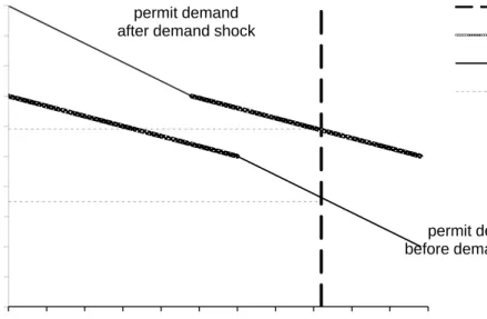
Figure 3. Cost Decrease Shifts Low User Demand (Thin Line) Up by $5, while High User Demand (Thick Line) Is Unchanged

The uniform cost distributions can be used to derive demand functions that would approximate the actual demands resulting from the random cost draws. For high emitters, the cost distribution on the range from $1 to $5 results in values that are distributed from $7, calculated as ($15 – $1)/2, to $5, calculated analogously. Thus demand is 0 at a permit price of $7, and all 60 permits that could be used by high emitters would be demanded at a price of $5. The aggregate demand function that results is QH = 210 – 30P over a price range from [$5, $7], where P is the permit price. Similarly, it is straightforward to show that the cost reduction from [$10, $13] to [$5, $8] for low users will shift their aggregate demand for permits from QL = 80 – 16P over the range from [$2, $5] to a demand of QL = 160 – 16P over the range from [$7, $10]. Recall that the range of permit values for high users is [$5, $7], which is in between the before and after value ranges for low users, so the increase in permit values for low users moves their values from the bottom-right segment of the combined permit market demand to the upper-left

$0 $1 $2 $3 $4 $5 $6 $7 $8 $9 $10 0 10 20 30 40 50 60 70 80 90 100 110 permit demand after demand shock

permit quantity

permit demand before demand shock

auction supply high user demand low user demand equilibrium

Resources for the Future Burtraw et al.

segment, as shown in Figure 3. Note that the Walrasian price prediction increases from about $3.50 for the first three auctions to about $6.00 for the final three auctions.

We ran 6 separate 12-person sessions for each of the six auction formats, for a total of 36 sessions and 432 subjects. As shown in Table 2, there were two sealed-bid auction formats, two continuous formats with fixed time intervals during which bids could be adjusted continuously, and two multiround formats with uniform prices being determined by a “clock” process that adjusts the price in response to excess demand. The random cost draws were balanced across auction treatments in the sense that the same sets of cost draws were used in all treatments.

Table 2. Auction Formats

Timing Pricing

Within-auction information release

Sealed-bid Discriminatory None

Sealed-bid Uniform price None

Continuous Discriminatory Provisional winners

Continuous Uniform price Provisional winners

Multiround clock Uniform clock price None

Multiround clock Uniform clock price Excess demand

In the sealed-bid auctions, bidders submit individual bids for different permits. The bids were ranked from high to low, with the highest 82 bids being accepted. In the discriminatory price auctions, winners “pay as bid,” whereas in the uniform price auction, winners pay the dollar amount of the highest rejected bid, which serves as a market-clearing price. In the

continuous auction formats, bids could be submitted at any time during the five-minute bidding period, with the highest 82 bids at any given time being listed as “conditionally winning.” Bidders could see only their own submitted bids during the auction, with provisionally winning bids shown in green and provisionally losing bids shown in red.11

When the time expired, the highest 82 bids at that moment would be accepted, with prices paid determined as in the sealed-bid auctions, using either a discriminatory (pay as sealed-bid) or a uniform (highest rejected sealed-bid) format.

11

Providing information about others’ bids might enhance price discovery, but revealing information about particular bids during the auction could facilitate collusion. Indeed, this is the reason that RGGI publishes purchase information—the clearing price, the distribution of purchase quantities, and aggregate purchase quantities by user category (compliance entity or broker)—in summary form only ex post. An interesting direction for future research would be to explore the nature of any trade-offs between the value of contemporaneous bid information and any unintended side effects on coordinated bidding.

The clock auctions were multiround auctions in which bidders submitted quantities that they would be willing to purchase at an announced price. Bidding started at the reserve price, and if demand exceeded supply, the price would rise for the next round, like the tick of a clock. An activity rule prevented bidders from increasing their own demand quantities after they had been reduced. The clock would stop when the aggregate quantity demanded was less than or equal to the auction supply.12 As noted above, the two versions of the clock auction differed in terms of whether total demand for permits was announced at the end of each round of bidding. To

maintain comparability across formats, all auctions had a reserve price of $2.50, and the possible bid increments in the single-round auctions corresponded to the clock tick increments.

All subjects were University of Virginia students. Each laboratory session lasted about an hour, including time for instructions. Participants were paid in cash at the end of the session; they received an initial payment of $6 and a payment of 30 cents for each experiment dollar. Earnings from the six auctions ranged from $15 to $45. The experiments were run using the web-based Emissions Permits program that is publicly available on the Auctions menu on the Veconlab site (http://veconlab.econ.virninia.edu/admin.php). A copy of the instructions is provided in

Appendix A.

III. Results

For a given set of random cost draws, it is straightforward to calculate the permit values for each of the 12 bidders in a session. These values can be ranked from high to low to form a demand function for permits, and the intersection with the vertical auction supply of 82 provides a Walrasian price prediction. The averages of the price predictions for all six auctions in

sequence are shown in Figure 4 as the dotted line. Notice that the average Walrasian price prediction jumps from about $3.50 in the third auction to about $6.00 in the fourth, as a result of the reduced costs for low emitters.

12

The experiments implemented a “roll-back” procedure used in the Virginia NOx auction for dealing with the

possibility of excess supply (unsold permits) in the final round. In that case, the clock price would be lowered to the level for the previous round only if that would raise auction revenue. In the event of such a roll-back, the bidders who offered to pay the higher price would receive their full quantity bids (at the lower price), and the remaining allowances would be allocated to bidders who had demanded additional units at the lower price, in a priority determined by the time order in which bids had been received. This time priority was used in the Virginia NOx

Resources for the Future Burtraw et al.

Figure 4. Average Prices Paid for Sealed-Bid Uniform Price Auction and Clock with (“Open”) and without Announced Excess Demand Information Each Round

Figure 4 permits a price comparison for the two versions of the English clock auction, the “open clock” with ex post price information (thick solid line) and the clock with no excess demand information (thick line with dashes and dots). These lines are averages over all six sessions for each treatment, but their proximity to each other suggests our first result, that in this context there is no significant difference between the two versions of the clock auction

(supporting statistical tests will be discussed below). It is not surprising that a multiround auction like the clock will pick up the demand shift, since demand is revealed as the clock price is raised. The observation that final clock prices are always below the Walrasian predictions may be due to tacit collusion, as bidders realize that if they reduce demand, they may stop the clock, lowering the prices for the permits that they do purchase. Also, notice that the downward deviations are somewhat larger for the final three auctions, and in this sense, the clock auctions do not fully track the magnitude of the change in Walrasian price predictions.

For comparison, Figure 4 also shows price averages for the single-round (sealed-bid) uniform price auctions, which tracked the demand shift similarly. As with the clock auctions,

$0.00 $0.50 $1.00 $1.50 $2.00 $2.50 $3.00 $3.50 $4.00 $4.50 $5.00 $5.50 $6.00 $6.50 1 2 3 4 5 6 Auction Price Walrasian Prediction Clock Open Clock Sealed Bid Uniform

that subjects tended to bid low on some units in an effort to reduce the clearing price (highest rejected bid). The reason that prices in the uniform price auctions tended to track the demand shift was that people were bidding near value on some of their permits (those with high use values), which is generally a profitable strategy whether others’ values have changed or not. When bids are tracking values, then a shift in demand caused by increases in the willingness to pay for permits for half of the bidders will also raise the market-clearing uniform price. As shown below, the differences between the two types of clock auctions and the sealed-bid uniform price auctions are not generally significant.

Although none of the auction formats shown in Figure 4 fully capture the high price predictions following the demand shift, one might wonder whether all auctions with this many bidders are equally good. This is clearly not the case, as indicated by the price sequences for discriminatory auctions shown in Figure 5. The discriminatory (sealed-bid, single-round) format did exhibit low average deviations from the Walrasian predictions, but this format did not pick up the shift in demand very well (the thick gray line connecting the average prices paid is too flat). Note that these average prices were biased upward in the first three auctions and downward after the demand shift. The upward initial bias is consistent with a tendency for auction revenues to be relatively high early in a sequence of discriminatory auctions, but this difference tends to diminish over time as bidders adjust bids downward in an attempt to be just above the threshold of the highest rejected bid.13

13

See Shobe et al. (forthcoming), who report an experiment with stationary supply and demand conditions, but with treatments that implement different degrees of “tightness” of the cap (supply) of permits relative to demand..

Resources for the Future Burtraw et al.

Figure 5. Average Prices Paid for Sealed-Bid Discriminatory Auction and Two Continuous Auction Formats (Discriminatory and Uniform Price)

The continuous discriminatory auction (thick dark line in Figure 5) yielded the worst price tracking of any of the five auction types considered. Subjects were generally bidding below their values in the early minutes of these auctions, often near the reserve price level. Some bidders did not even turn in bids in the first three or four minutes. Thus the remaining bidders would see all of their bids displayed as being provisionally accepted, even at low bid levels. Then “sniping” in the final 30 seconds of the auction would raise the cutoff prices, and bidders would scramble to leapfrog their bids upward once or twice if they had time. The resulting prices did not increase to the predicted levels, especially after the demand shift.

The poor price-tracking performance of the continuous discriminatory auction was a bit of a surprise, since we decided to include this format in the experiment after hearing about it from a representative of an auction software vendor. This format had been used for the

procurement of energy by state agencies via “reverse auctions,” in which the low bid (proposed

$0.00 $0.50 $1.00 $1.50 $2.00 $2.50 $3.00 $3.50 $4.00 $4.50 $5.00 $5.50 $6.00 $6.50 1 2 3 4 5 6 Auction Price Walrasian Prediction Sealed Bid Discriminatory Continuous Discriminatory Continuous Uniform

payment to bidder) wins.14 This format recommendation, however, was derived from experience in a different context, a reverse auction for a single procurement contract instead of a normal (high bids win) auction for multiple prizes (blocks of emissions permits). As mentioned in the introduction, a major advantage of an experimental approach is that alternative sets of auction rules can be compared in the same context, and in a setting that more closely matches the situation where the auction will be implemented.

As with the continuous discriminatory auctions, bidders in the continuous uniform

auctions could view the status of their bids (provisionally winning or not) and could increase (but not decrease) their bids at any time prior to the end of the auction. The result of continuous bidding was again a widespread attempt to collude tacitly by bidding at the reserve price on some permits early in the auction, with some bidders not bidding at all until the final seconds. But the uniform price property allowed the bidders the opportunity to bid aggressively for their most valuable permits, to ensure some high-value purchases at a price determined by the highest rejected bid. This demand revelation behavior for high-value units (likely to be purchased) caused the continuous uniform format to outperform the discriminatory auctions at revealing the

magnitude of the predicted price increase after the third auction in each sequence, but levels of average purchase prices were uniformly too low as a result of signaling and bidding at the reserve price until the final seconds, at which time “sniping” was pervasive.

Table 3. Percentage Price Deviations from Walrasian Predictions by Session, before and after Demand Shift

Average price deviations Rounds 1–3

Average price deviations Rounds 4–6

Sealed-bid, discriminatory +26, +8, +20, +2, +24, 0 –8, –23, –15, –25, –10, –33 Sealed-bid, uniform price –16, –14, –21, –7, –13, –11 –10, –7, –29, –14, –9, –18 Continuous, discriminatory –3, –2, –4, –4, –13, –10 –35, –33, –31, –37, –42, –32 Continuous, uniform price –9, –2, –4, –16, –9, +5 –19, –21, –10, –17, –18, –31 Clock (demand hidden) –18, –6, –13, –16, –11, –13 –7, –13, –9, –17, –17, –16 Clock (demand revealed) –11, –11, –14, –4, –6, –11 –19, –4, –19, –7, –14, –21

14

Resources for the Future Burtraw et al.

Table 3 shows the average prices expressed as percentage deviations from the Walrasian predictions for each of the six sessions in a given treatment. These average deviations are shown separately in the table for rounds 1–3 before the demand shift and for rounds 4–6 after the shift. A positive number in the table indicates that the average price for those rounds tends to be above the Walrasian predictions, as is the case for the sealed-bid discriminatory auction. Note that average price deviations are roughly comparable for all auctions with uniform clearing prices, sealed-bid, continuous, and clock, with and without the revelation of excess demand information.

The pairwise differences in the deviations of the clearing prices of each auction format from the Walrasian price are evaluated using the nonparametric Mann-Whitney Wilcoxon test statistic, and the results are reported in Table 4 (these are two-tailed tests). The asterisk indicates where the hypothesis that each pair yields identical price deviations from Walrasian price is rejected with 95 percent confidence. In other words, an asterisk indicates where the two auction formats being compared are yielding different outcomes. The first part of the table compares auction formats for the first three auctions, where the sealed bid discriminatory format is distinguished from all other auction types in the sense that it has significantly higher prices. In addition, the continuous discriminatory auction is distinguished from the sealed-bid uniform and clock auction (demand hidden) formats. Several other comparisons also had fairly low p-values, indicating near statistical significance in rejecting the hypothesis.

Table 4. Comparison of Percentage Deviations from Walrasian Price First 3 auctions Last 3 auctions

Auction format pairing

Test

statistic p-value

Test

statistic p-value

Sealed-bid uniform, continuous uniform 27 0.06 47 0.24

Sealed-bid uniform, sealed-bid discriminatory 21 0.00* 44 0.48

Sealed-bid uniform, continuous discriminatory 23 0.01* 57 0.00*

Sealed-bid uniform, clock (demand hidden) 37.5 0.85 38 0.94

Sealed-bid uniform, clock (demand revealed) 27.5 0.07 41 0.82

Continuous uniform, sealed-bid discriminatory 23 0.01* 38 0.94

Continuous uniform, continuous discriminatory 33 0.39 56 0.00*

Continuous uniform, clock (demand hidden) 51 0.06 26.5 0.05*

Continuous uniform, clock (demand revealed) 46 0.31 32 0.31

Sealed-bid discriminatory, continuous discriminatory 54 0.02* 54 0.02*

Sealed-bid discriminatory, clock (demand hidden) 57 0.00* 33 0.39

Sealed-bid discriminatory, clock (demand revealed) 57 0.00* 32 0.31

Continuous discriminatory, clock (demand hidden) 55 0.01* 21 0.00*

Continuous discriminatory, clock (demand revealed) 51 0.06 21 0.00*

For the final three auctions after the demand shift, there was more separation, with several auction types clearly distinguished and several nearly identical. Table 4 confirms the impression given in Figures 4 and 5, with continuous discriminatory always producing a different average price compared with the other formats. The only other distinction with statistical significance is the comparison of the deviations from the Walrasian price of the continuous uniform and the clock (with demand hidden) formats, which had lower absolute deviations. There were no other comparisons with very low p-values for the last three auctions.

Up to this point, the discussion has focused on a comparison of auction formats in terms of how close prices are to Walrasian predictions, either before or after the demand shift. The main focus of this research is on how well each auction format tracks changes in the underlying structure of the market, and one way this issue could be addressed is by comparing price

deviations from predictions before and after the demand shock for a given auction format. If the deviations tend to be the same before and after, then the change in prices is in line with the predicted change, even if absolute price levels are a little biased both before and after. Table 5 reports the average price deviations of each auction format for the first three auctions compared with the last three auctions for the same auction format. The hypothesis being tested using the Mann-Whitney Wilcoxon test statistic is that the deviation from the Walrasian price is the same for the first three auctions as for last three auctions. The asterisk indicates where the hypothesis that the each pair yields identical price deviations from the Walrasian price is rejected with 95 percent confidence. The hypothesis is rejected for the continuous uniform, sealed-bid

discriminatory, and continuous discriminatory, indicating these auction formats failed to track the cost-induced change in the demand for allowances.

Table 5. Comparison of Deviations from Walrasian Price for Each Auction Format, before and after Demand Shock

Auction format Test statistic p-value

Sealed-bid uniform 6.00 0.44

Continuous uniform 0.00 0.03*

Sealed-bid discriminatory 0.00 0.03*

Continuous discriminatory 0.00 0.03*

Clock (demand hidden) 9.00 0.84

Clock (demand revealed) 3.00 0.16

IV. Conclusion

Resources for the Future Burtraw et al.

conditions and regulatory risks. The evidence for price tracking is somewhat indirect, however, and comparisons across auction formats are further complicated by differences in underlying regulatory conditions. In particular, it would be very difficult to establish a performance benchmark by estimating Walrasian price predictions for the various allowance markets.

Laboratory experiments have been used to compare alternative auction formats, taking advantage of the ability to control extraneous factors by framing comparisons in comparable settings, with identical sequences of Walrasian price predictions. Replication with multiple sessions involving different groups of financially motivated participants allows us to separate general tendencies from the noise associated with particular combinations of individual behavior patterns. The experiments can be structured to provide stress tests that provide a sharper focus on potential strengths and weaknesses of alternative auction formats.

In previous work providing guidance for the Regional Greenhouse Gas Initiative

(Burtraw et al., 2009; Holt et al. 2007), we have shown that the effects of collusion can be more pronounced in multiround clock auctions for emissions permits, which is consistent with other experimental results. In our experiments, the effects of successful collusion are apparent in cases where the clock stops at the reserve price in the first round, or when trading in subsequent spot markets is at prices that are way above the final clock price in the preceding auction.15 Our recommendation for the design of RGGI auctions was to use a simple uniform price auction, since it was found to be transparent, simple, and resilient to collusion. In a subsequent study, we compared the uniform price auction with some alternatives in a particularly stressful

environment in which the number of permits being auctioned was only slightly below the number that would be demanded at a zero price (Shobe et al., 2009). In fact, the uniform price, discriminatory, and clock auctions performed equally well after an initial adjustment period in this “loose cap” environment, although revenue was higher with the discriminatory format in the initial auctions.

In this paper, we report another stress test, involving a large, unanticipated shift in the demand for permits. This demand-shift experiment yields three main conclusions: (1) uniform price auctions (clock and sealed-bid uniform price, and continuous uniform) generate changes in purchase prices that are reasonably close to the Walrasian predictions. (2) There is some

evidence that tacit collusion causes prices to be too low relative to predictions in most cases, and

15

This result was replicated in the same environment and extended to markets with speculators by Naegelen et al. (2009). Goeree et al. (2006) also report high levels of tacit collusion in a clock auction, in a different context.

such tacit collusion is most successful for the multiround and continuous formats (clock with and without information about excess demand, continuous discriminatory, and continuous uniform), where signaling was possible to some extent, especially in the continuous auctions. (3) The worst price tracking occurred with the continuous discriminatory auction, where the combined effects of signaling and sniping all but hid the effects of the unanticipated demand shift. Overall, the clock and sealed-bid uniform price auctions performed best in this demand-shift environment.

Appendix A. Instructions (Uniform Price)

Permits: This is an auction in which you have the role of a producer that must obtain "permits" in order to produce a product.

Production: Producers will be given a number of capacity units. Think of each capacity unit as a plant that can produce one unit of output. You will be told the cost of operating the capacity unit, and the unit profit will be the price of the product minus the cost for that unit.

Permit Prices: Producers may buy permits at auction to operate your capacity units, and the prices paid for these permits will be added to your costs. There are 12 participants who will be bidding for permits.

Permit Requirements: You will be told the number of permits needed to operate each of your capacity units. Some of you will be high users who require more permits to operate than others, and others will be low-users, as explained subsequently.

Output Price: In addition, you will know the price at which the output produced by a capacity unit can be sold. Continue.

Example: Suppose you have one capacity unit with a cost of $1.00 and the output from this unit can be sold for a known price of $5.00. Thus the earnings would be $4.00 on this

capacity unit in the absence of the need to obtain permits. A regulation requires that this capacity unit must have one or more permits to operate.

Permit Auction: Permits will be sold at auction. In this example, suppose that you need 1 permit to operate a capacity unit; if you can buy a permit for less than $4.00, you can earn the difference. If you do not have a permit, the capacity unit cannot be operated and your earnings are $0.00 for the unit.

Resources for the Future Burtraw et al.

Types of Firms: In total, there are 6 firms in this market who require 1 permit to operate each capacity unit. In addition, there are 6 firms in this market who require 2 permits to operate each capacity unit. Your role is that of a *** .

Random Costs: Costs differ from one person to another, and new random costs are determined for each person at the start of each new auction. Continue

You will have ** units of capacity as shown by the rows in the table below.

Each unit produces a product that is sold for $15.00 (2nd column).

Your units are listed in order of increasing cost (3rd column).

One or more permits are needed to operate each capacity unit (4th column).

The value of a permit is the difference between the output price and the unit cost, divided by the required number of permits (5th column).

Permits are indistinguishable, so you will be using the ones you obtain on the capacity units with low costs (and high values) at the top of the table.

Remember that your earnings will be determined by differences between the values for permits used and what you pay for the permits.

Capacity Unit Output Price Unit Cost Permits Required Permit Value 1 $15.00 $*.** * $0.00 2 $15.00 $*.** * $0.00 3 $15.00 $*.** * $0.00 4 $15.00 $*.** * $0.00 5 $15.00 $*.** * $0.00 6 $15.00 $*.** * $0.00 7 $15.00 $*.** * $0.00 8 $15.00 $*.** * $0.00

Permit Auction: A total of 82 permits will be sold in a single-round auction in which bids must be above a reserve price, $2.50.

Bidding: You begin by indicating a bid for each permit you desire; you may bid different amounts for different permits or groups of permits.

Winner Determination: All bids are collected and ranked, and the 82 highest bids are accepted, but the winning bidders only have to pay the amount of the highest rejected bid (of rank 82 + 1). There is only one round of bidding, and ties are decided by a random device.

Uniform Price: Note that all permits end up being sold at the same price, which will generally be lower than your bids. Continue

Bidder Activity Limits: The auction rules and financial pre-qualifications have determined a maximum number of permits that can be bid for in the auction by each person. Your activity limit is ** permits.

Series of Permit Auctions: There will be a number of auctions, and you can bid for any number of permits up to your activity limit in each auction.

Production Decision: After you know how many permits you have to work with, you will decide which capacity units to operate, i.e. how many permits to use.

Preview: The next page will explain how the spot market works. Continue.

There will be a series of permit auctions in which bidders will submit bids for permits, which will be ranked from high to low. The 82 permits will be sold to the highest bidders at a single, uniform price that is the amount of the highest rejected bid, so all winning bidders will pay the same price.

Note: You must pay the highest rejected bid if your bids are above that level, so you may lose money if you bid for one or more permits at prices that exceed your values for those permits. On the other hand, you may not obtain the permits needed to make money if you bid too low.

After each permit auction, you can use the permits acquired to produce units of a product sold at $15.00 per unit.

Permits are identical, but they must be used when they are acquired; they cannot be "banked" from one production period (following each auction) to the next.

The number of auctions will not be announced in advance.

Your earnings for each auction = output price(s) received - cost(s) of capacity units used - price(s) paid for permits. These earnings will be summed for all auctions to determine your cumulative earnings.

Resources for the Future Burtraw et al.

Special Earnings Announcement: Your cash earnings will be 30% of your total earnings at the end of the experiment.

References

Burtraw, D., J. Goeree, C.A. Holt, E. Myers, K. Palmer, and W. Shobe (2009) “Collusion in Auctions for Emissions Permits: An Experimental Analysis,” Journal of Policy Analysis and Management 28(4), 672–691.

Davis, D.D., and C.A. Holt (1993) Experimental Economics, Princeton, NJ: Princeton University Press.

Ellerman, A.D., P.L. Joskow, R. Schmalensee, J. Montero, and E. Bailey (2000) Markets for Clean Air: The U.S. Acid Rain Program, New York: Cambridge University Press. Goeree, J.K., T. Offerman, and R. Sloof (2006) “Demand Reduction and Preemptive Bidding in

Multi-Unit License Auctions,” Discussion Paper, CalTech.

Holt, C., W. Shobe, D. Burtraw, K. Palmer, and J.K. Goeree (2007) “Auction Design for Selling CO2 Emission Allowances under the Regional Greenhouse Gas Initiative,” RGGI

Reports, Albany: New York State Energy Research and Development Authority. Porter, D., S. Rassenti, W. Shobe, V. Smith, and A. Winn (2009) “The Design, Testing, and

Implementation of Virginia's NOx Allowance Auction,” Journal of Economic Behavior and Organization 69(2): 190–200.

Naegelen, F., M. Mougeot, B. Pelloux, and J.-L. Rullière (2009) “Breaking Collusion with Speculation: An Experiment on CO2 Permits Auctions,” presented at the Economic Science Association Meetings, Tucson, AZ.

Shobe, W., K. Palmer, E. Myers, C.A. Holt, J. Goeree, and D. Burtraw (forthcoming) “An Experimental Analysis of Auctioning Emissions Allowances under a Loose Cap,”