6-2019
A Cyberinfrastructure for Big Data Transportation Engineering
A Cyberinfrastructure for Big Data Transportation Engineering
Md Johirul IslamIowa State University, mislam@iastate.edu
Anuj Sharma
Iowa State University, anujs@iastate.edu
Hridesh Rajan
Iowa State University, hridesh@iastate.edu
Follow this and additional works at: https://lib.dr.iastate.edu/cs_pubs
Part of the Databases and Information Systems Commons, and the Transportation Engineering Commons
The complete bibliographic information for this item can be found at https://lib.dr.iastate.edu/
cs_pubs/20. For information on how to cite this item, please visit http://lib.dr.iastate.edu/ howtocite.html.
This Article is brought to you for free and open access by the Computer Science at Iowa State University Digital Repository. It has been accepted for inclusion in Computer Science Publications by an authorized administrator of Iowa State University Digital Repository. For more information, please contact digirep@iastate.edu.
Abstract Abstract
Big data-driven transportation engineering has the potential to improve utilization of road infrastructure, decrease traffic fatalities, improve fuel consumption, and decrease construction worker injuries, among others. Despite these benefits, research on big data-driven transportation engineering is difficult today due to the computational expertise required to get started. This work proposes BoaT, a transportation-specific programming language, and its big data infrastructure that is aimed at decreasing this barrier to entry. Our evaluation, that uses over two dozen research questions from six categories, shows that research is easier to realize as a BoaT computer program, an order of magnitude faster when this program is run, and exhibits 12–14× decrease in storage requirements.
Keywords Keywords
Big Data, Domain-specific-language, Cyberinfrastructure
Disciplines Disciplines
Civil and Environmental Engineering | Computer Sciences | Databases and Information Systems | Transportation Engineering
Comments Comments
This is a pre-print of an article published as Islam, Md Johirul, Anuj Sharma, and Hridesh Rajan. "A Cyberinfrastructure for Big Data Transportation Engineering." Journal of Big Data Analytics in
Transportation 1, no. 1 (2019): 83-94. The final authenticated version is available online at DOI: 10.1007/
s42421-019-00006-8. Posted with permission.
Md Johirul Islam mislam@iastate.edu Anuj Sharma anujs@iastate.edu Hridesh Rajan hridesh@iastate.edu
Word Count: 4217 words + 13 figure(s) x 250 + 0 table(s) x 250 = 7467 words
Submission Date: May 2, 2018
ABSTRACT
Big Data-driven transportation engineering has the potential to improve utilization of road in-frastructure, decrease traffic fatalities, improve fuel consumption, decrease construction worker injuries, among others. Despite these benefits, research on Big Data-driven transportation engi-neering is difficult today due to computational expertise required to get started. This work pro-poses BoaT, a transportation-specific programming language, and its Big Data infrastructure that is aimed at decreasing this barrier to entry. Our evaluation that uses over two dozen research questions from six categories show that research is easier to realize as a BoaT computer program, an order of magnitude faster when this program is run, and exhibits 12-14x decrease in storage requirements.
INTRODUCTION
The potential and challenges of leveraging Big Data in transportation has long been recognized (1–
14). For example, researchers have shown that Big Data-driven transportation engineering can help
reduce congestions, fatalities and make building transportation applications easier (4, 5, 13). The
availability of open transportation data that is accessible e.g. on the web under a permissive license, has the potential to further accelerate the impact of Big Data-driven transportation engineering.
Despite this incredible potential, harnessing Big Data in transportation for research remains difficult. In order to utilize Big Data, expertise is needed along each of the five steps of a typical data pipeline namely data acquisition; information extraction and cleaning; data integration,
ag-gregation, and representation; modeling and analysis; and interpretation (1). First three steps are
further complicated by the heterogeneity of data from multiple sources (3), e.g. speed sensors,
weather station, national highway authority. A scientist must understand the peculiarities of the data sources to develop a data acquisition mechanism, clean data coming from multiple sources, and integrate data from multiple sources. Modeling and analysis are complicated by the volume of the data. For example, a dataset of speed measurements from a commercial provider for Iowa for a single day can be in multiple GBs, exceeding the limits of a single machine. Analyses that aim to compute trends over multiple years can easily require storing, and computing over, tens of TBs of just speed sensor data.
A possible solution could be to use the Big data technologies like Hadoop, Apache Spark running over a distributed cluster. Using a distributed cluster with an adequate number of nodes problems related to the storage and time of computation can be addressed. But these Big Data technologies are not so easy to use. Getting started requires technical expertise to set up the infrastructure, efficient design of data schema, data acquisition strategy from multiple sources, high level of programming skills, adequate knowledge of distributed computing models and a lot more efficiency in writing distributed computer programs which is significantly different than writing a sequential computer program in Matlab, C or Java. The analysis of Big Data in transportation is almost an elite job due to these barriers. The research groups interested in Big Data-driven transportation engineering have to hire technically skilled people or train their own staff members to use these highly sophisticated technologies. Both approaches incur additional costs.
This work describes a transportation-specific Big Data programming language and its
in-frastructure that is aimed at solving these problems. We call this language BoaT (Boa(15) for
Transportation). The BoaT infrastructure provides build-in transportation data schemas and con-verters from existing data sources. A notable advantage of BoaT’s data schema is a significant re-duction in storage requirements. A transportation researcher or engineer can express their queries as simple sequential looking BoaT programs that is another advantage of the approach. The BoaT infrastructure automatically converts a BoaT program to a distributed executable code without sac-rificing correctness in the conversion process. This also often results in an order of magnitude improvement in performance that is the third advantage of our approach. The BoaT infrastructure provides build-in transportation data schemas and converters from existing data sources. The four notable advantages of BoaT are : a.) significant reduction in storage requirement by using specially designed data schema, b.) A transportation researcher or engineer can express their queries as sim-ple sequential looking BoaT programs, c.) auto conversion of sequential programs to a parallelly executable programs without sacrificing correctness in the conversion process, d.) The number of lines of code significantly reduces thus reducing the debugging time for the program. Owing to
these advantages, even users that are not experts in distributed computing can write these BoaT programs that lower the aforementioned barrier to entry.
The remainder of this article describes the BoaT approach and explores its advantages. First, in the next section, we motivate the approach via a small example. Next, we compare and contrast this work with related ideas. Then, we describe the salient technical aspects of the tech-nique. Next, we evaluate the usability, and scalability of the technique, show some example use cases that we have realized, and highlight benefits of our storage strategy. Finally, we conclude. MOTIVATION
Transportation agencies collect a lot of data to make critical data driven decision for Intelligent Transportation System (ITS). There has been a lot of initiative to make data available for
re-searchers to spur innovation (16). But the analysis of this ultra large-scale data is a difficult task
given the technology needed to analyze the data is still a luxury (17). These data come from
mul-tiple sources with a lot of varieties, velocities, and volumes. Given the availability of a variety of sources of data technically skilled people also often face challenges due to the kinds of input, data
access patterns, type of parallelism, etc. Kambatla et al. (18). The need to write complex programs
can be a barrier for domain researchers to take the advantage of this large-scale data. To illus-trate the challenges, consider a sample question “Which counties have highest and lowest average temperature in a day?” A query like this is simple when the data is already provided by county but in case you have data for every 5 minute for every square mile of Iowa for last 10 years. The query becomes hard to solve in Matlab or even R and could potentially run for a long time in Java Answering this question in Java would require knowledge of (at a minimum): reading the weather data from the data provider service, finding the locations and county information of different grids from some other APIs, additional filtering code, controller logic, etc. Writing such a program in Java, for example, would take upwards of 100 lines of code and require knowledge of at least 2 complex libraries and 2 complex data structures. A heavily elided example of such a program is shown in Figure 1, left column.
This program assumes that the user has manually downloaded the required weather data, preprocessed the data and written to a CSV file. It then processes the data and collects weather information in different grids at different times of the day. Next, the county information of each grid is found from another API. Finally, the data is stored in some data structures for further computation. The presented program is sequential and will not scale as the data size grows. One could write a parallel computation program which would be even more complex.
We propose a domain-specific programming language called BoaT to solve these problems. We intend to lower the barrier to entry and enable the analysis of ultra-large-scale transportation data for answering more critical data-intensive research challenges. The main features of Boa for
transportation data analysis originated from (15, 19–21). To this, we add builtin transportation
specific data types and functions for analysis of large-scale transportation data, schema, and in-frastructure to preprocess data automatically and store efficiently. The main components come as an integrated framework that provides a domain specific language for transportation data analysis, a data processing unit, and a storage strategy.
RELATED WORK
Due to the rapid growth of data-driven Intelligent transportation system (ITS) El Faouzi et al.
ultra-large-J a v a 1 ... // imports 8 public class CountiesMaxAvgTmpc { 9 public static void main(String[] args){ 10 ... // File operation 11 PriorityQueue<CountyTemp> maxheap , minheap; 12 ... // data processing 65 private String buildHeaps( /* input heaps * / ) { 66 ... // Populate the heaps with Objects 67 } 72 ... // Iterating over the Map to find average temperature of each county 73 for (Map.Entry<String, List<Double>> entry : map .entrySet()) { 74 String county = entry.getKey(); 75 List<Double> countyTemps = entry.getValue() ; 76 for ( double temp : countyTemps){ 77 ... // Iterating over the county temp for avg 78 } 89 // Getting County name from another data file given the grid id 90 public static String getCounty( int gridid) { 91 ... // Code to find county from grid 92 } 93 // Internal class to hold county data 94 private static class CountyTemp { 95 ... // County variables 96 public CountyTemp(String countyName, double temperature) { 97 ... // Constructor 98 } 99 ... // codes to manage county data 100 } 101 public static String getCounty( int gridid) { 102 ... // Getting County from a grid id from API 103 String county = getCountNameFromAPI(gridid) ; BoaT 1 p: County = input ; 2 max: output maximum (1) of string weight float; 3 min: output minimum (1) of string weight float; 4 count := 0; 5 sum := 0.0; 6 visit (p, visitor { 7 before n: Grid -> { 8 weatherRoot := getweather(n, " 5-11-2017 " ); 9 foreach (s : int ; def (weatherRoot.weather[s])) { 10 sum = sum + weatherRoot.weather[s].tmpc; 11 count++; 12 } 13 } 14 }); 15 max << p.countyName weight sum /count; 16 min << p.countyName weight sum /count; P erf ormance FIGURE 1 : Programs for answering "Which counties ha v e highest and lo west av erage temperature in a day?" and the performa nce with the size of data
scale data is becoming more important today than any time before. Though a lot of works are done on data-driven smart city design and Big data analysis, trying to tackle the challenges of transportation big data from the domain-specific language perspective is few. In other domains, a lot of advantages are being taken from Big data using Domain Specific programming languages.
For example, Dyer et al. (15) used the early version of Boa to analyze ultra-large-scale software
repository data (data from repositories like GitHub). However, Dyer et al.’s work is limited to
software repositories whereas BoaT built on top of Boa is provides the support of transportation data analysis at ultra-large scale, transportation domain types and an infrastructure of efficient data storage from a variety of transportation data sources.
There has been some efforts to support domain types and computation in transportation
in an integrated modeling tool called UrbanSim Borning et al. (24), Borning et al. (25), Waddell
et al. (26). UrbanSim is an integrated modeling environment that provides a modeling language
which provides access to urban data for finding models to coordinate transportation and land usage
Waddell et al. (26). While UrbanSim focuses on simulation, BoaT is for analyzing gathered data.
Furthermore, supporting analysis of large-scale data has not been the focus of UrbanSim, whereas
BoaT focuses on providing scalable support for data analysis. Simmhan et al. (27) provides a
cloud-based software platform for data analytics in Smart Grids, whereas BoaT is focussed on
transportation data. Du et al. (28)’s City Traffic Data-as-a-Service (CTDaaS) uses service-oriented
architecture to provide access to data, but does not focus on the scalable analysis of Big Data. In general, the current approaches using big data analytics are either using costly cloud computation or have custom build design for solving specific problems using open source solution
with on-premise servers. Works such as Yang and Ma (29) and Wang and Li (30) highlight the
challenges of doing Big Data-driven transportation engineering today. For example, Yang and Ma
(29) use HDFS, MLlib, cluster computing to solve their problems, essentially like our
motivat-ing example. Each of these technologies creates its own barrier to entry. There is a need for a framework that would overcome the barrier to use big data analytics, provide a domain specific language, reduce the efforts of data preprocessing and will be available at a mass scale.
BOAT: DESIGN AND IMPLEMENTATION
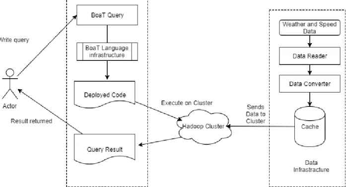
To address the challenges of easy and efficient analysis of big transportation data we propose a transportation-specific programming language and data infrastructure. The language provides simple syntax, domain-specific types and massive abstractions. An overview of the infrastructure is shown in Figure 2.
The user writes the BoaT program and submits it to the BoaT infrastructure, The BoaT program is taken by the infrastructure and converted by a specialized compiler that we have written to produce an executable that can be deployed in a distributed Hadoop cluster. This executable is run automatically on curated data to produce output for the user.
To illustrate, consider the question in Section 3 “Which counties have the highest and the lowest average temperatures in a day?”. A BoaT program to answer this question is shown in Figure 1, right column. Line 1 of the program says that it takes a County as input. So, if there are n counties in the dataset, the statements on lines 4-16 of this program would be automatically run in parallel by the BoaT infrastructure (once for each county). Line 2 and 3 of this program declares
output variables. Thesewrite onlyoutput variables are shared between all parallel tasks created by
the BoaT infrastructure and the infrastructure manages the details of effectively interleaving and maximizing performance. Line 2 says that this output variable will collect values written to it and
FIGURE 2: An Overview of BoaT: shows workflow of a BoaT user and BoaT infrastructure
compute the maximum of those values. This is calledaggregationin BoaT and several other kinds
of aggregation algorithms are supported as shown in Figure 4. Line 15 shows an example of writing to that output variable. Lines 4-16 are run sequentially for each county. They look into each grid of the county (lines 6,7,14) to find temperature data of the grid while maintaining a running sum and frequency to compute average on lines 15-16. While the details of this program are important also, astute readers would have surely observed that writing this program needed no knowledge of how the data is accessed, what is the schema of the data, how to parallelize the program. No parallelization and synchronization code is needed. The BoaT program produces result running in a Hadoop cluster. So the program scales well saving hours of execution time.
As the program runs on a cluster it outperforms the Java program (sequential) as the input data size grows. A comparison is shown in Figure 1 on the lower right corner. The BoaT program provides output almost 20.4 times faster only on one-day weather data of Iowa (10GB). To achieve these goals we have solved following problems.
• Providing transportation domain types and functions;
• designing the schema for efficient storage strategy and parallelization; and • providing an effective solution to data fusion.
Language Design
The language BoaT is the extended version of work done by Dyer et al. (15). They provide the
syntax and tools to analyze the mining software repository data. We extended their work to provide domain types, functions and computational infrastructure for Big Data-driven transportation engi-neering. We create the schema using Google protocol buffer. Google protocol buffer is an efficient
Dyer et al. (15) data representation format that provides faster memory efficient computation in
Domain Types
Type Attributes Details
countyCode Code of the county
County countyName Name of the county
Grids List of Grid in the county.
ID ID of a grid
Grid Location Spatial location of the grid
WeatherRoot Link to the Weather data for the grid
SpeedRoot Link to the speed data for that grid
SpeedRoot speedRecords List of SpeedRecord
WeatherRoot weatherRecords List of WeatherRecord
detectorcode The code of the detector giving the current record
type Type of the vehicle
SpeedRecord speed Speed of the vehicle
reference Reference speed
time Time of the record
roadname Name of the road of the record
tmpc 2 m above the ground level temperature
wawa Watches, warnings, and advisories issued by the National Weather Service
ptype Type of Precipitation
dwpc Dew point temperature
smps Wind speed
WeatherRecord drct Wind direction
vsby Horizontal visibility from sensors in Km
roadtmpc Pavement surface temperature
srad Solar radiation
snwd Snow fall depth
pcpn Precipitation accumulation
time Time of the reading
FIGURE 3: Domain types for transportation data in BoaT
Aggregator Description
MeanAggreagtor Calculates the average
MaxAggreagtor Finds the maximum value
QuantileAggregator Calculates the quantile. An argument is passed to tell the quantile of interest
MinAggregator Finds the minimum value
TopAggregator Takes an integer argument and returns that number of top elements
StDevAggregator Calculates the standard deviation
FIGURE 4: Aggregators in BoaT
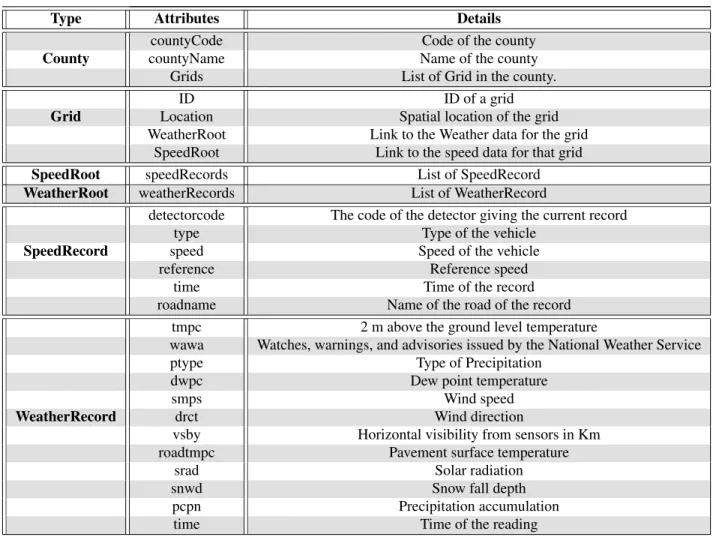
The transportation-specific types in BoaT are shown in Figure 3. As we and others use this infrastructure these types will surely evolve, and the BoaT infrastructure is designed to support such evolution. County is the top level type. This type has attributes that relate to the code of the county, name of the county and a list of grids in the county. A grid is related to a location in a county. For the convenience of computation, the whole Iowa is split into 213840 Grids by Iowa DOT. So we also used Grid as the domain. The Grid has attributes Id, reference to the WeatherRoot
which refers to the weather records in that Grid, reference to SpeedRoot which refers to the Speed records in that Grid. Weather root contains a list of weather records. SpeedRoot contains a list of Speed records. So we can easily go to the speed or weather data of a particular location in a particular Grid under a particular County without searching through all the data in the cluster. SpeedRecord contains the attributes detectorCode, type of detector, average, reference, roadname and time.
The data design has led to two innovations. First to balance query speed, flexibility, and storage capacity. Second to allow future extension via data fusion.
While designing the schema we came to a successful data reduction strategy after multiple trials. Initially, we were using all the data at the top level. That means when we access a row we accessed all the relevant data for that row like weather, speed. Following this strategy, the storage size increased than the raw data. Then we split the data keeping county data at the top level and the relevant weather, speed records at the second level in the same list. We were not getting enough mappers to make a lot of parallelization in the program as the splitting was not possible. And at the same time storage size was almost near the raw data size. Then we made multiple levels of hierarchy in our type system. The top level is the county. The county contains a list of grids (spatial locations), each grid contains two optional fields to point to speed data and weather data. This strategy of data representation gives us benefit in storage as well as in faster computation as only relevant data is accessed. We can store incremental data without regenerating the whole dataset from the beginning. Without this hierarchical schema strategy, all the data need to be merged together creating a merged schema hampering the sustainability, scalability and storage benefit of the system. And the addition of new data would be impossible.
Fusion of multiple data sources in existing big data frameworks is difficult due to size, the necessity of join and parallel queries in the data sources. In BoaT, we addressed this problem in data infrastructure. Any new dataset can be added to the infrastructure easily. For example, we started with speed dataset initially and we were able to answer questions on speed data. The access link to speed data is optional. That means we don’t load the data unless it is necessary. Then we added another optional link to weather dataset. We came up with a successful fusion of data and were able to answer queries that cover both speed and weather dataset without losing any perfor-mance. The queries of category E in Figure 5 are examples of using the fusion of weather and speed dataset. And the performance is not affected by this. This makes our infrastructure sustain-able to any new datasets of interest to be added to the infrastructure. To do that we have to just add an optional link to that new dataset after providing the schema for new dataset. The infrastructure will take care of all other complexities related to data generation, and type generation.
EVALUATION AND RESULTS
This section evaluatesapplicability, scalability, andstorage efficiencyof BoaT and its
infrastruc-ture. By applicability we mean whether a variety of transportation analytics use cases can be pro-grammed using BoaT. By scalability we mean whether the resulting BoaT programs scale when more resources are provided. By storage efficiency we mean whether storage requirements for data are comparable to the raw data, or whether BoaT requires less storage, and if so how much. Applicability
To support our claim of applicability we use BoaT to answer queries on weather and speed data to provide answers to multiple queries from different categories and classes. A small BoaT
pro-LOC R T ime (sec) T ask Classification J a v a BoaT Diff J a v a BoaT Speedup A. T emperatur e Statistics 1. Compute the mean, standard de viation of temperature Central T endenc y 84 10 8.4x 465 22 21.14x 2. Find the top ten counties with highest temperature Rank 90 17 5.29x 470 20 23.50x 3. Find the top ten counties with lo west temperature Rank 85 14 6.07x 489 25 19.56x 4. Find the highest and lo west temperature in dif ferent Counties Rank 70 8 8.75x 485 23 21.09x 5. Find the correlation between Solar radiation and temperature Correlation 65 10 6.50x 460 18 25.56x 6. Find the locations belo w a threshold temperature Anomaly 69 11 6.27x 498 17 29.29x B. W ind Beha vior 1. Compute the mean, standard de viation of wind speed Central T endenc y 97 12 8.083x 2753 48 57.35x 2. Find the top ten locations with higher wind speed Rank 85 9 9.44x 2960 57 51.93x 3. Find the range across of wind dif ferent Counties Rank 65 12 5.42x 2793 45 62.07x 4. Find the correlation between temperature and wind speed Correlation 90 15 6.00x 2743 43 63.79x 5. Find the locations abo v e a threshold weather speed Anomaly 65 10 6.50x 2894 47 61.57x C. Study of pr ecipitation beha vior 1. Compute the mean, Standard de viation, Quantile of Precipitation Central T endenc y 65 17 3.82x 2883 51 56.53x 2. Find the top ten Counties with high precipitation Rank 35 10 3.50x 2945 46 64.02x 3. Find the correlation of temperature with precipitation Correlation 80 9 8.89x 2980 45 66.22x 4. Find the correlation of visibility with precipitation Correlation 80 8 10.00x 2401 53 45.30x 5. Find the locations where precipitation w as abo v e a threshold limit Anomaly 72 6 12.00x 2180 48 45.42x D . Study of Speed 1. Compute the mean, standard de viation of speed at dif ferent locations Central T endenc y 100 17 5.88x 860 31 27.74x 2. Find the top ten counties with higher av erage speed Rank 80 9 8.89x 815 25 32.60x 3. Find the road names with higher av erage Speed? Rank 75 11 6.82x 810 27 30.00x 4. Find the county with maximum and minimum av erage speed Rank 90 8 11.25x 986 35 28.17x E. Effect of weather on speed 1. Find the Correlation between speed and precipitation Correlation 150 13 11.54x 4230 130 32.54x 2. Find the Correlation between Speed and V isibility Correlation 150 13 11.54x 4213 132 31.92x 3. Find which weather parameter is more correlated with speed Correlation 165 17 9.71x 4560 135 33.78x F . Speeding V iolations 1. Find the number of v ehicles running abo v e a speed limit in dif ferent locations Anomaly 80 12 6.67x 980 28 35.00x 2. What is the percentage of v ehicles abo v e reference speed at dif ferent locations? Anomaly 95 15 6.33x 953 23 41.43x 3. Find the number of under speeding v ehicles at dif ferent locations Anomaly 80 12 6.67x 910 27 33.70x FIGURE 5 : Example of BoaT programs to compute dif ferent tasks on transportation data
gram can answer queries that would need a lot of efforts with other general purpose languages, distributed system and data processing. We provide a range of queries in six different categories and four different classes in table shown in Figure 5.
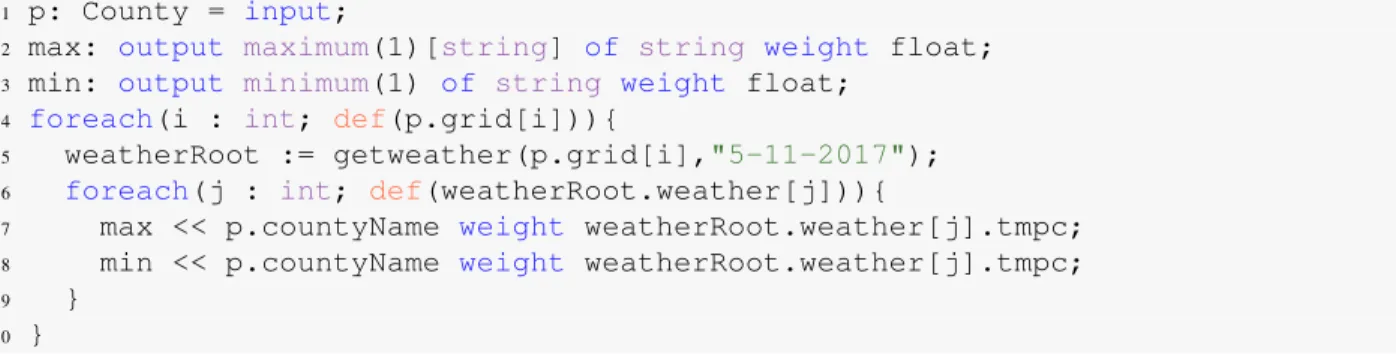
As an example scenario, we consider that a researcher wants to know the maximum and minimum temperature in different counties of a state in the USA in a date in May 2017. To achieve the result in the above scenario we have to write a small program in Figure 6. All the complex technical details of Big Data analytics are abstracted from the user. Lets go through the program to understand what this small program is doing. In Line 1 we are taking the data as input. In our BoaT infrastructure, we currently use county as the top level entry point. In Line 2 and Line 3 we are declaring two output variables. The declaration tells clearly that one variable is going to store the maximum of some floating point numbers having a String i.e. the county name as key and the other variable is going to store the minimum of some floating point numbers. The floating point numbers here are temperature found from the data. In the next line there is a loop to iterate over all the grids of the county and for each county, we assign the temperature at that grid as weight. The program keeps track of the temperature values for each county and at the end returns maximum and minimum temperature at different counties in a day.
1 p: County = input;
2 max: output maximum(1)[string] of string weight float; 3 min: output minimum(1) of string weight float;
4 foreach(i : int; def(p.grid[i])){
5 weatherRoot := getweather(p.grid[i],"5-11-2017"); 6 foreach(j : int; def(weatherRoot.weather[j])){
7 max << p.countyName weight weatherRoot.weather[j].tmpc; 8 min << p.countyName weight weatherRoot.weather[j].tmpc;
9 }
10 }
FIGURE 6: Task A.4: Find the highest and lowest temperature in different counties
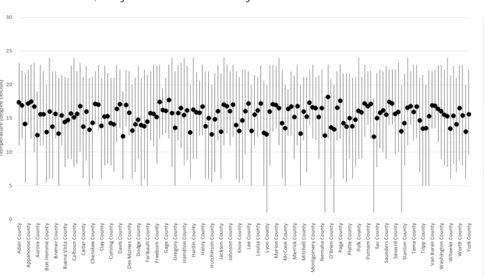
The output of the program is shown in Figure 7. Figure 7 also contains average temperature which is computed from the task A.1.
To go through another example lets take the task D.1. Here we calculate the mean and standard deviation of speed at different locations. The program is given in Figure 8
The program like the program in Figure 6 first declares the output types. The output vari-able for mean uses the MeanAggregator in BoaT and the output varivari-able for standard deviation uses the StDevAggregator. The program iterates through each county one by one and all the grids in that county. While visiting a grid of the county the program gets the speed data at that grid by
us-ing a domain specific functiongetspeed(). The functiongetspeed()has multiple versions
and the version that we are using in this program takes the grid and a date as input and returns the speed data of that grid on that day. Then for each record of the speed data, we aggregate the values in the output. These visits run in different mapper nodes and the aggregation is done in different reducer nodes. Finally, the result is returned to the user.
We use two metrics to evaluate BoaT’s applicability.
• LOC: Line of Code. The total lines needed to write the program • RTime: Runtime of the program
FIGURE 7: Error Bar graph of temperature showing minimum, maximum and average
temperature of different counties in a day. The result is produced from the code in Figure 6 and average is found from task A.1
1 p: County = input;
2 average : output mean[string] of int; 3 stdev : output stdev[string] of int; 4 visit(p, visitor {
5 before n: Grid -> {
6 speedRoot := getspeed(n,"5-11-2017");
7 foreach(s : int; def(speedRoot.speeds[s])) {
8 average[p.countyName] << speedRoot.speeds[s].speed; 9 stdev[p.countyName] << speedRoot.speeds[s].speed;
10 }
11 }
12 });
FIGURE 8: Task D.1: Compute the mean and standard deviation of speed at different locations
We show the comparison of these metrics for different programs in Figure 5. The Java column shows the metric for Java program and the BoaT columns shows the values of the metrics for equivalent BoaT programs. The diff column shows how many times the BoaT program is efficient compared to Java in terms of Line of code. These Java programs are only for sequential operation. The Hadoop version of these programs can also be written, but that would require additional expertise and significantly larger lines of code.
● ● ● ● 0 50 100 150 LOC Java BoaT
(a) Box plot of Lines of Code of Java and Boa
● ● ● 0 1000 2000 3000 4000 Runtime (sec) Java BoaT
(b) Box plot of RTime of Java and Boa
FIGURE 9: Lines of Code and Run time comparison between Java and BoaT Codes Scalability
Now we evaluate the scalability of BoaT programs. The compiled BoaT program runs in a Hadoop cluster. So BoaT provides all the advantages of parallel and distributed computation to the users that a Hadoop user would get.
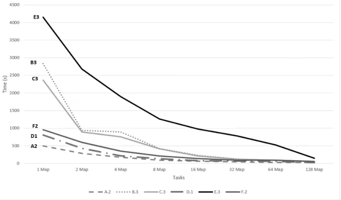
FIGURE 10: Scalability of BoaT programs. The trends show that BoaT program are able effectively leverage the underlying infrastructure.
To evaluate scalability we set up a Hadoop cluster with 23 nodes and with a capability of running 220 map tasks. We select one BoaT program from each category in Figure 5. Then we run the programs gradually increasing number of map tasks. The result of running the programs
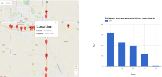
(a) Markers show the location of different speeding incidents. Once a marker is clicked the chart on the right side shows the number high-speed incidents categorized by speeds. This visualization is created from the result of the Task F.1
(b) Chart shows the counties with higher average speed on a day. This visualization is created from result of the Task D.2
FIGURE 11: Visualization of tasks F.1 and D.2
is shown in Figure 10. The vertical axis represents the time in seconds. We see as the number of maps increases the run time of the program decreases.
Example Dashboard Visualization
BoaT query results can be used to create interactive visualizations and dashboards. To support this claim we present few examples of simple visualizations.
We present the query result from Task F.1 in a simple dashboard created using JavaScript and Google Map in Figure 11(a). The markers show different speeding incident locations. Once a
FIGURE 12: This Tableau dashboard shows the road temperatures in degree Celsius at different times of the day at different locations. We can select the time from the time selector panel on the right. And once hovering the marker we’ll be able to see the road temperature at that location at that time.
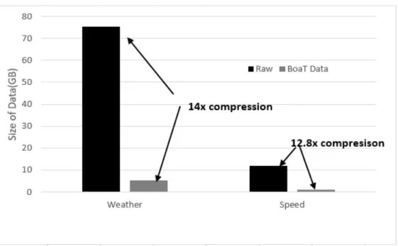
FIGURE 13: Reduction in data storage size in BoaT data infrastructure compared to the raw data
marker is clicked then the chart on the right side shows the number of vehicles recorded above 70 mph at that location. For example at location (41.97399057, -93.5702799) more than 150 vehicles were running at 71 mph on that day.
We provide another visualization of task D.2 in Figure 11(b). In this task, we find out the top ten counties where the average speed was higher than other counties on that day. BoaT result can be easily imported to Tableau or other visualization softwares to show the results. To show an example of this we visualize the result of task A.5 in the tableau in Figure 12. DOTs and researchers who use visualization tools like tableau can directly benefit from the BoaT results. Storage Efficiency
For evaluating the benefit we compare raw data along with the data storage in BoaT. If we compress the raw data to reduce the size we would lose the performance of query therefore a compressed format is not desirable. But in BoaT, we can achieve the desired performance even after a huge reduction in the data size. The language reads the objects according to the domain type and emits the result from the Hadoop nodes to produce the final result. For comparison, we used weather and speed data of one week for the state of Iowa. The weather data contains different weather information related grids at different locations at five minutes interval. The speed data contains the readings from Inrix sensors at 20 second intervals. The pre-processed raw weather data size 75.5 GB and the pre-processed raw speed data size is 12.07 GB. We took these datasets to generate an example BoaT dataset. On top of the raw weather and speed data, we add a lot more other data like county names of grids, county code, county names where the speed detector is located, road names of speed detectors. We collect some of this additional information from other metadata sources and some others using Google API. Even after adding a lot more additional data our generated BoaT dataset size is much smaller than the original raw data. The original 75.5 GB speed dataset is reduced to 5.38 GB in BoaT and the original 12.07 Gb speed dataset is reduced to 942 MB in BoaT as shown in Figure 13
CONCLUSION AND FUTURE WORK
Big Data-driven transportation engineering is ripe with potential to make a significant impact. However, it is hard to get started today. In this work, we have proposed BoaT, a transportation-specific Big Data programming language that is designed from the ground up to simplify express-ing data analysis task by abstractexpress-ing away the tricky details of data storage strategies, paralleliza-tion, data aggregaparalleliza-tion, etc. We showed the utility of our new approach, as well as its scalability advantages. Our future work will try out more application as well as create a web-based infras-tructure so that others can also take advantage of BoaT’s facilities.
ACKNOWLEDGEMENTS
This material is based upon work supported by the National Science Foundation under Grant CCF-15-18897 and CNS-15-13263. Any opinions, findings, and conclusions or recommendations ex-pressed in this material are those of the authors and do not necessarily reflect the views of the National Science Foundation.
REFERENCES
[1] Jagadish, H., J. Gehrke, A. Labrinidis, Y. Papakonstantinou, J. M. Patel, R. Ramakrishnan,
and C. Shahabi, Big data and its technical challenges.Communications of the ACM, Vol. 57,
No. 7, 2014, pp. 86–94.
[2] Lv, Y., Y. Duan, W. Kang, Z. Li, and F.-Y. Wang, Traffic flow prediction with big data: a deep
learning approach.IEEE Transactions on Intelligent Transportation Systems, Vol. 16, No. 2,
2015, pp. 865–873.
[3] Seedah, D. P., B. Sankaran, and W. J. O’Brien, Approach to Classifying Freight Data
Ele-ments Across Multiple Data Sources.Transportation Research Record: Journal of the
Trans-portation Research Board, , No. 2529, 2015, pp. 56–65.
[4] Zhang, J., F.-Y. Wang, K. Wang, W.-H. Lin, X. Xu, and C. Chen, Data-driven intelligent
transportation systems: A survey.IEEE Transactions on Intelligent Transportation Systems,
Vol. 12, No. 4, 2011, pp. 1624–1639.
[5] Barai, S. K., Data mining applications in transportation engineering. Transport, Vol. 18,
No. 5, 2003, pp. 216–223.
[6] Kitchin, R., The real-time city? Big data and smart urbanism. GeoJournal, Vol. 79, No. 1,
2014, pp. 1–14.
[7] Fan, J., F. Han, and H. Liu, Challenges of big data analysis.National science review, Vol. 1,
No. 2, 2014, pp. 293–314.
[8] Laney, D., 3D data management: Controlling data volume, velocity and variety.META Group
Research Note, Vol. 6, 2001, p. 70.
[9] Chen, C. P. and C.-Y. Zhang, Data-intensive applications, challenges, techniques and
tech-nologies: A survey on Big Data.Information Sciences, Vol. 275, 2014, pp. 314–347.
[10] Wang, S., S. Knickerbocker, and A. Sharma, Big-Data-Driven Traffic Surveillance System
for Work Zone Monitoring and Decision Supporting, 2017.
[11] Chakraborty, P., J. R. Hess, A. Sharma, and S. Knickerbocker,Outlier Mining Based Traffic
Incident Detection Using Big Data Analytics, 2017.
[12] Liu, C., B. Huang, M. Zhao, S. Sarkar, U. Vaidya, and A. Sharma, Data driven exploration of
traffic network system dynamics using high resolution probe data. InDecision and Control
(CDC), 2016 IEEE 55th Conference on, IEEE, 2016, pp. 7629–7634.
[13] Huang, T., S. Wang, and A. Sharma, Leveraging high-resolution traffic data to understand
the impacts of congestion on safety. In17th International Conference Road Safety On Five
Continents (RS5C 2016), Rio de Janeiro, Brazil, 17-19 May 2016, Statens väg-och transport-forskningsinstitut, 2016.
[14] Adu-Gyamfi, Y. O., A. Sharma, S. Knickerbocker, N. R. Hawkins, and M. Jackson,A
Frame-work for Evaluating the Reliability of Wide Area Probe Data, 2017.
[15] Dyer, R., H. A. Nguyen, H. Rajan, and T. N. Nguyen, Boa: Ultra-Large-Scale Software
Repository and Source-Code Mining. ACM Trans. Softw. Eng. Methodol., Vol. 25, No. 1,
2015, pp. 7:1–7:34.
[16] US Department of Transportation, Data Inventory, 2017, https://www.
transportation.gov/data.
[17] Biuk-Aghai, R. P., W. T. Kou, and S. Fong, Big data analytics for transportation: Problems
and prospects for its application in China. InRegion 10 Symposium (TENSYMP), 2016 IEEE,
[18] Kambatla, K., G. Kollias, V. Kumar, and A. Grama, Trends in big data analytics.Journal of Parallel and Distributed Computing, Vol. 74, No. 7, 2014, pp. 2561–2573.
[19] Dean, J. and S. Ghemawat, MapReduce: simplified data processing on large clusters.
Com-munications of the ACM, Vol. 51, No. 1, 2008, pp. 107–113.
[20] Pike, R., S. Dorward, R. Griesemer, and S. Quinlan, Interpreting the data: Parallel analysis
with Sawzall.Scientific Programming, Vol. 13, No. 4, 2005, pp. 277–298.
[21] Urso, A.,Sizzle: A compiler and runtime for Sawzall, optimized for Hadoop, 2012.
[22] El Faouzi, N.-E., H. Leung, and A. Kurian, Data fusion in intelligent transportation systems:
Progress and challenges–A survey.Information Fusion, Vol. 12, No. 1, 2011, pp. 4–10.
[23] Zheng, Y., Methodologies for cross-domain data fusion: An overview.IEEE transactions on
big data, Vol. 1, No. 1, 2015, pp. 16–34.
[24] Borning, A., H. Ševˇcíková, and P. Waddell, A domain-specific language for urban
simula-tion variables. InProceedings of the 2008 international conference on Digital government
research, Digital Government Society of North America, 2008, pp. 207–215.
[25] Borning, A., P. Waddell, and R. Förster, UrbanSim: Using simulation to inform public
delib-eration and decision-making.Digital government, 2008, pp. 439–464.
[26] Waddell, P., A. Borning, M. Noth, N. Freier, M. Becke, and G. Ulfarsson, Microsimulation of
urban development and location choices: Design and implementation of UrbanSim.Networks
and spatial economics, Vol. 3, No. 1, 2003, pp. 43–67.
[27] Simmhan, Y., S. Aman, A. Kumbhare, R. Liu, S. Stevens, Q. Zhou, and V. Prasanna,
Cloud-based software platform for big data analytics in smart grids.Computing in Science &
Engi-neering, Vol. 15, No. 4, 2013, pp. 38–47.
[28] Du, B., R. Huang, X. Chen, Z. Xie, Y. Liang, W. Lv, and J. Ma, Active CTDaaS: A Data
Ser-vice Framework Based on Transparent IoD in City Traffic.IEEE Transactions on Computers,
Vol. 65, No. 12, 2016, pp. 3524–3536.
[29] Yang, J. and J. Ma, A big-data processing framework for uncertainties in transportation data. InFuzzy Systems (FUZZ-IEEE), 2015 IEEE International Conference on, IEEE, 2015, pp. 1–6.
[30] Wang, X. and Z. Li, Traffic and Transportation Smart with Cloud Computing on Big Data. IJCSA, Vol. 13, No. 1, 2016, pp. 1–16.