Short-Term Price Forecasting For Agro-products Using Artificial Neural Networks

(1)

Agriculture and Agricultural Science Procedia 1 (2010) 278–287

International Conference on Agricultural Risk and Food Security 2010

Short-Term Price Forecasting For Agro-products Using

Artificial Neural Networks

Gan-qiong Li

a,b*

, Shi-wei Xu

a,b

, Zhe-min Li

a,b

a

Agricultural Information Institute ,the Chinese Academy of Agricultural Sciences, China

b

Making accurate predictions for short-term market prices of agro-products is not a trivial task as several influencing factors have to be considered, especially many sudden factors which are difficult to be known in advance have a decided influence on the fluctuation of short-term prices. The short term violent fluctuation of agro-products will have some negative impacts on production, consumption as well as social stability. In china the production of agriculture is not only scattered but also small in scale, making the farmers face great market risk. In most cases the farmers are price takers not price makers, therefore the conditions of market may be opposite to the initial when agro-products had been produced. A well known fact is that short-term market price forecasting has been a challenge for many decades. Nikolay Arcak and Panagiotis G.

Key Lab of Digital Agricultural Early Warning Technology, Ministry of Agriculture, China

Abstract

It is well known that short-term market price forecasting has been a difficult problem for a long time because of too many factors which can not be accurately predicted. Conventionally, time series analysis has been often employed in modeling short-term price forecasts. In recent years a new technique of artificial neural networks˄ANN˅has been proposed as an efficient tool for modeling and forecasting. A feed-forward ANN model has been developed for short-term price forecasting of tomato and in comparison with time series model ARIMA in this study. The data used include daily wholesale price, weekly wholesale price and monthly wholesale price collected between 1996 and 2010. The results showed that ANN model evidently outperformed the time series model in forecasting the price before one day or one week. A good correlation between the modeled and the real prices was observed from the feed-forward ANN model, with a relative error less than 5.0%.

Key words: short-term forecasting, neural networks, regression analysis, time series analysis, model;

1. Introduction

[1]

attempted to model volatility in prediction markets. Generally most researchers prefer to use leaner techniques such as regression models and time series models since its easy using. Nowadays short term forecasting is used popularly in many fields such as electric load, traffic flow, stock exchange, water demand, disaster and whether [2-11]

*

Corresponding author, Tel.: 010-82109761; fax: 010-82106285

. The short-term forecasting model has always

E-mail address: lgqxjf@caas.net.cn

Open access under CC BY-NC-ND license.

(2)

been applied to agro-product price forecasting before one month or one quarter, but rarely applied to that before several days or one week.

Short term price forecasting for agro-products is a subject that has been studied extensively since 21 century, and several different methods have been developed. Conventional statistical forecasting methods can be divided into linear regression method and time series method. In the simple or multiple regression model, the relationships between the dependent variables and independent variables are modelled. The parameters are estimated according to the past values of these variables, and the relationships are used to forecast the dependent variable by using the future evaluations of the independent ones. In fact, linear regression models have a significant drawback. The market price of agro-products has multiple influencing factors which have complex inter-relations. In regression models it was assumed that the explanatory variables and dependent variable are linear relationships. However, they are more or less nonlinear. In the time series methods such as persistence method, trends method, the prediction is based on the past values. Taking persistence method for example, the main idea is today equals tomorrow, i.e. if the wholesale price of tomato is 2.50 Yuan/kg today, the persistence method predicts that it will be 2.50 Yuan/kg tomorrow. This method works well when factors of market change very little. However, if market conditions change significantly from day to day, this method usually breaks down. Trends method also has some drawback because the conditions did not continue to move in the same direction simultaneously. If they slow down, speed up, change intensity, or change direction, the trends forecasting probably will not work as well. Paulo cortez [12]employed

evolving time series forecasting ARMA models to overcome some shortage mentioned above. Qun zhou et al[13]

proposed a two-stage approach for generating simulated price scenarios based on the available price date, and their results indicated that the proposed approach was able to generate price scenarios for distinct seasons with

empirically realistic characteristics.

Real-world price data of agro-products and its underlying market changes are often nonlinear in nature. As a result, linear models may not be suitable when market changes frequently. The rapid development of computing power has allowed nonlinear method to become applicable to modelling and forecasting. The artificial neural network (ANN) with a nonlinear dynamics system is based on the distributive storage and parallel co-processing of messages. Recently, numerous artificial neural networks in modelling the complex nonlinear relationships between the market price and its determining factors such as meteorological and seasonal variables, holidays, food safety cases and other emergencies have been reported[14-25]

%

100 u

obs obs f error

X

P

.

The main objective of this study is to examine whether ANN model is suitable for short-term forecasting and how its accuracy is compared with time series model. Historical forecasting and future forecasting were used here. The historical forecasting is mainly to evaluate the fitness of the two methods based on historical data, and the future forecasting is to examine the accuracy of forecasting results based on the two models.

2. Date Processing and Evaluation Methods of Model

Tomato was used as a target throghout this study because it is one of the most popular and familiar agro-products in China. Historical data employed in the study were available on the websit of Ministry of Agriculture (MOA) of China, where the database included tomatoes’ daily price of 511 wholesale markets of agro-products in China since 1996. Because there were short of daily volumes of tomatoes’ trade for some wholesale market, the whole country daily wholesale price of tomatoes was an arithmetical average of 511 wholesale markets. The weekly wholesale price and monthly wholesale price of the whole country were also calculated by the same method.

To evaluate the fitness of different models, we used relative error as an important index to compare them. The relative error is calculated as follows:

error

P

means relative error.

X

f is the fit of model simulation.

X

obs is the real observation.

3. Time Series Model 3.1 Simple Description

The time series analysis ARIMA model is popularly applied in short term forecasting since it doesn’t need too much economics knowledge for the users. In the following paragraph we used the method to establish daily price forecasting model, weekly price forecasting model and monthly price forecasting model by PASW Statistic 18.0.

(3)

3.2 Historical forecasting and Evaluation A. Daily Price Forecasting Model

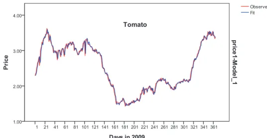
According to the data of 365 daily price in 2009, a suitable model of ARIMA˄0,1,7˅can be established by

PASW Statistic 18.0. Figure 1 shows the results of simulation on daily price. The accuracy distribution of historical prediction is listed below:

1) The relative error between 10% and 15% was 5, indicating that the proportion of prediction accuracy between 85% and 90% was 1.4 percent of the total historical forecasting for daily price.

2) The relative error between 5% and 10% was 22, indicating that the proportion of prediction accuracy between 90% and 95% was 6.0 percent of the total historical forecasting for daily price.

3) The relative error less than 5% was 337, indicating that the proportion of prediction accuracy more than 95% was 92.6 percent of the total historical forecasting for daily price.

Figure 1: historical forecasting for daily wholesale price using ARIMA model B. Weekly Price forecasting Model

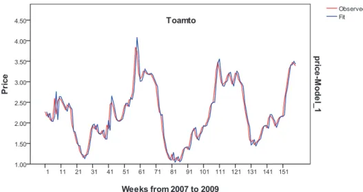
According to the data of weekly price from 2007 to 2009, a suitable model of ARIMA˄1,1,0˅can be

established by PASW Statistic 18.0. Figure 2 shows the results of simulation on weekly price. The accuracy distribution of historical prediction is listed below:

1) The relative error between 20% and 25% was 5, indicating that the proportion of prediction accuracy between 75% and 80% was 3.2 percent of the total historical forecasting for weekly price.

4) The relative error less than 5% was 91, indicating that the proportion of prediction accuracy more than 95% was 57.5 percent of the total historical forecasting for weekly price.

(4)

Figure 2: historical forecasting for weekly wholesale price using ARIMA model C. Monthly Price Forecasting Model

According to the data of monthly price from 1996 to 2009, a suitable model of ARIMA˄0,1,2˅˄1,1,1˅s

can be established by PASW Statistic 18.0. Figure 3 shows the results of simulation on monthly price. The accuracy distribution of current prediction is listed below:

1) The relative error more than 30% was only 1, indicating that the proportion of prediction accuracy less than 70% was 0.7 percent of the total historical forecasting for monthly price.

2) The relative error between 20% and 30% was 14, indicating that the proportion of prediction accuracy between 70% and 80% was 9.0 percent of the total historical forecasting for monthly price.

5) The relative error less than 5% was 53, indicating that the proportion of prediction accuracy more than 95% was 34.2 percent of the total historical forecasting for monthly price.

(5)

4. ANN model

The ANN usually called “neural network” (NN), is a mathematical model or computational model that tries to simulate the structure and/or functional aspects of biological neural networks. It consists of an interconnected group of artificial neurons and processes information using a connectionist approach to computation. In most cases an ANN is an adaptive system that changes its structure based on external or internal information that flows through the network during the learning phase. Modern neural networks are non-linear statistical data modelling tools. They are usually used to model complex relationships between inputs and outputs or to find patterns in data.

A feed-forward neural network is one of ANN where connections between the units do not form a directed cycle. In this network, the information moves in only one direction, forward, from the input nodes, through the hidden nodes (if any) and to the output nodes. There are no cycles or loops in the network. Now feed-forward neural network is the most popular and most widely used model in many practical applications. In this study, feed-forward neural network is used as the forecasting network.

4.1 Algorithm Steps

The basic flow chart of ANN is shown as below:

Network Training Initial Network Trained Network Evaluation Data Network Forecasting Data Pre-process Initial Data Sample Data Input Data Forecasting Result Evaluation Result

The steps of price forecasting are listed as follows:

1) Data Pre-processing: Since poor or insufficient data were not suitable to develop good models, the initial data should be pre-processed before applying neural network algorithm. Here we only carry on data normalization in the pre-processing step (

V

mean

x

y

,

V

is the standard deviation, and x is the input data). Usually we

can divide the initial data into two parts: sample data (used in network training) and validation data (used in network evaluation).

2) Neural Network Creation: In this study a three-layer feed-forward neural network including input layer, hidden layer and output layer was used. The number of neurons in input and output layer depends on practical application. In our study, the neuron number of input layer and output layer should be set as nand mif we want to

forecast the price of next mdays based on the price of past ndays. And according to that, the neuron number of

hidden layer should be set as (2hn+ 1) based on Kolmogorov Theorem.

3) Neural Network Training: During the neural network training step, firstly we should determine the value of two important parameters. One is the Mean Squared Error (MSE), which represents the average squared error between the network's output and the target value. The other is the maximum number of learning epochs, up to which the training will be stopped no matter whether the mean-squared error target has been achieved. Now we can train the neural network with the sample data generated in Step 1. The training phase will stop when the mean-squared error is achieved or the maximum number of learning epochs is reached.

(6)

agricultural commodity price.

4.2 Historical Forecasting and Evaluation A. Daily Price Forecasting

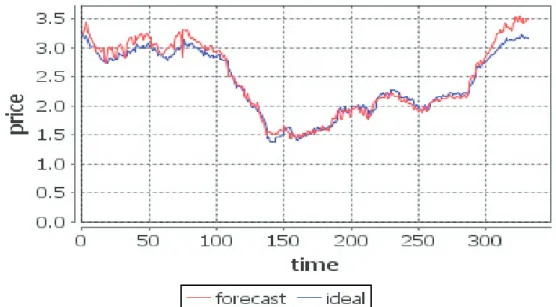
The data of daily price from 1996 to 2008 were used as sample date (network training) and the data of 2009 were used as historical prediction model evaluation (network evaluation). Figure 4 shows the results of simulation on daily price. The accuracy distribution of historical prediction is listed below:

1) The proportion of prediction accuracy between 85% and 90% was 2.1 percent of the total historical forecasting for daily price.

2) The proportion of prediction accuracy between 90% and 95% was 29.9 percent of the total historical forecasting for daily price.

3) The proportion of prediction accuracy more than 95% was 68.0 percent of the total historical forecasting for daily price.

Figure 4: Forecasting for daily wholesale price of tomatoes using ANN B. Weekly Price Forecasting

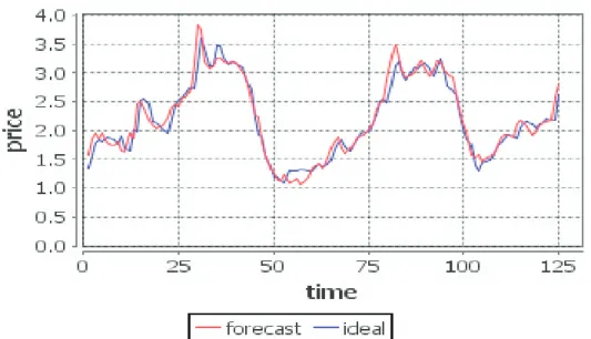
Tthe data of weekly price from 1996 to 2006 were used as sample data (network training) and the weekly data between 2007 and 2009 were used as historical prediction model evaluation (network evaluation). Figure 5 shows the results of simulation on weekly price. The accuracy distribution of historical prediction is listed below:

1) The proportion of prediction accuracy between 75% and 80% was 2.4 percent of the total historical forecasting for weekly price.

4) The proportion of prediction accuracy more than 95% was 61.6 percent of the total historical forecasting data of weekly price.

(7)

Figure 5: Forecasting for weekly wholesale price of tomatoes using ANN C. Monthly Price Forecasting

The data of monthly price from 1996 to 2009 were used as sample data (network training) and historical prediction evaluation (network evaluation). Figure 6 shows the results of simulation on monthly price. The accuracy distribution of historical prediction is listed below:

1) The proportion of prediction accuracy less than 70% was 8.1 percent of the total historical forecasting for monthly price.

2) The proportion of prediction accuracy between 70% and 80% was 14.3 percent of the total historical forecasting for monthly price.

5) The proportion of prediction accuracy above 95% was 31.7 percent of the total historical forecasting for monthly price.

(8)

5. Future Forecasting and Conclusions 5.1 Future Forecasting Results

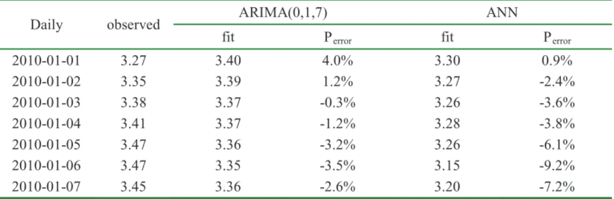
Applying the above models of ARIMA and ANN, the forecasting results ahead of seven days for 2010 are listed in table 1. Table 2 is the results ahead of four weeks and table 3 is the results ahead of three months.

As we can seen from table 1, ARIMA model and ANN model are both effective for forecasting daily price and the accuracy is more than 90%. The accuracy of ANN model declines with the longer forecasting cycles.

Table 1: Comparison of Future Forecasting Results of Tomatoes’ Daily Wholesale Price between ARIMA and ANN

Daily observed ARIMA(0,1,7) ANN

fit Perror fit Perror

2010-01-01 3.27 3.40 4.0% 3.30 0.9% 2010-01-02 3.35 3.39 1.2% 3.27 -2.4% 2010-01-03 3.38 3.37 -0.3% 3.26 -3.6% 2010-01-04 3.41 3.37 -1.2% 3.28 -3.8% 2010-01-05 3.47 3.36 -3.2% 3.26 -6.1% 2010-01-06 3.47 3.35 -3.5% 3.15 -9.2% 2010-01-07 3.45 3.36 -2.6% 3.20 -7.2%

As we can seen from table 2, the accuracy of ANN model in forecasting weekly price is lower than that of ARIMA model. The accuracy of ANN model declines rapidly with the longer forecasting cycles.

Table 2: Comparison of Future Forecasting Results of Tomatoes’ Weekly Wholesale Price between ARIMA and ANN

Weekly observed ARIMA(1,1,0) ANN

2010-1 3.40 3.37 -0.9% 3.35 -1.5%

2010-2 3.39 3.37 -0.6% 3.25 -4.1%

2010-3 3.51 3.36 -4.3% 3.24 -7.7%

2010-4 3.55 3.36 -5.4% 3.07 -13.5%

As we can seen from table 3, ARIMA model and ANN model are both not very ideal comparing with daily price forecasting and weekly price forecasting.

Table 3: Comparison of Future Forecasting Results of Tomatoes’ Monthly Wholesale Price between ARIMA and ANN

Monthly observed ARIMA(0,1,2)(1,1,1) ANN

s

2010-01 3.46 3.70 6.9% 3.55 2.6%

2010-02 3.47 3.87 11.5% 3.74 7.8%

2010-03 3.26 3.86 18.4% 3.79 16.3%

5.2 Conclusions

y The time interval of data is shorter, the accuracy is higher. Results showed the accuracy of daily price

forecasting is the best. Next is weekly price forecasting.

y The ANN model is more suitable for forecasting ahead of one cycle. Time series model and ANN model

are equally effective in accuracy for forecasting ahead of one day, one week and one month, but ANN model is better than time series model.

y The accuracy of ANN model for three types of forecasting is more than 80%, and daily price forecasting is

(9)

6. Discussions

Although ANN is an effective tool for short term forecast and widely used in many fields nowadays, there are still some problems to be further solved.

y Disadvantages

ANN is in a sense the ultimate ‘black boxes’. Apart from defining the general architecture of a network and perhaps initially seeding it with a random numbers, the user has no other role than to feed it input and watch it train and await the output. In fact, it has been said that with ANN, “you almost don't know what you're doing”. The final product of this activity is a trained network that provides no equations or coefficients defining a relationship (as in regression) beyond it's own internal mathematics. The network 'IS' the final equation of the relationship.

y Potential Improvements

Firstly, we only carried out normalization on the initial data in Step 1. Considering the difficulty of obtaining the price data of each day, we can carry out data smoothing on the price-time curve to gain the missing day’s data.

Secondly, feed-forward neural network is the most widely used models, but it has the simplest network architecture. So if the price-time curve presents a more

1. Nikolay Archak and Panagiotis G.. lpeirotis. Modeling Volatility in Prediction Markets. Ec’09, July 6-10, 2009,

Stanford, California, U.S.A.

sophisticated shape, we can attempt to apply more complicated types of network on this problem.

Finally, now we only train the network once before using it to forecast price. In order to minimize the instability of neural network, we can carry on a few times of training and forecasting, and use the average value of each time as the final predicted output.

Acknowledgement

This work is supported by Key Project of National Key Technology R&D Program--“Support System and Demonstration of Key Technologies of Intelligent-Analysis and Early-Warning for Security of Agro- Products” of China with Project 2009BADA9B01.

Referances

2. S.Kuusisto, M.Lehtokangas, J. Saarinen and K. Kashi. Short Term Electric Load Forecasting Using a Neural

Network with Fuzzy Hidden Neurons. Neural Comput & Applic, 6: 42-56, 1997.

3. Shiliang Sun. Traffic Flow Forecasting Based on Multitask Ensemble Learning. GEC’09, June 12-14, 2009,

Shanghai, China.

4. George S. Atsalakis and Kimon P. Valavanis. Forecasting Stock Market Short-term Trends Using a

Neuro-fuzzy Based Methodology. Expert Systems with Applications, Volume 36, Issue 7, September 2009, pp. 10696-10707.

5. Ignacio J. Ramirez-Rosado, L. Alfredo Fernandez-Jimenez, Cláudio Monteiro, João Sousa, and Ricardo Bessa.

Comparison of Two New Short-term Wind-power Forecasting Systems. Renewable Energy, Volume 34, Issue 7, July 2009, pp.1848-1854.

6. Ahmed Eman. Optimal Artificial Neural Network Topology for Foreign Exchange Forcasting. ACM-SE’08,

March 28-29, 2008, Auburn, AL, U.S.A.

7. Ashu Jain, Ashish Kumar Varshney and Umesh Chandra Joshi. Short-Term Water Demand Forecast Modeling

at IIT Kanpur Using Artificial Neural Networks. Water Resources Management, 15: 299-321, 2001.

8. Ivan Simeonov, Hristo Kilifarev and Rajcho llarionov. Algorithmic Realization of System for Short-term

weather forecasting. CompSysTech’07. June 14-15, 2007. University of Rousse, Bulgaria.

9. Chiristopher Kiekintveld, Jason Miller, Patrick R. Jordan and Michael P. Wellman. Forecasting Market Price in

a Supply Chain Game. AAMAS’07 May14-18 2007, Honolulu, Hawai’i, U.S.A.

10. Trino-ManuelϿoguez. Volatility and VaR forecasting in the Madrid Stock Exchange. Span Econ Rev,

10:169-296, 2008.

11. Tezuka Massaru and Munakata Satoshi. Daily Demand Forecasting of New Products Utilizing Diffusion Models and Genetic Algorithms. SAC’09 March 8-12, 2009, Honolulu, Hawai’i, U.S.A.

12. Paulo Cortez. Evolving Time Series Forecasting ARMA Models. Journal of Heuristics, 10: 415-429, 2004. 13. Qun Zhou, Leigh Tesfatsion and Chen-Ching Liu. Scenario Generation for Price Forecasting in Restructured

wholesale power markets. 2009 Power systems Conference & Exposition, March 15-18, 2009, Seattle, Washington, U.S.A.

14. Farzan Aminian, E.Dante Suarez, Mehran Aminian and Daniel T. Walz. Forecasting Economic Data with Neural Networks. Computational Economics, 28: 71-88, 2006.

(10)

15. Matthew Butler and Ali Daniyal. Multi-objective Optimization with an Evolutionary Artificial Neural Network for Financial Forecasting. GECCO’09, July 8-12, 2009, Montreal Quebec, Canada.

16. Zhou Zhina, Shi Zhongke and Li Yingfeng. Study to Short-term Flow Estimation at Intersection Base on Genetic Neural Networks. GEC’09, June 12-14, 2009, Shanghai, China.

17. Philippe Lauret, Eric Fock, Rija N. Randrianarivony, and Jean-François Manicom-Ramsamy. Bayesian Neural Network Approach to Short Time Load Forecasting. Energy Conversion and Management, Volume 49, Issue 5, May 2008, pp. 1156-1166.

18. Raúl Pino, José Parreno, Alberto Gomez and Paolo Priore. Forecasting Next-day Price of Electricity in the Spanish Energy Market Using Artificial Neural Networks. Engineering Applications of Artificial Intelligence, Volume 21, Issue 1, February 2008, pp. 53-62.

19. Coúkun Hamzaçebi. Improving Artificial Neural Networks’ Performance in Seasonal Time Series Forecasting.

Information Sciences, Volume 178, Issue 23, December1, 2008, pp. 4550-4559.

20. R.E. Abdel-Aal. Univariate Modeling and Forecasting of Monthly Energy Demand Time Series Using Abductive and Neural Networks. Computers & Industrial Engineering, Volume 54, Issue 4, May 2008, pp. 903-917.

21. J.P.S. Catalão, S.J.P.S. Mariano, V.M.F. Mendes, and L.A.F.M. Ferreira. Short-term Electricity Prices Forecasting in a Competitive Market: A Neural Network Approach. Electric Power Systems Research, Volume 77, Issue 10, August 2007, pp. 1297-1304.

22. Paras Mandal, Tomonobu Senjyu, and Toshihisa Funabashi. Neural Networks Approach to Forecast Several Hour Ahead Electricity Prices and Loads in Deregulated Market. Energy Conversion and Management, Volume 47, Issues 15-16, September 2006, pp. 2128-2142.

23. Yevgeniy Bodyanskiy and Sergiy Popov. Neural Network Approach to Forecasting of Quasiperiodic Financial Time Series. European Journal of Operational Research, Volume 175, Issue 3, December 16, 2006, pp. 1357-1366.

24. David Enke and Suraphan Thawornwong. The Use of Data Mining and Neural Networks For Forecasting Stock Market Returns. Expert Systems with Applications, Volume 29, Issue 4, November 2005, pp.927-940.

25. T. Yalcinoz and U. Eminoglu. Short Term and Medium Term Power Distribution Load Forecasting By Neural Networks. Energy Conversion and Management, Volume 46, Issues 9-10, June 2005, pp. 1393-1405.