M
IMICKING
C
REDIT
R
ATINGS
BY A
P
ERPETUAL
-D
EBT
S
TRUCTURAL
M
ODEL
G
AIA
B
ARONE
August 8, 2017 LUISS Guido Carli: Research project
Field:Credit, banking, risk management
1. RATINGS AND DEFAULT FREQUENCIES... 3
2. PERPETUAL-DEBT MODEL ... 6
3. MODEL’S ESTIMATES ... 8
4. SOME STYLIZED FACTS ... 10
5. AFIRM-LEVEL APPLICATION: THE DEUTSCHE BANK CASE. ... 11
6. CONCLUSIONS ... 15
REFERENCES ... 17
Gaia Barone
Mimicking Credit Ratings
by a Perpetual-Debt Structural Model
Gaia Barone
GAIA BARONE
ADVANCED FINANCIAL MATHEMATICS
LUISS - Guido Carli University of Rome
gbarone@luiss.it
In this paper, we outline the general lines of a structural model that is based on the Leland model (1994), but differs from its assumptions about the tax regime. In the revised model, which we call the Perpetual-Debt Structural Model (PDSM), stocks are equivalent to a portfolio that contains a perpetual American option to default.
This paper offers a first empirical test of the model. Es-sentially, the question is: “Is the PDSM sufficiently flexible to give default probabilities consistent with those historically estimated by Moody’s?”. As we will see, the answer is posi-tive.
The paper contains a simple firm-level application. The PDSM risk indicators have been used to define the “market rating” of Deutsche Bank.
n 1979, Modigliani and Cohn ([15], p. 24) argued that stock prices were undervalued by 50%: the S&P 500 index, which was equal to about 100 at the end of 1977, should have been equal to 200, a level that was actually reached in November 1985, about 8 years later. Their analysis was based on a simple model of capitalizing current earnings: “... one possible way to value the firm’s equity under inflation is to capitalize ‘true’ profits at the capitalization rate that applies in the absence of inflation” ([15], p. 31).
A few years before 1979, Black and Scholes ([6]) and Merton ([13]) had proposed a more complex valuation model that took into account the optionality of stock investments. Common stocks were viewed as call options on a firm’s assets. As an alternative, by the put-call parity, stocks can be viewed as a portfolio made up of a “long” forward, by means of which stock-holders commit themselves to buy back the firm’s assets from the bondstock-holders, and a “long” put, i.e. an option to default that allows shareholders to declare bankruptcy to avoid having to buy back the firm’s assets at a price higher than their market value.1
1 See Black and Scholes ([6], p. 649): «It is not generally realized that corporate liabilities other than
warrants may be viewed as options. Consider, for example, a company that has common stock and bonds outstanding ... it is clear that the stockholders have the equivalent of an option on their com-pany’s assets. In effect, the bond holders own the company's assets, but they have given options to the stockholders to buy the assets back.». See also Merton ([13], p. 178): « ... we can use the total value of the firm as a “basic” security ... and the individual securities within the capital structure (e.g., debt, convertible bonds, common stock, etc.) can be viewed as “options” or “contingent claims” on the firm and priced accordingly.».
The first to successfully implement the Black-Scholes-Merton intuition were Kealhofer-McQuown-Vašíček, known by the acronym KMV, the name of the firm sold to Moody’s in 2002 for $210 million.
In order to implement the KMV model, the face value and the maturity of the firm’s debt must be defined. In addition, the stock’s volatility has to be estimated. In this model, both the default point and the possible default time are exogenously given. Insolvency occurs if, at the debt’s maturity (1 year, by hypothesis), the value of the assets is lower than the face value of the debt, which is assumed to be equal to the book value of the short-term debt (up to 1 year) plus a certain share of the long-term debt.2
In 1994, Leland ([12]) proposed a model that, in the writer’s opinion, is theoretically more appealing than the KMV model. In the Leland model, differently from the KMV model, it is assumed that bonds, like stocks, are perpetual securities.3
Therefore, it is assumed that the complex debt structure of a firm can be approximated by a fixed-rate perpetual bond, with a certain nominal value. The assumption of a perpetual debt is justified not only for the sake of simplicity, but also because firms are normally able to roll over their debts.
The main advantages of the Leland model, compared with the KMV model, are two fold: 1) insolvency can occur at any instant of time; 2) the default point and the recovery rate are endogenous. In substance, compared with the KMV model, the Leland model greatly reduces the use of ad hoc assumptions (the maturity of the debt, the default point, the recovery rate).
While there have been several empirical tests of the archetype of the KMV model, i.e. the Merton model ([14]), one cannot say the same for Leland’s model. To the best of our knowledge, the only contribution is that of Forssbæck and Vilhelmsson ([8]), who compare the Leland and the Merton models, with results favorable to the latter.
The bad performance of the Leland model highlighted by the above paper can be at-tributed to its hypotheses about the fiscal setting, which entail an obvious drawback: the stock’s value rises if the tax rate rises.
Adopting a different tax-regime approach makes it possible to avoid this drawback, while maintaining the merits of the original model referred to above.
In the revised model, which has been fully described in other articles (Barone [2], [3], [4], [5]) and which we call Perpetual-Debt Structural Model (PDSM), stocks are equivalent to a portfolio that contains a perpetual American option to default.
In the Merton-KMV model, the option to default is European and has a finite-length ma-turity, equal to the maturity of the debt. This assumption makes it difficult to price contracts where stocks are the underlying asset.
2 See Moody’s ([18], p. 9): “The long-standing practice of defining the default point has been ‘current
liability + ½ long term liability.’ As part of the EDF9 research, we reevaluated the formula against many alternative possibilities. We found that the other approaches were not consistently better than the long-standing practice for non-financial firms. For financial-firms, however, ... we set the default point as a percentage of total adjusted liabilities. We calibrate that percentage as 75%.”.
3 On the convenience of an infinite time horizon, from the modeling’s standpoint, we can cite Kassouf
([11], p. 276): “Paradoxically, the case of finite-length options is much more difficult [Ed.: than the case of perpetual options], indicating once again that easy answers can sometimes be arrived at by ‘passing’ to infinity.”
§1 Ratings and Default Frequencies 3
Another merit of the PDSM, already embedded in the Merton-KMV model, is the fact that the distribution of stock returns changes over time, as a function of leverage: the greater the leverage, the greater the stock’s volatility. As a consequence, the theoretical prices of stock options can be consistent with the volatility smiles observed in the market.
Therefore, a single model makes it possible to consistently price both stocks and stock options. Besides, since the PDSM gives a closed-form formula for the default probabilities of any maturity, CDSs can also be consistently priced, without making any ad hoc assumption about the recovery rate, which is endogenously given by the model.
This paper offers a first empirical test of the model. Essentially, the question is: “Is the PDSM sufficiently flexible to give default probabilities consistent with those historically esti-mated by Moody’s?”. As we will see, the answer is positive.
Then we will look at a simple application where the PDSM is estimated at the level of a single listed firm, Deutsche Bank in our case. The model’s estimates, made in such a way as to obtain theoretical values in line with the market quotes and the balance-sheet data, make it possible to assign a “market-based” rating. As we will see, the rating of Deutsche Bank based on the PDSM is consistent with Moody’s rating.
The rest of this paper is organized as follows: after a section in which we examine the default frequencies for the rating classes defined by Moody’s (§1), the paper describes the Perpetual-Debt Structural Model (§2). The model’s estimates based on Moody’s default fquencies are then presented (§3). After describing some stylized facts that synthetize the re-sults obtained (§4) and illustrating the application of the PDSM to the case of Deutsche Bank (§5), the paper closes with some short final considerations (§6).
1. Ratings and Default Frequencies
The rating agencies bracket firms in a finite number of rating classes and annually compute, for each class, the default rate, i.e. the ratio between the number of historically observed defaults and the number of companies in the cohort formed at the beginning of the observation period. The rating is a discrete “qualitative” variable (i.e. a “categorical” statistic). If we wish to synthesize the financial health of a firm in a unique statistic, it might be better to define a con-tinuous “quantitative” variable rather than a discrete one. For example, the x-year probability of default, continuously defined between 0 and 1, could be a valid alternative to the rating, even if it measures only one aspect of the firm’s risk.
Actually, risk is a multi-dimensional concept (Barone [1]), and there are many other key variables that are useful in measuring it, such as asset volatility (or business risk), leverage (the ratio between after-tax assets and equity), equity volatility (the standard deviation of annual-ized equity returns), recovery rate (the complement to 1 of the loss given default), distance to default (the log distance from the default point), time to default (or distance from default).
It goes without saying that Moody’s rating classes (Aaa, Aa, A, Baa, Ba, B, Caa-C) repre-sent, so to speak, just as many “still-images” of a movie where the worsening of the rating and the correspondent increase of the default probability “go hand in hand” with the increase of business risk, leverage, equity volatility, and with the decrease of recovery rate, distance to de-fault, time to default.
Like human beings, firms are born, grow up, age, and then die. At the time of John Graunt (1620-1674), the 10-year death probability of an individual aged 46, defined as the probability of a person from a specific generation, exactly 46 years old, dying before reaching age 56, was equal to 40% [Rubinstein [20], pp. 30-33)]. In the period 1920 - 2010, Moody’s 10-year average default rate for all rated companies, defined as the probability of default from the time the pool of issuers is formed up to a 10-year time horizon, was equal to 11.811%. Death probabilities and default rates change over time as a function of welfare and the state of the economy, respectively. Now, as shown by the mortality tables ([21]), the death probabilities are much lower than they were at the time of John Graunt. Instead, life conditions for firms did not improve with the passage of time. On the contrary, in recent years, the average default rate for all rated companies increased slightly.
Mortality tables report the 1-year death probabilities by age of individuals. Instead, Moody’s matrices report the n-year (1 ≤n≤ 20) average cumulative (issuer-weighted) default rates by rating class.4 The default rates calculated ex post by Moody’s, on the basis of historical observations, can be interpreted as default probabilities, from an ex ante standpoint. More precisely, Moody’s matrices report the cumulative probabilities, Q(T), i.e. the probabilities that the firms with a certain rating at time 0 will default by a certain maturity T. Decumulating these probabilities, we can obtain the estimates of the annualunconditional default probabili-ties, qi [= Q(ti+1) −Q(ti)], i.e. the estimates of the probabilities that the firms with a certain
rat-ing at time 0 will default in the ithyear (i = 1, 2, ..., n). Finally, the conditional default
probabili-ties, λi {=qi / [1 −Q(ti−1)]}, measure the probability that the firms with a certain rating at time 0
will default in the ithyear, provided that they are still alive at the end of the previous year.
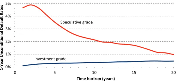
A striking fact inferred from the default rates reported by Moody’s is that – for invest-ment-grade firms – the 1-year unconditional default rate tends to be an increasing function of time, while the opposite is true for speculative-grade firms (Figure 1). Why? If a firm is consid-ered to be creditworthy, the more time elapses, the greater the possibility that its financial health will decline. Instead, for a firm with a poor credit rating, the next year or two may be criti-cal: the longer the firm survives, the greater the chance that its financial health will improve.
Moody’s analysis of default rates is further refined by distinguishing investment-grade and speculative firms by letter rating classes (Aaa, Aa, A, ...) and alphanumeric rating classes (Aa1, Aa2, Aa3, A1, A2, A3, ...). Moreover, default rates provided by Moody’s are adjusted to take account of rating withdrawals, “which occur when borrowers shift from rated public to unrated private debt finance or when all their debts are extinguished outright” (Hamilton and Cantor [9]), and are calculated by giving all issuers the same weight (“issuer-weighted” default rates) or by giving each exposure a weight proportional to the total value of its outstanding bonds (“volume-weighted” default rates). We will use the “issuer-weighted” default rates ([17], Exhibit 34, pp. 32-3)
4 Mortality tables also show life expectancies for individuals of any age. Similar calculations, as the
cal-culation of the expected time to default, are not possible for the firms considered by Moody’s. In Moody’s matrices, the maximum time horizon is 20 years, against 120 years in mortality tables. The maximum life of a firm can be measured in centuries (the oldest bank in continuous operation since its establishment is Monte dei Paschi di Siena, founded in 1472), while the oldest verified person ev-er didn’t reach the 120 years (in the U.S., Sarah Knauss lived 119 years and 97 days).
§1 Ratings and Default Frequencies 5
As mentioned in the introduction, we use Moody’s data to check whether the Perpetual-Debt Structural Model (PDSM) is sufficiently flexible to give default probabilities consistent with those historically estimated by Moody’s.
As will be seen, the model produces internally consistent values that smooth the “asper-ities” of Moody’s data, which are particularly “severe” in the case of conditional default rates (Figure 2).5
Moreover, the PDSM offers a closed-form formula to calculate the probability of default,
Q(T), for any time horizon T, with 0 < T < +∞ [Equation (4)]
5 The conditional default rates, λ, of Figure 2 have been calculated by applying the Equation (9) to the
data of Exhibit 34 in Moody’s ([17], pp. 32-33).
Figure 1 Moody’s 1-year average unconditional default rates (1970 - 2010).
Figure 2 Moody’s 1-year average conditional default rates. 0% 1% 2% 3% 4% 5% 0 5 10 15 20 1-Yea r U nc on di tio na l D ef au lt Ra tes
Time horizon (years)
Source: Moody's, Average Cumulative Issuer-Weighted Global Default Rates, 1970-2010. Speculative grade Investment grade 0% 5% 10% 15% 20% 0 5 10 15 20 1-Yea r C on di tio na l D ef au lt Ra tes
Time horizon (years)
Caa-C B Ba Baa A Aa Aaa
2. Model
The perpetual-debt model is a simple model where – unlike in other structural models – debt is modeled as a perpetual fixed-rate bond, instead of a zero-coupon bond with finite maturity (Barone ([3], [4]). Therefore, default can happen at any time, and not only at the bond’s ma-turity.
The state variable is represented by the value of the assets, V, which is assumed to fol-low a geometric Brownian motion with drift rate r – qV and variance rate σV2, where r is the
risk-free rate, qV is the payout rate and σV is the volatility of V.
The model (which belongs to the class of first-passage models) specifies default as the first time V hits a lower barrier, Vb, that is endogenously determined as a solution of an
opti-mal stopping problem (stockholders’ equity maximization). See Barone [5], pp. 65-66. Stockholders do have a perpetual American option to default.6
The assumption of an infinitely-lived security is not only convenient from a mathemati-cal and practimathemati-cal standpoint (there is no need to estimate the debt’s maturity parameter), but is also a good proxy for a short-term debt rolled over again and again, as with perpetual float-ers.
In the PDSM there are four stakeholders:
1. stockholders hold the residual claim on the firm’s assets, i.e. equity, whose current value is S0. They issue a perpetual bond with nominal value Z, coupon C = r Z, and market val-ue B0. Because of the firm’s limited liability, they have an option to default, that is the (perpetual) right to sell the assets at price Z to the bondholders. In other words, they have a perpetual American put option, with strike Z and market value P, written on V. When V = Vb, stockholders exercise their option to default. This prevents equity’s value
from becoming negative. When the (put) option is exercised, stockholders sell the firm’s assets, whose value is Vb, and receive Z from the bondholders;
2. bondholders hold a portfolio with current value B0. They buy a perpetual fixed-rate bond from stockholders. The bond has two embedded options: a short perpetual option to default in favor of stockholders, and a short perpetual digital option (or bankruptcy se-curity) in favor of third parties (lawyers, accountants, courts, etc.). At default, the per-petual digital option, with barrier Vb, pays αVb (0 < α < 1) to third parties;
3. third parties hold a security with current value U0. When the firm defaults, third parties claim from bondholders a share α of the firm’s value (α is the ratio between bankruptcy costs and the market value of the assets prior to bankruptcy);
4. the Tax Authority is long on a simple linear contract, with current value θV0, where θ is the effective tax rate. The Tax Authority claims a share θ of the firm’s assets as soon as the firm is created (the Tax Authority is a “special partner” of the stockholders). As soon as the bond is issued, the tax burden θV0 is redistributed among the firm’s three claim-ants, to include the newcomers (bondholders and third parties).
6 f V follows a geometric Brownian motion, it can be shown that the value, W, of a perpetual American
(call or put) option also follows a geometric Brownian motion. See Barone ([5], formula (34), page 68). This result makes it possible to use standard formulas to determine the value of European op-tions written on perpetual American opop-tions.
§2 Model 7
The value of contracts that link stakeholders with each other is shown in Table 1.
In particular, the default barrier, Vb, i.e. the optimal trigger chosen by stockholders to
maximize the value of equity, is [see Barone [5], pp. 65-66]
(1) and the value, pb, of a perpetualfirst-touch digital option that pays $1 when V = Vb is
(2) where γ2 is the elasticity of the perpetual first-touch digital option with respect to V:
(3) By using the first-passage time distribution function, it is possible to calculate the default probabilities. Let Q(T) denote the probability of default between time 0 and time T (included). This is equal to the probability of V reaching Vb before T (or at T). Therefore, Q(T) is equal to
the first-passage time distribution function:
(4) where (5) (6) (7) 1 2 2 − = γ γ Z Vb 2 ) / ( 0 b γ b V V p = 2 2 2 2 2 2 ( /2) ( /2) 2 V V V V V V σ r σ σ q r σ q r γ ≡− − − − − − + ) ( ) ( ) (T N z1 V0 V 2(1 )N z2 Q ψ b − + − = ( / ) − T σ T σ q r V V z ln( 0/ b) ( V V2/2) 1= + − − T σ T σ q r V V z ln( 0/ b) ( V V2/2) 2 = − − − 2 2/2 1 V V V σ σ q r ψ= + − − Table 1 Contracts between stakeholders.
Contracts Stakeholders
Stockholders Bondholders Third parties Tax Authority
Firm’s assets V0 - - - Risk-free bond –Z Z - - Option to default P≡ (Z – Vb) pb –P≡ –(Z – Vb) pb - - Bankruptcy security - –A≡ –αVbpb A≡ α Vb pb - Tax claims –GS≡ –θ (V0 – Z + P) –GB = –θ (Z – P – A) –GU≡ –θA G0≡ GS + GB + GU Total S0≡ (1 – θ) (V0 – Z + P) B0≡ (1 – θ) (Z – P – A) U0≡ (1 – θ) A G0≡ θV0
Equation (4) gives the term structure of unconditional cumulative default probabilities. Annual unconditional probabilities, q(T, T + 1), and conditional default probabilities (i.e. hazard rates / default intensities), λ(T, T + 1), are given by the usual formulas:
(8) (9) We do not need to separately estimate ad hoc values of recovery rates at default: they are en-dogenous too. If we assume “instant recovery”, i.e. if we assume that – at default time τ – the bondholder receives an instant payment equal to (1 – R)Z, the recovery rate R is endogenously given by the following formula:
(10) By definition, the distance to default, b, is
b≡ ln(Vb/V0) (11)
By setting
P≡ (Z – Vb) e−r sb = (Z – Vb) pb (12)
we can define the “risk-neutral” time to default, sb, as
sb≡−ln(pb)/r (13)
Then, by substituting (2) and (11) into (13), we get
sb = γ2 b/r (14)
We define leverage, L, as the ratio between the non-Government value, (1 – θ)V0, of a firm’s assets and the value, S0, of its equity:
(15) By applying Itô’s lemma, we can derive the instantaneous equity volatility, σS, which turns out
to be a complex inverse function of the assets’ value:
(16) 3. Model’s Estimates
In order to estimate the model, we minimized the most common loss function, that is the Sum of Squared Errors (SSE) between actual values, yi, and theoretical values, fi,
(17) ) ( ) ( ) (T,T QT QT q +1 = +1 − ) ( 1 ) ( ) ( T Q T T, q T T, λ − + = +1 1 Z V α R=(1− ) b 0 0 S V θ L=(1− ) V S γ VP Lσ σ + = 0 2 1
∑
= − =600 1 2 ) ( i i i f y SSE§3 Model’s Estimates 9
where yi and fi are, respectively, the actual and theoretical values of: (i) cumulative default
rates Qi (i = 1, 2, ..., 200), (ii) unconditional default rates qi (i = 201, 202, ..., 400), and (iii)
condi-tional default rates λi (i = 401, 402, ..., 600).7 Theoretical values, fi, are given by Equations (4),
(8), and (9).
We estimated V0 and σV after fixing the debt’s nominal value (Z = 100) and using a
trial-and-error procedure to determine the other model parameters (r = 3%, qV = 1%, θ = 35%, α =
20%). The mean error turns out to be 0.03%. The coefficient of determination, R2, is 99.07%. Table2 shows that V0 decreases and σV increases with the worsening of the credit rating.
As a consequence, the value of the liabilities also declines, with the exception of the bankrupt-cy security held by third parties (the only stakeholders who gain from default). Besides, while the value of stockholders’ equity falls almost to zero, bondholders lose a relatively modest fraction of their wealth. It is also interesting to note that, as V0 decreases, the leverage (L) and the equity volatility (σS) increase considerably, while the recovery rate (R) decreases.8
The cumulative probabilities of default calculated by applying formulas (4)-(7) to the model estimates of Table 2 are reported in Table 3. The mean of the differences between the actual and theoretical values of cumulative, unconditional and conditional default probabilities are equal to 0.27%, –0.04%, and –0.13%, respectively. The corresponding standard deviations are 1.53%, 0.85%, and 1.33%.
7 Each of the 3 “blocks” of default rates (cumulative, unconditional, conditional) is made up of 200
ob-servations, because in Exhibit 34 of Moody’s ([17) here are 10 rating classes (Aaa, Aa, A, Baa, Ba, B, Caa-C, Investment Grade, Speculative Grade, All Rated) and 20 time horizons.
8 The estimates of leverage are consistent with the values reported in Kalemli-Ozcan et al ([10]), based
on the Orbis database published by Bureau van Dijk for the period 2004-2009: “Mean firm leverage for listed US firms is very stable at around 2.3-2.4” (p. 14). Besides, the strong negative relationship
between equity, S0, and equity volatility, σS, is consistent with the patterns observed for the S&P 500
Index (SPX) and the CBOE Volatility Index (VIX). In the years 1990-2016, the implied volatility of S&P 500’s 30-day options measured by the VIX index ranged from 9.31% (12/22/1993) to 80.86% (11/20/2008), with a mean of 19.67%.
Table 2 Perpetual-debt structural model: estimates.
Rating Assets
Liabilities Company’s
leverage volatility Equity Default point Recovery rate
Stock-holders holders Bond- parties Third authority Tax
V0 S0 B0 U0 G0 L σS Vb R Aaa 198.22 64.22 64.33 0.29 69.38 2.01 21.05% 79.65 63.72% Aa 191.58 60.12 63.98 0.42 67.05 2.07 22.82% 77.96 62.37% A 174.25 49.70 62.73 0.83 60.99 2.28 27.51% 74.20 59.36% Baa 151.60 36.23 60.93 1.38 53.06 2.72 33.70% 71.99 57.59% Ba 116.63 19.51 53.43 2.87 40.82 3.89 53.43% 62.29 49.83% B 86.66 13.55 39.53 3.24 30.33 4.16 78.68% 42.19 33.75% Caa-C 56.53 5.03 28.39 3.33 19.79 7.31 130.76% 33.32 26.66% Inv. Grade 162.64 42.12 62.71 0.89 56.92 2.51 28.60% 76.00 60.80% Spec. Grade 98.89 13.51 47.28 3.50 34.61 4.76 69.18% 55.13 44.10% All Rated 137.31 28.59 58.72 1.94 48.06 3.12 40.04% 69.05 55.24% Note: Z = 100. r = 3%. qV = 1%. θ = 35%. α = 20%.
4. Some Stylized Facts
On the basis of the model, companies with the same rating can be characterized in terms of
risk indicators that are easy to understand: 1. business risk (σV);
2. leverage (L);
3. equity volatility (σS);
4. five-year probability of default [Q(5)]; 5. recovery rate (R);
6. distance to default (b); 7. time to default (sb).
The results are shown in Table 4. For example, firms with a Baa rating are characterized by: business risk 13.32%, leverage 2.72, equity volatility 33.70%, 5-year default probability 0,767%, recovery rate 57.59%, distance to default -74.47%, time to default 63.80 years. These values are the “coordinates” of the centroid that represents the rating class Baa.
Table 3 Average cumulative default rates (theoretical values. %).
Rating Terms (years)
1 2 3 4 5 7 10 15 20 Aaa 0.000 0.000 0.000 0.001 0.004 0.034 0.191 0.745 1.494 Aa 0.000 0.000 0.000 0.002 0.012 0.087 0.393 1.316 2.448 A 0.000 0.000 0.004 0.033 0.117 0.504 1.555 3.861 6.197 Baa 0.000 0.005 0.077 0.321 0.767 2.128 4.712 9.021 12.700 Ba 0.019 0.791 2.899 5.702 8.679 14.329 21.381 29.946 35.961 B 0.790 6.472 13.740 20.457 26.274 35.555 45.441 56.049 62.910 Caa-C 12.417 29.616 40.988 48.899 54.754 62.935 70.621 78.061 82.522 Inv Grade 0.000 0.000 0.011 0.068 0.206 0.754 2.058 4.632 7.063 Spec Grade 0.342 3.844 9.096 14.319 19.035 26.833 35.430 44.935 51.228 All rated 0.000 0.053 0.419 1.218 2.349 5.094 9.359 15.467 20.216
Note: Theoretical default rates estimated by the perpetual-debt structural model.
Table 4 Characterization of companies by rating and fundamental variables.
Rating
Business
risk Company’s leverage volatility Equity Probability of default Recovery rate to default Distance to default Time
σV L σS Q(5) R b sb Aaa 10.61% 2.01 21.05% 0.004% 63.72% -91.18% 118.94 Aa 11.20% 2.07 22.82% 0.012% 62.37% -89.91% 106.01 A 12.53% 2.28 27.51% 0.117% 59.36% -85.37% 81.84 Baa 13.32% 2.72 33.70% 0.767% 57.59% -74.47% 63.80 Ba 16.97% 3.89 53.43% 8.679% 49.83% -62.72% 34.53 B 26.58% 4.16 78.68% 26.274% 33.75% -71.99% 17.51 Caa-C 32.67% 7.31 130.76% 54.754% 26.66% -52.86% 8.81 Inv. Grade 11.89% 2.51 28.60% 0.206% 60.80% -76.08% 80.30 Spec. Grade 19.97% 4.76 69.18% 19.035% 44.10% -58.44% 23.93 All Rated 14.39% 3.12 40.04% 2.349% 55.24% -68.75% 51.12
§5 A Firm-level Application: the Deutsche Bank Case. 11
From Table 4 some stylized facts emerge:
1. The average business risk is equal to 14.39%, while the corresponding equity volatility is much higher, at 40.04%, as a natural consequence of leverage;
2. The assets must lose 91.18% of their value for the shareholders of an Aaa company to declare bankruptcy. This figure falls to 52.86% for a Caa-C firm;
3. The expected time to default for an investment-grade company is 80.30 years, against 23.93 years for a speculative-grade company. In particular, the expected life of a Caa-C firm is only 8.81 years.
4. The relationship between the 5-year probability of default and the recovery rate is strongly negative: Q(5) = 0.004% and R = 63.72% for an Aaa rating, while Q(5) = 54.754% and R = 26.66% for a Caa-C rating;
In the PDSM, the recovery rate, R, is given by Equation (10). It is directly proportional to Vb (the
lower the value of a firm’s assets at the time of default, the lower the recovery rate) and is an inverse function of Z (the higher the debt, the higher the loss given default). Besides, R is a negative function of the parameter, α, which measures the average cost of default [according to Davydenko et al. ([7]), α = 21.7%, a value similar to the estimate we used in this paper, α = 20%]. From an ex ante standpoint, the PDSM recovery rate appears to be consistent with our expectations.
From an ex post standpoint, a simple linear regression of the recovery rate, by rating class, on the 5-year annualized probability of default, Q(5)/5, gives results similar to those ob-tained by Moody’s on the basis of a completely different methodology. The linear relationship between the recovery rates, y, and the default rates, x, estimated by Moody’s ([16], Exhibit 7, p. 8) by using a large sample period (1982-2006) is as follows:
y = 59.1 − 8.356 x (R2 = 0.549) Our linear regression of y = R on x = Q(5)/5, based on the information reported in Table 4, is as follows:
y = 59.2 − 3.361 x (R2 = 0.886) The intercept is almost equal to Moody’s (59.2 against 59.1), while the angular coefficient is still negative, though significantly different (−3.361 as against −8.356).
5. A Firm-level Application: the Deutsche Bank Case.
The analysis developed in the previous sections was carried out to check the ability of the model to produce estimates of default probabilities consistent with the default rates historical-ly observed by Moody’s. In this section, we present an empirical application at firm level: the Deutsche Bank case.
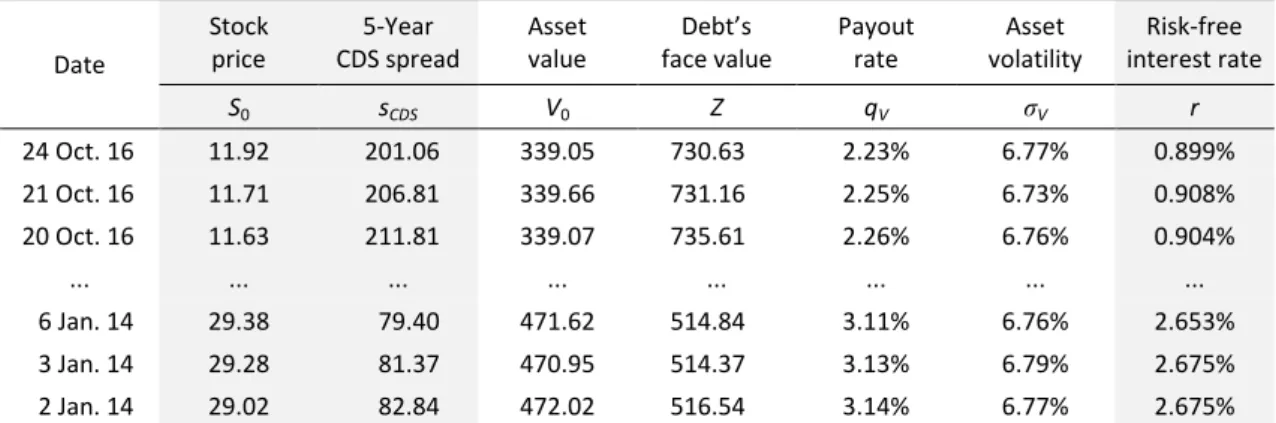
In order to estimate the input data of the PDSM, we used the daily quotes of Deutsche Bank’s common stock and CDS spreads for the period 2 January 2014 - 24 October 2016. The sample period is the same as that used by Moody’s ([19]) in one of its research papers. This makes it possible to compare the probability of default measured by the PDSM with the ex-pected default frequencies (EDFs) computed by Moody’s.
Some PDSM point estimates (V0, Z, qV, σV) are reported in Table 5. They make it possible
to ensure the “perfect fit” between the Deutsche Bank’s actual stock quotes and CDS spreads (Figure 3) and the theoretical quotes given by the PDSM.9
The estimates have been obtained under the hypothesis that the risk-free interest rate is well approximated by the 50-year OIS zero rate. In addition, the estimation procedure took into account the deviations between the actual and the theoretical values of some “control variables”: the price of 30-day at the money calls, the stock’s dividend yield, the balance-sheet leverage (which may diverge substantially from the “actual” one if the firm uses derivatives in-tensively).
9 The theoretical value of stock is S0 ≡ (1 – θ) (V0 – Z + P), where P ≡ (Z – Vb) pb, while Vb and pb are
giv-en, respectively, by Equations (1) and (2). The theoretical value of the CDS spread has been comput-ed by Equation (27) in Barone ([3], p. 12).
Table 5 Deutsche Bank: estimating PDSM inputs.
Date
Stock
price CDS spread 5-Year Asset value face value Debt’s Payout rate volatility Asset interest rate Risk-free
S0 sCDS V0 Z qV σV r 24 Oct. 16 11.92 201.06 339.05 730.63 2.23% 6.77% 0.899% 21 Oct. 16 11.71 206.81 339.66 731.16 2.25% 6.73% 0.908% 20 Oct. 16 11.63 211.81 339.07 735.61 2.26% 6.76% 0.904% ... ... ... ... ... ... ... ... 6 Jan. 14 29.38 79.40 471.62 514.84 3.11% 6.76% 2.653% 3 Jan. 14 29.28 81.37 470.95 514.37 3.13% 6.79% 2.675% 2 Jan. 14 29.02 82.84 472.02 516.54 3.14% 6.77% 2.675%
Note: θ = 29.58% (in 2014), 29.65% (in 2015), 29.72% (in 2016-7), based on KPMG data; α = 21.7% ([7]).
Figure 3 Deutsche Bank: stock prices and CDS spreads.
50 100 150 200 250 300 10 15 20 25 30 35
Jan-14 May-14 Sep-14 Jan-15 May-15 Sep-15 Jan-16 May-16 Sep-16
CD S sp re ad (b p) St oc k pr ice ( €) Stock price CDS spread
§5 A Firm-level Application: the Deutsche Bank Case. 13
According to the Moody’s research paper referred to above ([19], p. 1): “In January [2016 − Ed.] the bank reported its first full-year loss since the financial crisis. This exemplifies banks’ current difficulties, with low interest rates limiting their ability to generate profits from deposits, loans, and other market services. Deutsche Bank’s losses included €5.2 billion in pro-visions for fines and lawsuits. The firm’s one-year EDF measure increased from 1.05% in Janu-ary to its all-time high of 2.85% on FebruJanu-ary 9. ... Deutsche Bank’s current [25 October 2016 −
Ed.] one-year EDF measure maps to an EDF implied rating of B2, suggesting it is non-investment grade with a relatively high chance of default.”
The EDF, acronym of expected default frequency, has been obtained by mapping from the distance to default (DD). Technically, the risk-neutral measure (DD) has been transformed into a “real” measure (EDF). See Moody’s ([18], pp. 15-22).
As shown in Figure 4a, the 1-year EDF reaches a 2.85% peak shortly after the an-nouncement of the 2015 balance-sheet loss, released on 20 January 2016 by the Co-CEO of
(a)
(b) Source: Moody’s ([19], Figure 5, p. 5) and our estimates of Q.
Deutsche Bank, John Cryan. Comparison of Figure 4a and Figure 4b shows that the spread be-tween the 5-year EDFs and the 1-year EDFs is about 1 percentage point.10
In both figures, the dotted lines are the PDSM estimates of the “actual” or “real” default probabilities, Q*(T). As in the EDF case, these probabilities have been obtained by applying a mapping procedure. We assumed a linear relationship between real probabilities, Q*(T), and
risk-neutral probabilities,Q(T):
Q*(T) = λ0 + λ1 Q(T). (18)
In particular, we set λ0 = 0.01; λ1 = 1.11 for T = 1 and λ0 = 0; λ1 = 1 for T = 5.
The patterns of the EDFs and Q* in Figure 4 are reasonably similar, for both T = 1 and
T = 5. However, the value of the parameter λ0 for the case T = 1 highlights one of the limits of the diffusive-type models for V (the Merton model included). We had to set λ0 = 0.01 in order to have Q*(1) significantly different from zero. Likely, a jump-diffusive model would be more in
line with the real world, but at the cost of a much greater mathematical complexity.
We can now answer another question. Given our PDSM estimates, what would be the implied “market rating” of Deutsche Bank? As we have seen, “Deutsche Bank’s current [25 Oc-tober 2016 − Ed.] one-year EDF measure maps to an EDF implied rating of B2”. Now we will see that our risk indicators [σV, L, σS, Q(5), R, b, sb] map to a PDSM implied rating of Caa-C.
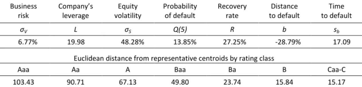
On 24 October 2016 the risk indicators for Deutsche Bank assumed the values reported in the upper part of Table 6. What is the “distance” between these indicators and those, by rating class, reported in Table 4? Which is the rating class most similar to Deutsche Bank’s?
Let di be the “Euclidean distance” of Deutsche Bank’s risk indicators, yj (j = 1, ..., 7), from
the corresponding indicators, xi,j, of the i th rating class (i = 1, ..., 7):
∑
= − = 7 1 2 ) ( j j i,j i y x d (19)The values of di have been reported in the lower part of Table 6 and in Figure 5. As can be
seen, the minimum distance (15.17) is the one from the Caa-C rating class. Therefore, this is the market rating estimated by the PDSM for Deutsche Bank.
The market rating estimated by the PDSM is a couple of notches lower than that (B2) es-timated by Moody’s (in the Moody’s scale there is only B3 before reaching the class Caa-C).
10 For EDF9, the term used in Figure 4, is meant the 9th generation of EDF, introduced in 2015 ([18]).
Table 6 Deutsche Bank: risk’s indicators (24 October 2016).
Business
risk Company’s leverage volatility Equity Probability of default Recovery rate to default Distance to default Time
σV L σS Q(5) R b sb
6.77% 19.98 48.28% 13.85% 27.25% -28.79% 17.09
Euclidean distance from representative centroids by rating class
Aaa Aa A Baa Ba B Caa-C
§6 Conclusions 15
6. Conclusions
In this paper, we outlined the general lines of a structural model that is based on the Leland model ([12]), but which differs from its assumptions about the tax regime.
In the model, which we called the Perpetual-Debt Structural Model (PDSM), the share-holders issue a perpetual fixed-rate bond and hold a perpetual American put option that al-lows them to declare the state of insolvency at any time.
The shareholders define ex-ante the default point in order to maximize the current value of the shares and to avoid it becoming negative.
The PDSM does not compete with the scoring models for the credit risk assessment of small and medium-sized companies, but can be effectively used by the risk management func-tions of financial institufunc-tions to monitor the “health” of large companies, listed on the stock exchange. Our theoretical framework plays a role similar to Moody’s KMV well-known model.
The main purpose of this paper was to carry out a first empirical test of the model, based on historically observed default rates, before making a more extensive test based on market prices.
To estimate the model, we minimized the sum of squared errors between actual and theoretical default rates. The coefficient of determination, R2, was 99.07%, indicating that the PDSM is sufficiently flexible to accurately explain the default rates historically observed by Moody’s.
The risk indicators obtained (Table 4) confirm the fact that firms with worse ratings are characterized by higher levels of leverage, business risk and equity volatility. Moreover, as the rating worsens, the default probability increases while the recovery rate, the distance to de-fault and the time to dede-fault decrease.
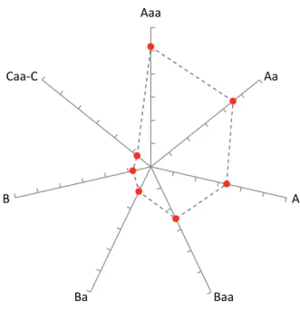
Figure 5 Deutsche Bank’s implied rating: distance from centroids (24 October 2016). Aaa Aa A Baa Ba B Caa-C
The paper also contains a firm-level application: the Deutsche Bank case. The PDSM’s input data were estimated to ensure the perfect fit of Deutsche Bank’s shares and CDS spreads, using stock option prices, dividend yields and balance-sheet leverage as control varia-bles.
The sample period used for the estimates was chosen to coincide with that used by Moody’s in one of its research papers ([19]). Therefore, it was possible to compare the proba-bilities of default measured by the PDSM with the expected default frequencies (EDFs) calcu-lated by Moody’s: the evolution of the two variables in the sample period is reasonably similar (Figure 4).
Finally, the risk indicators estimated by the PDSM for Deutsche Bank (business risk 6.77%, leverage 19.98, equity volatility 48.28%, 5-year default probability 13.85%, recovery rate 27.25%, distance to default −28.79%, time to default 17.09 years) were compared with the “typical” values of the rating classes to determine, based on their similarity, the “market rating” at the end of the sample period (October 24th, 2016). The market rating estimated by the PDSM (Caa-C) is lower, by a couple of notches, than the rating (B2) estimated by Moody’s.
References 17
References
[1] BARONE, G., “The Many Facets of Risk,” Working Paper, pp. 1-10, November 2004
[2] BARONE, G., “Equity Options and Bond Options in the Leland Model,” pp. 1-44, March 2011
(SSRN-id1779303.pdf).
[3] BARONE, G., “Equity Options, Credit Default Swaps and Leverage: A Simple
Stochastic-Volatility Model for Equity and Credit Derivatives”, May 2011 (see SSRN-id1826019.pdf). [4] BARONE, G., “An Equity-Based Credit Risk Model,” in Jonathan A. Batten and Niklas Wagner
(Eds.), Derivative Securities Pricing and Modelling. Bingley, UK: Emerald, vol. 94, pp. 351-378, July 2012.
[5] BARONE, G., “European Compound Options Written on Perpetual American Options,”
Jour-nal of Derivatives, Spring 2013, Vol. 21, No. 1, pp. 61-74.
[6] BLACK, F., and SCHOLES, M., “The Pricing of Options and Corporate Liabilities,” Journal of
Po-litical Economy, Vol. 81, No. 3, pp. 637-654, May-June 1973.
[7] DAVYDENKO, S. A., STREBULAEV, I. A., and ZHAO, X.,”A Market-Based Study of the Cost of
De-fault,” Review of Financial Studies, Vol. 25, no. 10, pp. 2959-99, 2012.
[8] FORSSBÆCK, J., and VILHELMSSON, A., “Predicting Default - Merton vs Leland,” Working
Pa-per, February 9, 2017 (SSRN-id2914545.pdf).
[9] HAMILTON, D. T., and CANTOR, R., “Measuring Corporate Default Rates,” Moody’s Investors
Service, pp. 1-16, November 2006.
[10] KALEMLI-OZCAN, S., SORENSEN, B, YESILTAS, S., “Leverage Across Firms, Banks and Countries,”
Journal of International Economics, Vol. 88, No. 2, pp. 284-298, November 2012.
[11] KASSOUF, S. T., “Stock Price Random Walks: Some Supporting Evidence,” Review of
Eco-nomics and Statistics, Vol. 50, No. 2, pp. 275-8, May 1968.
[12] LELAND, H., “Corporate Debt Value, Bond Covenants, and Optimal Capital Structure,”
Jour-nal of Finance, 49 (4), pp. 1213-52, September 1994.
[13] MERTON, R. C., “Theory of Rational Option Pricing,” Bell Journal of Economics and
Man-agement Science, Vol. 4, No. 1, pp. 141-183, Spring, 1973.
[14] MERTON, R. C., “On the Pricing of Corporate Debt: The Risk Structure of Interest Rates,”
The Journal of Finance, Vol. 29, No. 2, pp. 449-470, May, 1974.
[15] MODIGLIANI, F., and COHN, R. A., “Inflation, Rational Valuation and the Market,” Financial
Analysts Journal, Vol. 35, No. 2, pp. 24-44, March-April 1979.
[16] MOODY’S, “Corporate Default and Recovery Rates, 1920-2006,” pp. 1-48, February 2007.
[17] MOODY’S, “Corporate Default and Recovery Rates, 1920 - 2010,” pp. 1-66, February 28,
2011.
[18] MOODY’S, “Credit Risk Modeling of Public Firms: EDF9,” White Paper, 2015.
[19] MOODY’S, “Deutsche Bank’s Adversity Lifts its Probability of Default,” Moody’s, pp. 1-12,
25 October 2016.
[20] RUBINSTEIN, Mark, A History of the Theory of Investment – My Annotated Bibliography,
Ho-boken, NJ: John Wiley & Sons, pp. 1-370, 2006.
[21] U.S. DEPARTMENT OF SOCIAL SECURITY, Actuarial Life Table, www.ssa.gov/oact/STATS/table