AdWords Bid Optimisation
M
ASTER
T
HESIS
B
USINESS
M
ATHEMATICS
& I
NFORMATICS
VU UNIVERSITYAMSTERDAM
by Kevin Duijndam
AdWords Bid Optimisation
Author:
Kevin D
UIJNDAMSupervisors:
Dr. Wojtek K
OWALCZYK(VU)
Drs. Martijn O
NDERWATER(VU)
Drs. Eric J
ONKER(KLM)
Preface
The Master program Business Mathematics & Informatics at the VU Univer-sity Amsterdam is concluded by an internship. My internship took place at the Decision Support department of KLM Royal Dutch Airlines. In this report, the results of this internship are presented.
I would first like to thank my supervisor, Wojtek Kowalczyk, for his support throughout this internship. The good and practical ideas he always had were really helpful in concluding this internship. Also I would like to thank Martijn Onderwater, for all the help in finishing this project. Both his help in practical matters and his comments on the report have helped a lot in improving this report.
Finally, I would also like to thank my colleagues at KLM Decision Support for their help and support. Especially Eric Jonker for the, mostly technical, advise and knowledge of the Google AdWords system.
In this report, some parts are confidential. They are either shown like this: , or they are left out completely and replaced by ’Confidential’. Kevin Duijndam
Management Summary
Companies spend more and more money on online advertising and a very important part of most companies’ advertising campaigns is paid search. An important aspect of advertising through paid search is how much one is will-ing to pay for a position on the results page. Generally these positions are auc-tioned per search phrase and therefore advertisers have to set bids per search phrase.
To get a better understanding of the way this auction works, first the current situation is analysed. It is shown that being displayed on the first position almost doubles the chances of being clicked.
Using this analysis, keywords can be clustered together to try to discern dis-tinct groups of keywords. It is shown that there is a small group of keywords that have very different statistics compared to the other keywords. These key-words are either a lot more effective (keykey-words like ) or a lot more ex-pensive but not effective at all (keywords like ). There are also a lot of keywords that are never, or almost never, clicked or viewed. Two other groups of keywords were found with more and less active keywords.
To optimise bidding on keywords a combination of a knapsack model and a Markov decision process model is proposed that is able to adjust its bid during the budget period. This results in an improvement in the spending on adver-tisements via paid search and is shown to outperform a fixed bid consistently. An increase in performance of up to 10% is observed in simulations.
Contents
1 Introduction 2
1.1 Business Mathematics and Informatics . . . 2
1.2 KLM . . . 2 1.3 The problem . . . 3 1.4 Report Outline . . . 4 1.5 Goal . . . 4 2 Google AdWords 5 2.1 History . . . 5 2.2 Auction . . . 6 2.3 Common practice . . . 8 3 Data Analysis 9 4 Clustering 10 5 Modeling the auction 11 5.1 The knapsack problem . . . 11
5.2 The model . . . 12
5.3 The online knapsack problem . . . 13
5.4 Single-Slot Auction . . . 14
5.5 Multiple-slot auctions . . . 15
6 The bidding process as a Markov Decision Process 17 6.1 Markov Decision Processes . . . 17
6.2 The model . . . 19
7 Results 22 7.1 The Knapsack Approach . . . 22
7.1.1 The performance of the algorithm . . . 22
7.1.2 Using the algorithm on real data . . . 27
7.1.3 Optimising the algorithm . . . 28
7.1.4 Conclusion . . . 30
7.2 The Markov decision process approach . . . 31
iv CONTENTS
7.2.2 Using the algorithm on real data . . . 33 7.3 Comparing the two methods . . . 33 7.4 Combining the two methods . . . 35
8 Conclusion 37
8.1 The adwords . . . 37 8.2 The auction . . . 37 8.3 Further work . . . 38
A Proof of optimality 40
A.1 Single-slot case proof . . . 40 A.1.1 Remark: . . . 41 A.2 Multi-slot case . . . 41
List of Figures
6.1 A graphical model of the used Markov chain . . . 18 7.1 The computed bid for a certain keyword as a function of the
budget that is left . . . 23 7.2 Histograms comparing the knapsack- and dummy-bidder in
sce-nario 1 . . . 24 7.3 Histograms comparing the knapsack- and dummybidder in
sce-nario 4 . . . 26 7.4 Barcharts with the results of the two strategies of all simulations 27 7.5 The epsilon and upperbound from generation to generation . . 29 7.6 The computation time for a growing number of keywords . . . . 31 7.7 The expected optimal value (or return) per user versus the
bud-get that is allocated per user . . . 32 7.8 A comparison of the computation times of the two approaches . 34 7.9 The computation times of the partitioned approach . . . 35
List of Tables
7.1 Statistics from the simulation with a dummy bidder bidding 0.2, scenario 1 . . . 24 7.2 Statistics from the simulation with a dummy bidder bidding
uni-form between 0.2 and 10, scenario 2 . . . 25 7.3 Statistics from the simulation with a dummy bidder bidding
uni-formly between 0.2 and 3, scenario 3 . . . 25 7.4 Statistics from the simulation with a dummy bidder bidding 1.4,
scenario 4 . . . 26 7.5 Statistics from the simulation with two knapsack-bidders . . . . 27 7.6 Statistics from the simulation with the optimised knapsack-bidder 29
Chapter 1
Introduction
1.1
Business Mathematics and Informatics
Business Mathematics & Informatics1is a multidisciplinary programme
com-bining mathematics and computer science with business management knowl-edge. These factors are aimed at improving business processes through mathe-matical optimisation. Since BMI tries to be as practical as possible, it is required to finish the study by doing an external research project. This report is the end result of this research.
1.2
KLM
KLM stands for ’Koninklijke Luchtvaartmaatschappij’ or Royal Dutch Air-lines. It is the oldest Dutch airline in existence with a substantial interconti-nental network, albeit no longer independent as of its merger with AirFrance, founded on 7 October 1919 and one of the largest in the world after the merger. Its first commercial flight was carried out on 17 May 1920 between London and Amsterdam [6]. On 1 October 1924 KLM commenced its service to Batavia in the Dutch-Indies, the longest scheduled flight service before the second world war [7]. In 1946 KLM was the first European airline to commence service to the United States. Since 1993 all flights between Europe and the US are operated under a joint venture agremeent, first between KLM and its partner Northwest Airlines, and later with Delta Airlines. On 5 May 2004 KLM merged with Air France to become Air France-KLM. Currently, KLM has well over a hundred airplanes, excluding subsidiaries and daughters, flying to about 140 different destinations worldwide, with about 33,000 people employed. KLM is also a founding member of Skyteam, a global airline alliance with 13 members2that provides access to a global network with over 12,500 daily flights to 898
des-1From now on, BMI. 2In February 2011
3 Introduction
tinations in 169 different countries. Since the joint-venture with Northwest Airlines, daily cross-Atlantic frequency has risen tremendously with currently almost 250 daily trans-Atlantic flights.
KLM has various daughter companies and subsidiaries:
• Martinair (100%) • KLM Cityhopper (100%) • Transavia.com (100%) • KLM Cargo (100%) • EPCOR3(100%) • KLM Flight Academy (100%) • Cygnific BV4(100%) • Kenya Airways (26%) • HSA5(10%)
1.3
The problem
Besides the main business of transporting people and goods, KLM also needs to advertise its tickets to potential customers. Ever since the rise of the Internet, more and more advertisements are being placed on the web. Besides placing normal advertisements like for instance banners on a website, another reward-ing possibility is that of advertisreward-ing on search engines. This is very effective as people are already searching for something and if an advertisement is corre-lated to their search, they are a lot more likely to be interested in the advertise-ment. Therefore, advertising via search can be very effective. KLM places a lot of advertisements at Google and logically, KLM needs to pay Google for this. Google auctions advertisement places and for every advertisement a bid has to be placed. If a bid is too low, an advertisement will not be displayed, but on the other hand if a bid is too high, one might pay too much. The problem is to find the best bids for the advertisements in such a way that the advertisements are as effective as possible.
3European Pneumatic Component Overhaul & Repair is a repair and overhaul facility for en-vironmental control system components, engine starters, leading edge flap drive units, air driven pumps and other pneumatic components installed in all models of large commercial aircraft.
4Cygnific is an international, multi-channel, sales & service center for travel related services. 5High Speed Alliance is an alliance between NS (the Dutch railway company) (90%) and KLM (10%) and it is a company that runs high-speed train services in Holland.
4 Introduction
1.4
Report Outline
In this report I will investigate the problem of advertising on the Internet via paid search channels, and more specifically, via Google AdWords. First I will give a brief explanation of what Google Adwords precisely is and why it is relevant to investigate this in chapter 2. Then, I will continue with a short investigation of what exactly can be said about these advertisements. For in-stance, how often are the advertisements viewed per day? And how often do people click on them? Is there a large spread in how often people book after they have clicked? This can all be found in chapter 3. I will continue with clustering the advertisements into groups of advertisements, as investigating every single advertisement is neither possible nor very rewarding. How this is done is explained in chapter 4. After this a model for the auction is proposed which allows for computations in chapter 5 A completely different approach is described in chapter 6. Results obtained by both models can be found in chap-ter 7, where also a hybrid model is proposed that uses the strengths of both of the proposed models.
1.5
Goal
The goal of this research is to optimise KLM’s spending on Google AdWords. Optimising can be done in several ways: either by spending less money while keeping the same number of bookings, or by spending the same amount, while getting more bookings through the advertisements. Even something in-between is possible, where the number of bookings increase and the spendings decrease. Since the advertisements are displayed based on an auction system that re-quires bids, the goal is to optimise KLM’s biddings on this auction.
Chapter 2
Google AdWords
Google AdWords is the service Google offers to companies to advertise on the search channel of Google, the well-known ’google.com’. When a customer searches on Google for ’klm’, the first item that is displayed is an advertisement of KLM. Underneath this advertisement are the actual search results, in which KLM might appear as well.
2.1
History
Around the year 2000 search engines on the Internet became a source where one could properly find information. Up until then, a lot of unrelated websites could also pop up on a search. Google was one of the first to get good search results and it is still the most used search engine on the web [3] with about 65% of the people searching something using Google. Google started its AdWords program in 2000 to generate more revenue [4] and this set the standard for search related advertisement. The Google AdWords program was the first to combine a cost per click with a quality score. Before AdWords, search engines generally placed the advertiser that was willing to pay the most per click on the first spot, expecting that this would maximise their income. With AdWords, Google changed this in a very smart way. Instead of displaying the advertiser that was willing to pay $5 per click, but only getting clicked 1% of the time, Google preferred the advertiser that was only willing to pay $1 per click, but getting clicked 10% of the time. In that way, search results are more relevant to the user, companies that are more relevant need to pay less per click and Google earns more.
Paid search is now the biggest revenue driver for most search engines. Google in 2009 for example generated a revenue of about $22 billion worldwide in paid search, with 37 billion clicks at a $0.60 average cost per click [3]. Advertisers are also spending more and more money on paid search, spending almost half of their online advertisement budget on search engine marketing - $11 billion
6 Google AdWords
out of $22 billion total online advertising - with most of this $11 billion being paid search [5].
2.2
Auction
The way Google displays its advertisements makes it necessary to have an ordering, since the results are shown in a list. To determine an ordering of the advertisements, Google uses an auction-based system [8]. When an advertiser wants his advertisements to be displayed at Google, besides making the adver-tisement itself, the advertiser also needs to determine a maximum cost per click for his advertisement. Together with a predetermined budget this determines whether the advertisement is shown.
However, Google does not only take money into account. To remain an at-tractive platform for searching, it needs to take relevance for searchers into account as well. Therefore, instead of just basing the ordering on the cost-per-click someone is willing to offer, Google also tries to determine a ’quality score’ for the webpage the advertisement links to. Google does not disclose in what way this ’quality score’ is determined, but it should take relevance into account for instance. Then the ordering of the advertisements is done based on the fol-lowing simple formula:CP Cbid·QualityScore=EndResult. Then, these end results are sorted in a scale from high to low and the advertisement with the highest ranking is displayed first.
It does not seem entirely fair to have to pay a certain price, even if you could have paid less to be displayed on the same place. Therefore, Google does not charge you the full amount of your bid per click. It looks at the advertisement placed directly underneath and then charges you exactly what is required to still be displayed at your current position. So if advertisement X bids 1 and has a quality score of 10, it gets an end result of 10. If advertisement Y bids 2 but has a quality score of 2, it gets an end result of 4. Advertiser X will now not have to pay the 1 it bid, instead, it has to pay exactly what is required to remain on top of Y, so it needs to keep its end result above 4. This means X will only have to pay 0.41 instead of the 1 of its bid.
This auction system, in which you do not have to pay what you bid yourself, but what the person directly below you bids is called a second price auction, and it has some surprising features. One would expect that this bidding system is negative for the auctioneer, as the bidders are required to pay less. Perhaps surprisingly, this is not the case. The expected income for the auctioneer is exactly equal to what it would get using a first price auction (so an auction in which the bidder just has to pay its bid)[1]. This might sound counter-intuitive, however, it can be shown that in such an auction, it is optimal for a bidder to bid the amount exactly equal to what it is worth to him. Since it is not known
7 Google AdWords
what others are willing to bid, and since the winner of the bid only pays the second price, it is optimal to bid exactly what it is worth to him. If he wins the auction, he pays just as much as when he had tried to be smart and bid less, but if he tries to be smart and bid less, his chances of not winning the auction increase. Therefore, it is optimal to bid as much as it is worth to the bidder. And because it is optimal for every person that bids to bid the value it is worth to him, the auctioneer can expect to get the optimal value.
However, this explanation does not take everything into account. The as-sumption was that there is only one thing to auction, but Google auctions mul-tiple places. This is the case of the so-called ’Generalized Second Price Auc-tion’. In this type of auction, it is not optimal anymore to bid the value the auctioned object represents to you [2]. Suppose for instance there are three advertisers, with values per click of $10, $4 and $2, and two positions to be auc-tioned. Now the click-through rates of these two positions are almost the same: the first position receives 200 clicks per day and the second position gets 199 clicks per day. If all bidders bid truthfully, then advertiser 1s payoff is equal to
($10−$4)·200 = $1200. If instead, he bids only $3 per clicks, he will get the second position, and his payoff will be equal to($10−$2)·199 = $1592>$1200.
This complicates the analysis of this auction system. It is actually even prov-able that GSP in general does not have an equilibrium in dominant strategies [2]. But it can be shown that if the GSP is modeled as a Generalized English Auction it does have a unique equilibrium. A Generalized English Auction is a standard English auction, so one in which the prize goes up as long as bid-ders are willing to bid. Think for instance of a regular art auction, but with the addition that there are more versions of the same thing to auction, like the places for an advertisement. This equilibrium has some notable properties and the most interesting of them is that the bid functions have explicit analytical formulas. These formulas do not depend on bidders’ beliefs about each others’ type, the outcome of the auction only depends on the realizations of bidders’ values. One very heavy assumption in this proof is that all bidders have com-plete information, so that they know what other players have been bidding up until the point where they have to make their decision, and what the value per click is for other players. When keeping this in mind, it is shown [2] that in the unique perfect Bayesian equilibrium of the generalized English auction with strategies continuous insk, an advertiser with valueskdrops out at price
pk(i, h, sk) =sk−ααi
i−1(sk−bi+1).
with
pk(i, h, sk) The price at which a player drops out
bi Thei-th bid
αi The click through rate at position i
sk The value per click of advertiser k
8 Google AdWords
h The history of prices at which previous advertisers have dropped out
The intuition behind this is that withiplayers remaining and the next bid equal tobi+1, it is a dominated strategy for a player with valuesto drop out before
the pricepreaches the level at which he is indifferent between getting position
iand payingbi+1per click and getting positioni−1and payingpper click.
2.3
Common practice
To give a better understanding of this process in practice, the common prac-tice is explained here. Suppose a company wants to advertise on Google Ad-Words, first, a set of keywords will have to be determined on which the com-pany wants to be displayed. This means that if someone searches for one of the keywords that was set by the company, an advertisement from the company can be displayed. After determining this set of keyword possibly thousands -advertisements will need to be made that are linked to the keywords. One ad-vertisement can be linked to a lot of keywords, as keywords can be very similar. To structure all these keywords and advertisement, campaigns can be made in which keywords and advertisements can be grouped together.
Now for every keyword, a bid will have to be set at the Google servers, that is the maximum price the company is willing to pay for someone clicking on this keyword. So if there are thousands of keywords, thousands of bids will have to be set. Besides the bid, a budget will have to be set as well, which is generally set at campaign level. The budget ensures that never more than what is set is spent. If the budget runs out, advertisements are no longer displayed and thus no cost can be incurred. Because of the high number of keywords, general practice is to set these bids once, and then leave them the same for perhaps months.
The company will want to know whether it is doing well with its advertising campaign, so some feedback is given from Google. Daily reports are stored on the Google servers that show how many times it was viewed, how many clicks and conversions came from a keyword, what the cost was, and on what position it was shown on average. These reports can be downloaded, at a price. Effectiveness is generally measured by the average cost per click that is in-curred and the number of conversions that result from the campaign. Since information about other bidders is not available, it is hard to compare with other bidders.
Chapter 3
Data Analysis
Chapter 4
Clustering
Chapter 5
Modeling the auction
A lot of work has been done on modeling the bidding on keywords for ad-vertisement auctions (see for instance [13], [14] or [15]). Almost all the work models the choice of keywords as a stochastic knapsack problem, all recognis-ing that this is an online variant of the knapsack problem. Meanrecognis-ing that instead of knowing beforehand how well a choice will be, this can only be known af-ter the decision has been made. And also that there is usually more than one slot for the advertiser, so instead of picking or not picking an advertisement, another decision based on position needs to be made.
5.1
The knapsack problem
The knapsack problem is a classical problem in operations research. In its simplest form, it can be seen as the problem of filling a knapsack. The knapsack has a limited capacity, sayB. And in the knapsack various items can be put, where every item has a certain valuevi and a weightwi. Some items might
be worth more than others, but they can also have more weight than others. The problems is to fill this knapsack with as much value as possible, while still remaining below the capacity limitation. Usually this problem is studied as a 0-1 knapsack problem, so that every item either can be taken or not. Let
xi∈ {0,1}denote whether an item is put in the knapsack or not. The problem
is then defined as max i xivi such that X i xiwi≤B.
12 Modeling the auction
5.2
The model
For now, the model of [15] will be followed. First, a simplified model will be considered in which there is just one slot, one keyword and one advertiser. Two choices could be made in deciding in what way to advertise. Either by determining in what position an advertisement should be, or by specifying a bid directly. Determining in what position an advertisement should be might be a better approach, however this does require an extra mapping from posi-tion to bid and this is informaposi-tion that is not easily available. Therefore in this approach, a direct decision on the bid will be made. But first, the model itself should be specified. Suppose there areN+ 1bidders{0,1, . . . , N}interested in a single keyword. Bidder 0 is an omniscient advertiser and his expected value per click for this keyword isV. Bidder 0 has a budget ofB over time period
T, and he wants to maximise his profit over the time periodT. This budget is a hard constraint, meaning that once it is exhausted, the budget can not be refilled. Budget remaining at the end of periodT is forfeited.
Bidders all bid on the keyword and are allowed to change their bid at any time. When a query arrives at the search engine, the search engine allocatesS
slots to bidders as follows: It takes theShighest bids,b1≥b2≥b3 ≥ · · · ≥bS
and displays thes-th bidders advertisement in slots. If a user clicks on the ad in thes-th slot, the search engine charges thes-th bidder a pricebs+1, ifs < S
or a minimum feebmin. It is assumed each slot has a click-through rateα(s).
This value might change from advertiser to advertiser, but since we only focus on one advertiser, these valuesα(s)can be assumed to be constant (over the advertisers, not over the slots). So to summarise, each time an ad in slotsof an advertiser is clicked, he is charged a cost ofbs+1, he obtains an expected
revenue ofV and a profit ofV−bs+1. The timespan T is discretised into period
{1,2, . . . , T}such that within a time period no advertiser changes his bid. If we would know bids of all the advertisers at each time period, the best bidding strategy corresponds to solving a knapsack problem. Suppose there is only one ad slot, soS = 1andα(s) =α. At each time periodt, letb(t)be the maximum bid on the keyword among bidders1toN. The omniscient bidder knows all the bids{b(t)}T
t=1. To maximize his profit, he should bid higher
thanb(t)at those times that give him maximum profit and keep his total cost within budget. Winning at timetcosts himw(t) = b(t)X(t)αand earns him
v(t) = (V −b(t))X(t)α, whereX(t)is the expected number of queries at time periodt1, andX(t)αis then the expected number of clicks att. So he should choose timesΘ ⊆T to maximisev(Θ) = P
t∈Θv(t)satisfying the constraint w(Θ) =P
t∈Θw(t)≤B. This is a standard instance of the classic 0/1 knapsack
problem. However, for the bidding optimisation problem, items arrive in an online fashion, instead of being able to decide after knowing everything in the end. At each time periodt, a bidder has to decide either overbiddingb(t)or
13 Modeling the auction
not, without knowing the future. And furthermore, it is not possible to revoke past decisions. So keyword bidding optimisation corresponds to the online knapsack problem.
5.3
The online knapsack problem
In this case, the auction is considered with still one bidder, one slot and one keyword, however, the future in this case is not yet known. The knapsack lem is a classic problem in operations research. For the online knapsack prob-lem, it is shown that in its most general case there can be no online algorithm that achieves any non-trivial competitive ratio. Here the competitive ratio is defined as the ratio of the value of the best online algorithm to that of the best offline algorithm [17]. However in this case two reasonable assumptions can be made which allow to develop an algorithm. These assumptions are: 1. Each item has a weight much smaller than the capacity of the knapsack, so
w(t)B, ∀t.
2. The value-to-weight ratio, or efficiency, of each item is both lower and upper bounded, soL≤wv((tt)) ≤U, ∀t.
Recall thatw(t) =b(t)X(t)αandv(t) = (V −b(t))X(t)α. The assumption that
w(t) B,∀t is justified because the budget is usually much larger than the money spent in small time periods as the bids are relatively small. The second assumption is a little bit harder to justify. Since wv((tt)) =
V
b(t) −1, it suffices to
setU ≡ V
bmin−1. An obvious choice for the lower bound might be0, however, since we want to use theseU andLin formulas, settingLto0is not possible. To get a good lower boundL, notice that ifb(t)is close toV, little is lost when not bidding at those time intervals. So if we only bid whenb(t) ≤ V
1+ε for
some fixedε, the maximum amount of profit lost from not bidding in these time periods isεB. To see this, note that ifV ≈b(t),v(t)≈0. And ifb(t)≤ V
1+ε,
we can not bid on items that areεclose toV, which results in a loss of at most
εB, since the entire budgetB would be spent on bidding on these items, with a return ofεper item. Ifεis small, then the profit loss can be negligible. So we can setL=εand ignore all items with efficiency smaller thanε. The efficiency of an item is defined as wv((tt)).
The input sequence consists of a knapsack of capacityB and a stream ofT
items having values and weightsv(t), w(t). The goal is to choose these items in an online fashion, so decisions need to be made when items come along so as to maximise the total value. Define the competitive ratioγof an algorithm
Aasγif for any input sequenceσ, we haveOP T(σ)≤γ· A(σ). HereA(σ)is the expected value obtained byAgivenσ, andOP T(σ)is the maximum value that can be obtained by any offline algorithm with the knowledge ofσ. The algorithm described here is competitive with ratioγ= ln(UL) + 1, see [15].
14 Modeling the auction
LetΨ(z) = (U eL )z(U
e). At timet, letz(t)be the fraction of capacity filled, so
z(t)∈[0,1], pick - or in the auction contest, bid on - elementtiffwv((tt))≥Ψ(z(t)).
Note that forz ∈[0, c]wherec≡ 1
1+ln(U/L),Ψ(z)≤L, thus the algorithm will
pick all items until a fractionc of the knapsack is filled. We can assume that
Ψ(z) =Lforz∈[0, c]. Whenz= 1,Ψ(z) =U, and sinceΨis strictly increasing, the algorithm will never overfill the knapsack. In short,
Ψ(z) = L ifz∈[0, c] U ifz= 1 U e L z U e otherwise. (5.1)
For a proof, see appendix A.
5.4
Single-Slot Auction
Now we have an algorithm for the online knapsack problem, but this does not easily translate to a strategy for bidding strategies. Again, a case with one advertisement and one slot is considered, however this time we have an opponent and we compute what to bid. The bidding optimisation objective can be to either maximise profit or revenue. Both strategies will be considered here, the only difference is in the parameter settings.
For profit maximisation, recall that outbiddingb(t)at time t gives an effi-ciency of wv((tt)) = bV(t) −1while for revenue maximisation it is V
b(t). Thus, the
parametersU andLfor revenue maximisation areUr:=bV
min andLr:= 1. For profit maximisation this isUp:=Ur−1, butLpcould be0. To circumvent this,
the parameterεis introduced and we bid only when the efficiency is greater thanε. ThenLp=ε, but this leads to an additive loss over the optimal value.
The strategies are derived from the algorithms introduced before. So we should only bid when the efficiency is higher than the threshold. And since the thresholds in the algorithms only depend on the fraction of the knapsack filled, the strategies only depend on the remaining budget. The strategies can be stated as follows:
• For the profit-maximisation case, letΨ(z) = (Upe
ε ) z ε
e. At time t, if the
fraction of the budget spent isz(t), then bidb0(t) =1+Ψ(Vz(t)).
• For the revenue-maximisation case, letΨ(z) = (Ure)z
1
e . At time
t, if the fraction of the budget spent isz(t), then bidb0(t) =1+Ψ(Vz(t)).
Note that both strategies only need the fraction of the budget spent and there-fore need no other knowledge of the auction. Denote the profit and revenue
15 Modeling the auction
earned by the above strategies byP rof itand Revenue,OP Tpand OP Tr
de-note the optimal values that can be obtained. For anyε >0, we haveOP Tp ≤
εB+ lne(V−bmin)
εbmin
·P rof it. This follows from what was mentioned earlier, thatOP T(σ) ≤ A(σ) ln(U
L) + 1
for this algorithm and the fact that all items with efficiency≤εhave total value at mostεB. This also suggests that different values ofεalso give different guarantees forP rof it. So we can actually treatL
as a tunable parameter and thus improve the efficiency of the algorithm. We also getOP Tr≤ln
eV bmin
·Revenue. This also follows fromOP T(σ)≤ A(σ) ln(UL) + 1
, settingL = 1. This is valid if the budget is not very large. And in practice, when wanting to maximise revenue, rarely you would still want to buy unprofitable keyword positions.
5.5
Multiple-slot auctions
In practice however, there are no single-slot auctions, but multiple-slot auc-tions. Therefore in this section the case with one advertisement, multiple slots, and multiple bidders is considered. So the previous formulas need to be gener-alised to the multi-slot case. This requires changes in both the online knapsack problem, as this has now become a online multiple-choice knapsack problem2,
and the translation to the algorithm.
For the Online-MCKP, at each time period, at most one item has to be chosen from an item setNt. The goal is again to maximise the total value of the items
chosen.
LetΨ(z) = (U eL)z Le. At timet, letz(t)denote the fraction of capacity filled and
Bthe budget,Et=
n
s|vs(t)
ws(t) ≥Ψ(z(t))
o
, pick elements∈Etwith maximum
vs(t). This algorithm has a competitive ratio ofln(UL) + 2. For a proof, see A.2.
But this is only an algorithm for the Online-MCKP, what is needed is again a strategy for bidding. Again, both profit-maximisation and revenue-maximisation situations are considered. At each time period, the bidder has to decide which bidders he should outbid. The algorithm suggests to bid so as to get a maxi-mum profit or revenue, while having a minimaxi-mum efficiency. However, bidding to get maximum profits requires knowledge of other bidders bids, and these are generally not available. On the other hand, assuming that higher slots re-sult in higher click-through rates (as found in section??), bidding higher would result in higher revenue. Therefore, an algorithm for the revenue maximisation objective, is easier.
16 Modeling the auction
In the profit maximisation case, the parameters are the same as in the single-slot auction case. The algorithm is then as follows:
Fixε > 0. Let Ψ(z) = (U eε )z ε
e. At timet, letz(t)be the fraction of the
bud-get spent,Et =
n
s|bs(t) ≤ 1+Ψ(Vz(t))
o
, bidbs(t)wheres = arg maxs∈Et(V −
bs(t))α(s).
This bidding strategy requires knowing the bidsbs(t), the other players bids,
andα(s). This bidding strategy also has a performance guarantee, namely,
OP Tp≤εB+ ln( V εbmin ) + 2 ·P rof it, ∀ε >0. (5.2)
For the revenue maximisation case, we can actually find the slotsin timetto maximise the revenue. This is true, because the revenue obtained on bidding
bs(t)isV X(t)α(s). And since the assumption was made thatα(s)is a
decreas-ing function, maximisdecreas-ingV X(t)α(s)is equivalent to minimisings. And since the efficiency condition imposes thatbs(t)≤ Ψ(zV(t)), our bid should be exactly
that. This bidding strategy has a performance guarantee of
OP Tr≤ ln( V bmin ) + 2 ·Revenue (5.3)
Chapter 6
The bidding process as a
Markov Decision Process
Besides seeing the problem of bidding on keywords as a stochastic knapsack variant, this problem can also be modeled using a Markov chain analysis. In this chapter this approach is used, mainly following the model of [18].
6.1
Markov Decision Processes
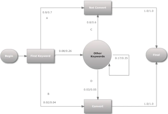
The problem of bidding on keywords is now viewed as a Markov decision process. This means that the mechanism behind the auction is viewed as a Markov chain, in which decisions can be made. Logically the decision in this case is whether to advertise or not, and if so, how much. The model we use here is one that is based on a user of the system, e.g. of someone that is search-ing at Google. This person is only seen as a user once he searches for somethsearch-ing that was advertised for. After this, various things can happen. If the bid was high enough, he gets to see the advertisement, otherwise he will not see it. If he does see the advertisement, he either clicks on it and buys something, or sees it, remembers it, but does not buy anything. If he did see the advertisement, he could either remember the advertisement and search for something else re-lated, and gets displayed another advertisement, or he abandons the search. Once again, when he sees something else related he could either click on it and buy something, remain searching or leave the system. This is visualised in figure 6.1.
In this picture, the user enters the model by searching for the first keyword. After that, if the decision was made not to advertise, he has a 0.9 chance of not converting and directly leaving the system (flow A), 0.08 of going to any of the other keywords and a 0.02 chance of directly converting (flow B). If on the other hand the decision was made to advertise, he has a 0.7 chance of not
18 The bidding process as a Markov Decision Process
Figure 6.1: A graphical model of the used Markov chain
converting and directly leaving the system (flow A), a 0.26 chance of going to another keyword, and a 0.04 chance of directly converting (flow B). After a user has either converted or not converted, all users move to the end of the system with probability 1. The other keywords are shown seperately, because this allows to model a carry-over effect. Note that if the user goes to another keyword, the probability of converting increases from 0.02 to 0.03 when not advertising (flow D). This is why the probabilities in flow A are larger than those in C and similarly the probabilities in flow D are larger than those in B; the carry-over effect.
The intuition behind the possibility of going from one keyword to another is that it is possible that a user first searches for a specific flight to get information about that flight. He then sees the KLM advertisement and does some more investigating. After his investigations, he decides he wants to fly with KLM
19 The bidding process as a Markov Decision Process
and then Googles for KLM to book a flight. This effect is called carry-over and is observed in other advertisement settings as well [19]. However, after the user has done his research and made the decision to either buy his ticket or not, the user is not searching for a flight anymore and therefore is no longer in the system.
6.2
The model
This MDP model is very different from the knapsack model. Instead of look-ing at keywords separately, all keywords are considered at once. This has the advantage of being able to model the previously mentioned effect of carry-over. LetX be the state-space representing possible user states. In accordance to figure 6.1 a statex ∈ X captures the last query the user has done within the system, in this case any search on a KLM keyword, or the decision to convert or not convert. For anyx∈X, letA(x)represent the possible actions - in this case advertisement levels, or what to bid - in statex. Furthermore, letc(x, a)≥ 0
denote the immediate cost of choosing actiona in statex, so this is actually what we need to pay if deciding to advertise. This relates to a constraint there is in the budget, let this budget be defined as B. Now letPxay denote the
probability of going from xtoy when choosing actiona. The initial flow of users to the system is defined asβ(x), which in this case translates to the first search query a user has. The problem is now to maximise the number of users that enter the convert state subject to the budget constraint. If we normaliseβ
to 1,βrepresents a probability measure which denotes the probability of a user searching for a certain keyword, and the budgetBrepresents a per-user budget. The problem can be seen as a Markov Decision Process by defining the reward function asr(x, a) ≡ V ifx = xc andr(x, a) ≡ 0otherwise. Since the final,
absorbing state was introduced, the optimisation problem is well-defined. For every distributionβof initial states and a policyu, there is a unique mea-sure on the space of trajectories that can be taken. LetPu
β denote this measure.
Then definepu
β(t;x;a) = Pβu(Xt =x;At = a)as the probability of observing
statexand advertising levelaat timetwhen following policyu. Intuitively this can be considered as the probability of being in a certain state when start-ing fromβ after time t. We can then define the total expected reward for a policyuas R(β, u) = ∞ X t=1 X X,A puβ(t;x;a)r(x, a) (6.1) and the total expected cost for a policy as
C(β, u) = ∞ X t=1 X X,A puβ(t;x;a)c(x, a). (6.2)
20 The bidding process as a Markov Decision Process
Now the optimisation problem is simply defined as
max
u∈U R(β, u)
s.t. C(β, u)≤B, (6.3)
whereUis the set of policies of interest. So choose a policy that maximizes the reward - and in this case this means, get as many people as possible to convert - while not spending more than the budget.
Of course, iterating over all possible policies at every possible time instance is impossible, as there are far too many possibilities. In accordance with [20], there are three classes of policies of interest:
• InMarkov policies,utdepends only onxt(and not on(xt−1, . . . , x0)), so
in this case users are targeted based only on their current state and the amount of time they have spent in the system.
• Instationary policies, a special case ofMarkov policies,utdoes not depend
ontbut only onx, so users are targeted only based on their current state.
• Instationary deterministic policies, a special case ofstationary policies, the action uis chosen deterministically, so in this case, all the users in the same state are targeted in the same way.
For this case, it is sufficient to restrict attention to Markov policies, as for any general policyu, there exists some Markov policyv such thatpu
β(t;·;·) ≡
pv
β(t;·;·). The proof for this can be found in [20]. Furthermore, letX0 = X \ {xf}, wherexf is the final absorbing state. An occupation measure is a ”visit
count” measure over the set of states and advertising levels(µ∈M(X0×A))
achievable by some Markov policyu:
µ(x, a) =
∞
X
t=1
puβ(t;x;a).
In short, this can be seen as the probability that a given user is in a state(x, a). Furthermore, in [20] it is also shown that in this case, a probability measure
ρcan be defined, which is equal to such an occupation measure and which follows ∀x∈X0 X y∈X0 X a∈A ρ(y, a)(δx(y)− Pyax) =β(x) (6.4) whereδx(y)is the standard delta-function.
21 The bidding process as a Markov Decision Process
Note that equation 6.4 is the basic ”conservation of flow” statement, so this can be interpreted as ”any measure satisfying the set of conservation of flow constraints is achievable with some stationary policy”. This means we only have to search for stationary policies and even better, we can look for the solu-tion in the form of an occupasolu-tion measure like thisρ. Then 6.3 can be translated to: max ρ X x∈X0 X a∈A r(x, a)ρ(x, a) (6.5) s.t. X x∈X0 X a∈A c(x, a)ρ(x, a) ≤B X y∈X0 X a∈A ρ(y, a)(δx(y)− Pyax) =β(x) ∀x∈X0 ρ(x, a) ≥0 ∀x∈X0, a∈A
Now ifρ∗is the optimal solution of 6.5, then the stationary policyu∗
choos-ing the advertischoos-ing level a with probability of Pρ∗(x,a)
bρ∗(x,b) is the optimal ran-domised stationary policy [18].
Chapter 7
Results
In this chapter, first the results for both the knapsack- and MDP approach will be discussed and after that a comparison of both approaches is made. It is more convenient to compare using generated data because then specific cases can be generated and compared, rather than a big mixture of cases in a full dataset.
7.1
The Knapsack Approach
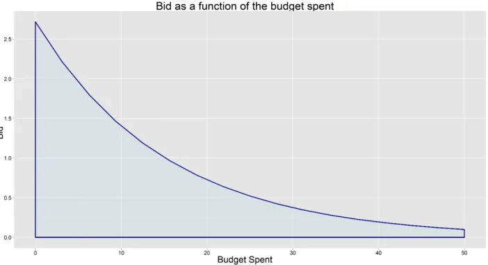
This approach computes bids as a function of the portion of budget that is left and the amount that the keyword is worth. For instance for the case that a keyword has a worth (when converting) of 2, with a total budget of 50 and when the minimum bid is 0.1 figure 7.1 shows what bid the algorithm computes when budget goes down. What can be seen is that the bid is very high when there is still quite a lot of budget left, but decreases quickly as more money is spent, until in the end the bid is equal to the minimum bid.
7.1.1
The performance of the algorithm
To determine the performance of the algorithm a simulation program was written in which the algorithm is set to optimise revenue. During a simulation of a day the performance of the algorithm was compared with various ’dummy bidders’. The simulation was run 10,000 times with impressions arriving with exponentially distributed inter-arrival times with an average of 1/2. The sim-ulation was run for 24 hours, with a 0.3 probability of someone clicking on an advertisement and after that a 0.1 probability of converting. The probability of someone clicking the first place was 0.67 and someone clicking the second place 0.33. The minimum bid was 0.2. These values are all based on the data analysis of chapter 3. Four scenarios are analysed.
23 Results
Figure 7.1: The computed bid for a certain keyword as a function of the budget that is left
Bidding against a constant bidder, scenario 1
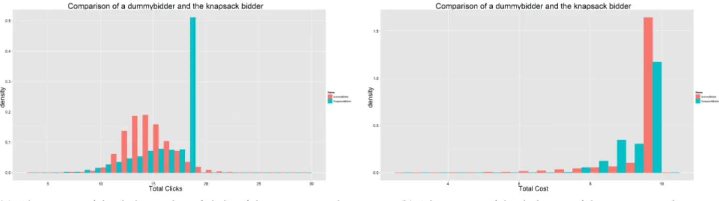
In table 7.1 some results of the simulation can be seen. In this scenario, the knapsack algorithm was compared to a bidder that always bids 0.2, the min-imum bid of the auction. If in this case the knapsack algorithm exhausts its budget before the end of the auction, it will lose to the dummy bidder, because this bidder is likely to still have budget left. In figure 7.2a histograms of con-versions are plotted, from which it is possible to conclude that the knapsack approach clearly is distributed with a higher average than that of the dummy approach. Furthermore, in figure 7.2b is a histogram of the cost of the two ap-proaches. From this it is clear that the knapsack approach is far better capable of spending its entire budget, thus optimising the number of clicks and con-versions. However, when looking again at table 7.1 it becomes clear that the cost per click and cost per conversion is almost exactly equal to the dummy approach. Assuming that a conversion has a positive return, the knapsack ap-proach is far better in this case.
24 Results Average Clicks Average Conversions Average Cost Average Cost/Click Average Cost/Conversion DummyBidder 11.32 1.14 2.26 0.20 1.98 KnapsackBidder 23.00 2.31 4.60 0.20 1.99
Table 7.1: Statistics from the simulation with a dummy bidder bidding 0.2, sce-nario 1
(a) A histogram of the daily number of conversions of the two ap-proaches
(b) A histogram of the daily cost of the two approaches
Figure 7.2: Histograms comparing the knapsack- and dummy-bidder in sce-nario 1
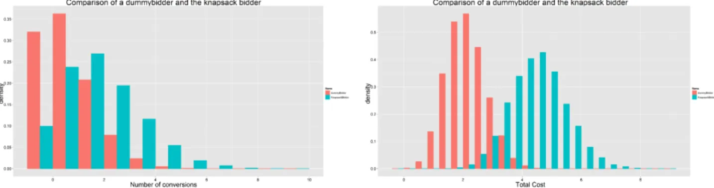
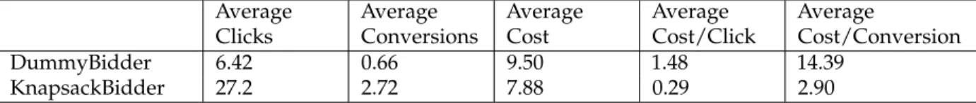
25 Results Average Clicks Average Conversions Average Cost Average Cost/Click Average Cost/Conversion DummyBidder 6.42 0.66 9.50 1.48 14.39 KnapsackBidder 27.2 2.72 7.88 0.29 2.90
Table 7.2: Statistics from the simulation with a dummy bidder bidding uniform between 0.2 and 10, scenario 2
Average Clicks Average Conversions Average Cost Average Cost/Click Average Cost/Conversion DummyBidder 12.1 1.21 8.64 0.714 7.14 KnapsackBidder 21.4 2.15 8.77 0.410 4.08
Table 7.3: Statistics from the simulation with a dummy bidder bidding uni-formly between 0.2 and 3, scenario 3
Bidding against a random bidder, scenario 2
Another case is a bidder that bids uniform randomly between the minimum-bid and the total budget over time. This represent a case that is totally different from the previous one. Here the total budget will probably have to be spent, while bidding in such a way so as to end in the top position as often as possible. A short overview of the results are in table 7.2. In the table it is easy to see that the algorithm is far better in this case as well. About the same cost is incurred, but almost double the amount of clicks - and thus conversions - is obtained. The histograms in this case are similar to the previous simulation and are therefore omitted.
Bidding against a random bidder, scenario 3
Perhaps it is not very realistic to bid over the entire range, as it is highly unlikely that someone would be willing to bid his entire daily budget just for one click. Therefore in this case, a dummy bidder was constructed that bids uniformly between 0.2, the minimum bid, and 3, about one third of the total budget. The results of this simulation are in table 7.3.
Bidding against a constant bidder, scenario 4
Another simulation was run with a dummy bidder that constantly bids the same value, 1.4. This is probably also a very realistic case as most advertisers will probably not constantly re-optimise their biddings. The results of this sim-ulation are in table 7.4. The histograms of this simsim-ulation for both the number
26 Results Average Clicks Average Conversions Average Cost Average Cost/Click Average Cost/Conversion DummyBidder 12.5 1.25 9.8 0.784 7.84 KnapsackBidder 20.7 2.08 8.95 0.432 4.30
Table 7.4: Statistics from the simulation with a dummy bidder bidding 1.4, sce-nario 4
(a) A histogram of the daily number of clicks of the two approaches (b) A histogram of the daily cost of the two approaches Figure 7.3: Histograms comparing the knapsack- and dummybidder in
sce-nario 4
of clicks and the daily cost are also very interesting and these are in figures 7.3a and 7.3b.
From both figures and the table it can be seen that the results are still a lot bet-ter than the dummy-bidder that uses no algorithm, but randomly bids some-thing or constantly bids the same. The algorithm is better able to spend its budget and also gets a lot more conversion, while at the same time paying less money per conversion. An overview of all results for conversions from all four simulations can be seen in figure 7.4.
Simulating against the same algorithm
The previous results are all very convincing that using a knapsack approach outperforms some basic bidding strategies. But what happens when all bidders use an optimised approach is not obvious. Therefore, simulations were run with two bidders that both use the knapsack approach. To still have some difference between the two bidders, all parameters were kept equal except the epsilon. One is bidding using an epsilon of 1.5 and the other using an epsilon of 2. An overview of the results can be seen in 7.5.
27 Results
Figure 7.4: Barcharts with the results of the two strategies of all simulations Average Clicks Average Conversions Average Cost Average Cost/Click Average Cost/Conversion KnapsackBiddera 13.8 1.36 9.75 0.709 7.16 KnapsackBidderb 16.6 1.67 9.71 0.586 5.82 aUsing an epsilon of 1.5 bUsing an epsilon of 2
Table 7.5: Statistics from the simulation with two knapsack-bidders
Plots are omitted, but are similar to the previously shown plots of the dummy bidder and the knapsack bidder. This leads to the question what the optimal value of epsilon is. But this can not easily be determined as the optimal value of epsilon depends on the expected value of a conversion of the keyword and other bidders’ strategies. As these strategies are not known, it is impossible to determine what value of epsilon is optimal in general.
7.1.2
Using the algorithm on real data
28 Results
7.1.3
Optimising the algorithm
In the previous results, the values forUandLwere used from the algorithm andεwas chosen at a certain value. But what optimal values for these param-eters are is not clear and determining this is not straightforward. Fortunately the simulation program that was used in the previous sections runs very fast and therefore this could be used to determine the optimal value for these pa-rameters. The speed of the simulation was used in a variant of a genetic algo-rithm that was written in which a population of 100 knapsack bidders all get the chance to compete against the best bidder of the previous generation. As a measure of how successful an individual is, first a comparison based on the number of conversions obtained was used. If this was equal, then on the size of the budget that was left-over. If this was also equal, then on the number of clicks obtained. For every generation the same random seed was used for the simulation, this means that every individual of a generation had the same potential number of clicks and conversions, as the queries arrived in the same way. However for a new generation, a new random seed was used, so that the individual would not learn the best values just for a single auction, but would optimise for the general type of the auction.
More precisely, the genetic algorithm first generated an initial population of 100 knapsack-optimisers, all with an upperbound andεas a random sample from a continuous uniform distribution. The upperbound was sampled from a distribution with bounds 0 and 50 and theεwith bounds 0 and 2. Then ev-ery individual had a day to compete against the bidder that was best in the previous generation. For the first generation this was set to another knapsack-bidder who had value 2 for every parameter. After all simulations were run, the population was sorted in the way described in the previous paragraph.
Now to create a new generation, the best two knapsack-bidders were used to recombine into two children using 2-point cross-over. After this, the rest of the new generation is filled by random mutations of the best 5% of the current generation. The new parameter values were determined by adding a random sample from a normal distribution with zero mean andσstandard deviation to the old value, where both the upperbound and theεhave their ownσ. This
σis decreased by a small amount every generation so that in the beginning the population can ’jump around’ the fitness landscape to explore, but in the end can focus on one region and find the best local optimum. Then this new generation is set as the current generation and the entire process starts over again.
It is hard to determine a stopping criterion for this algorithm and therefore it was stopped ’by hand’. Because every generation has a totally different day to compete on, the number of clicks, conversions and cost varies a lot from day
29 Results
(a) The upperbound as it evolves from generation to generation (b) The epsilon as it evolves from generation to generation Figure 7.5: The epsilon and upperbound from generation to generation
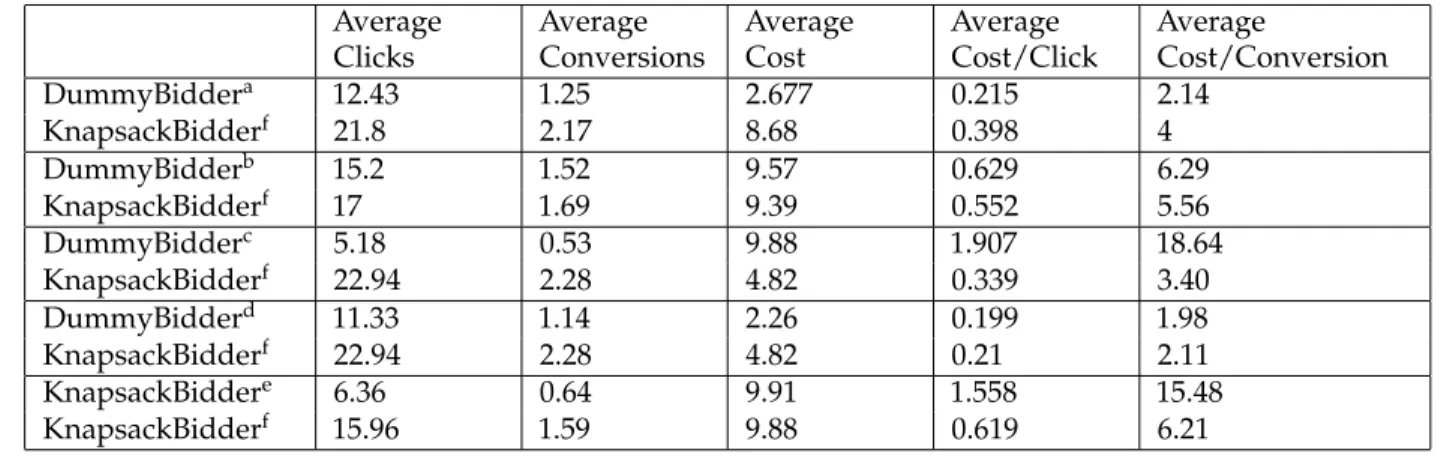
Average Clicks Average Conversions Average Cost Average Cost/Click Average Cost/Conversion DummyBiddera 12.43 1.25 2.677 0.215 2.14 KnapsackBidderf 21.8 2.17 8.68 0.398 4 DummyBidderb 15.2 1.52 9.57 0.629 6.29 KnapsackBidderf 17 1.69 9.39 0.552 5.56 DummyBidderc 5.18 0.53 9.88 1.907 18.64 KnapsackBidderf 22.94 2.28 4.82 0.339 3.40 DummyBidderd 11.33 1.14 2.26 0.199 1.98 KnapsackBidderf 22.94 2.28 4.82 0.21 2.11 KnapsackBiddere 6.36 0.64 9.91 1.558 15.48 KnapsackBidderf 15.96 1.59 9.88 0.619 6.21 aAlways bidding 0.4 bAlways bidding 1.4 cAlways bidding 4 dAlways bidding 0.21
eThe old knapsackbidder used in the simulations in section 7.1.1 f The optimised knapsack bidder
Table 7.6: Statistics from the simulation with the optimised knapsack-bidder
to day and no pattern can be seen in this. The upperbound andεdo converge to a certain value, as can be seen in figures 7.5a and 7.5b.
Now it is interesting to see what the algorithm does when again bidding against an opponent. Various simulations were run again, with the results of these summarized in table 7.6.
30 Results
What becomes most clear from these simulations is that the knapsack bidder has really learned to get better than a non-optimised knapsack bidder. Bidding against a bidder with constant bids has not really improved a lot.
7.1.4
Conclusion
It can immediately be seen that this method performs a lot better than bid-ding a constant amount. The algorithm always performs better and depenbid-ding on the amount the other bidder is bidding, it can perforum up to 4 times as good. And after optimising the bidder, it is also much better than another knapsack bidder that was not optimised.
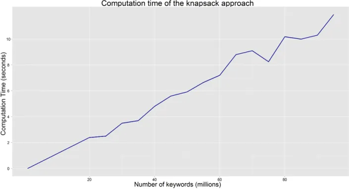
A big advantage of the method is that it adjusts its bids to the progress of the auction during the budget period, if more money is spent than initially expected, the bids get lower faster. But if on the other hand, the number of clicks is lower than expected, and thus less money is spent, the bids remain higher. This is a very desirable property, because a lot of other approaches make an estimate for the number of clicks during the day and then bid a fixed amount the entire budget period, hoping to spend it all during this period. If the actual situation during the day is other than expected, either the bid is too high and before the end of the budget period the budget is exhausted, or the bid is too low and budget is left over at the end of the budget period. It is not necessarily negative to have left-over budget, but under the assumption that the budget is there to get positive results, it would have been better to spend more. Another advantage is that this approach works on one keyword, so individual bids and return can be set per keyword, thus allowing for better fine-tuning of the model. Another very big upside to this approach is that it is very easy to compute a bid, as only one analytical formula needs to be computed. This is a very big advantage, as it is no problem to compute bids for tens of thousands of keywords instantly. See for instance figure 7.61, in which
the computation time of the method is plotted versus the number of keywords for which a bid is computed. The computation time grows linearly and is less than 12 seconds even for 95 million keywords.
A big downside to this approach is also that it works for one keyword. To fully utilise this approach, for every keyword (which can be as many as tens of thousands), every time a portion of the budget is spent, so every time someone clicks on one of the advertisements, all bids would have to be re-optimised. This could be circumvented by not always re-optimising but only on certain pre-defined moments in time or after a certain portion of the total budget is spent. Another downside is that the approach uses a per-keyword budget, whereas in reality a budget for all keywords in a campaign is set, and this is probably more desirable as well. Because spending more on one keyword is 1The inconsistent growth in the plot is due to both stochasticity in the keywords, since they were randomly generated, and because of other processes running on the computer
31 Results
Figure 7.6: The computation time for a growing number of keywords
not a problem if another keyword is less expensive than expected. Setting a budget over all keywords allows the costs to average out.
7.2
The Markov decision process approach
7.2.1
The MDP approach on generated data
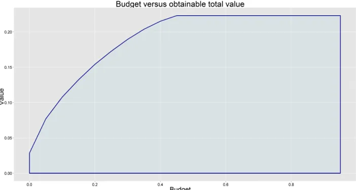
This approach computes advertising levels for all keywords simultaneously. In figure 7.7 a plot was made with 100 keywords, each having a number of impressions that is normally distributed with a mean of 1,000 and a standard deviation of 400; number of clicks that is normally distributed with a mean of 200 and a standard deviation of 50 and number of conversions that is normally distributed with a mean of 25 and a standard deviation of 10. For all keywords the cost per click was randomly sampled from a log-normal distribution with a mean of 1 and 0.7 standard deviation. The plot shows the expected optimal value that can be attained per user, versus the total budget that is allocated per user.
An interesting observation is that adding more and more budget helps less and less. This is logical, after a while more advertising will not help anymore.
32 Results
Figure 7.7: The expected optimal value (or return) per user versus the budget that is allocated per user
And that this increase is decreasing is also logical. If the algorithm chose the correct keywords, first the ones that yield the most should be chosen and after that the less performing keywords. That the line becomes a horizontal line is logical too, after the first position is obtained for every keyword, adding more budget does not help anything. The line also does not begin in the origin, because if no budget at all is spent, the user can still search for keywords and find KLM, only not through advertisements.
A big advantage of this approach is that it allows for direct computation of a lot of values of interest. Like in graph 7.7, it is possible to determine how much total value would be obtained by setting a certain budget. Or on the other hand, what would happen to that value if the cost per click would increase by 10%.
The downside of this approach is that a lot of values need to be known in advance. To generate the entire matrix that is needed to compute a strategy, all carry-over probabilities need to be known. And these are all values that are not measured currently and it is also very hard to do so. Furthermore, when optimising with for instance 10,000 keywords, for every advertising level a
33 Results
matrix is generated that has 10,000 x 10,000 size, so a matrix with 10,000,000 variables per advertising level. And if there are 4 advertising levels for all these keywords, for 40,000 variables the portion of time that is spent in that state need to be computed. In general, when optimiSing the number of variables becomes|X0|×|A|and the number of constraints is|X|+ 1. This imposes fairly heavy restrictions on the machine on which this computations are running, as this is quite a memory and time intensive operation.
Another downside is that the computations are all on a per-user basis, all results need to be translated back to the general situation in which you do not advertise for one specific user, but for anyone in the system. This is something that is not easily done, because beforehand it is not known how many users there will be on a given day. This gives the problem that since the budget is set per user, this would mean the budget itself becomes stochastic. Still the approach could provide valuable insights in for instance what the gain is per user that searches for ’KLM’ or what effect there would be when users have a 10% higher probability of converting even when not advertising.
7.2.2
Using the algorithm on real data
Confidential
7.3
Comparing the two methods
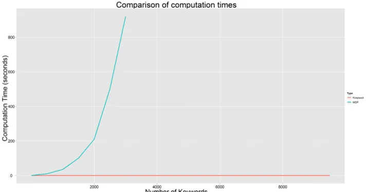
As already mentioned, both methods have their pros and cons. Which method is best is not easily said as both approaches can be used for other purposes. The knapsack approach allows for fast computation of bids per keyword and can optimise these bids during the budget period, on the other hand the MDP ap-proach can be used to optimise the budget itself, something that is not possible with the knapsack approach. Computing bids for actual keywords with the MDP approach is harder because of the high number of variables involved. Computing bids even for 10,000 keywords would take a very long time. In figure 7.8 a comparison is made of the two approaches in terms of computa-tion times. It can be seen that the Markov decision process approach takes a lot more time to compute and is also not as well scalable as the knapsack approach.
The problem with computation times can however be circumvented. But this comes at a cost. An approach to circumventing the long computation times would be to partition the keyword set into smaller sets and then optimising per set. This increases performance because an LP problem can be solved in time
O(n3.5)[21], wherenis the number of variables. If this set is partitioned in for
example 10 partitions, the computation time becomesO(10·(n
10)
34 Results
Figure 7.8: A comparison of the computation times of the two approaches
10·(n
10)
3.5<< n3.5, it is a lot faster to partition the keyword set. A graph with
this approach can be seen in figure 7.9.
The results are really good, with a performance increase of a factor of about 160. From the previous computation, one would perhaps expect an increase of about 316 - given the ratio 10·(10n)
3.5
n3.5 - butO(n
3.5)is worst case complexity.
Given the performance increase of a factor of about 160, it would appear the complexity in this case is aboutO(n3.2). This increase still does not make it
anywhere near as fast as the knapsack approach (the knapsack approach com-putes bids for about 40,000,000 keywords in 5 seconds, whereas the partitioned MDP approach computes bids for only 3,000 keywords), but it does allow for realistic computation times for a realistic keyword set.
So overall the knapsack approach can best be used to optimise bidding on keywords. Whereas at the same time the MDP approach can be used to per-form what-if analysis. If both approaches are combined in this way, both bid-ding and budgeting can be optimised to find the optimal values for both. Note however that these two things are linked heavily together and that higher bids require a higher budget and vice versa. This still makes optimising very
com-35 Results
Figure 7.9: The computation times of the partitioned approach
plicated, but no algorithm can be made to optimise both at the same time. This depends very much on the goals and preferences of an advertiser, so human input for this would still be needed.
7.4
Combining the two methods
Most interesting would be to combine the strong suits of both methods and at the same time leave out the disadvantages. The main difficulty in using the knapsack approach for all keywords is that it actually only works very well for one keyword, but is not able to capture relations between keywords and the total keyword-set. On the other hand, the MDP approach is very well able to capture these relations, but is not very well able to determine bids for one keyword. Fortunately, these two things do not overlap and therefore a ’hybrid’-approach can be used.
First, the MDP approach can be run with ample budget. This means that the algorithm is able to advertise with every keyword and is not limited in its spendings. When computations are complete, a probability distribution is found over all keywords which gives the probability of being in a certain state.
36 Results
Since there was ample budget, the algorithm is able to advertise on any key-word as much as it likes and therefore, the probability distribution that is ob-tained, actually gives the amount the algorithm would like to advertise on a certain keyword, relative to the other keywords. This value can then be used in the knapsack algorithm to allocate a per-keyword budget. Since every key-word in the knapsack approach needs a separate budget, exactly the portion that was determined in the MDP approach can be used as the portion of the total budget that is allocated to one keyword. Then computations can be made per keyword and bids are obtained. After spending a part of the budget, the budget needs to be re-allocated to the keywords, still according to the ratio that was obtained with the MDP approach.
Then, using just these values as the portion of the budget that the keyword is allowed to spend is not enough. These values only show what portion of the time there should be advertisements on keywordx, it does not take into account what the cost is of keeping this position. So to determine what portion of the budget a keyword is allowed to spend in the knapsack algorithm, the portion of time that was determined by the MDP is multiplied by the average cost per click of this keyword. Then all keywords get a part of the budget that is proportional to this value. When part of the budget is spent, this part is then divided over all keywords with the same proportion. This results in an algorithm that takes advantage of both the algorithms strengths, and uses these strengths to circumvent the algorithms weaknesses.
Chapter 8
Conclusion
This paper was started with the question: what strategy should be used to bid on advertisements at paid search channels? It is shown that utilising a com-bination of a knapsack-based approach and a Markov decision process model is a very good strategy that can improve performance up to 10% compared to bidding a fixed amount.
8.1
The adwords
First an analysis of the current situation was done. This showed that the cost of ranking first is generally justified, as the first position obtains a lot more clicks than any other position. Besides, it appeared that very often the bud-get is not entirely spent so there is still room for advertisements that are not displayed first to bid more.
8.2
The auction
It was found that the process of deciding how much and on which keywords to advertise can best be modeled as a knapsack problem. The main advantage is that it is possible to compute a bid for a single keyword. When comparing this model to the current situation - bidding a fixed amount -, an improvement in the number of clicks, while keeping the same budget, of about 10% can be obtained. Another big advantage of this approach is that it allows for fast com-putations which allows setting bids for thousands of keywords.
A downside is that the model requires some parameters and determining these can be tricky. Since the behaviour from day to day fluctuates a lot, as is shown in the analysis in chapter 3, it is difficult to determine whether today’s parameters are really better than yesterday’s, or that an observed change is the result of customer behaviour.
38 Conclusion
Utilising an MDP-based approach, as described in chapter 6, yields good re-sults for what-if analysis. It can be used to predict the possible result of changes in budget and how much advertising would be optimal for a single keyword within the total set of keywords. It is able to capture relations between key-words very well.
The downside of the described MDP-based approach is that it requires more parameters than are currently known, and these parameters are also hard to measure. Therefore assumptions are necessary and because of the difficulty of measuring these parameters, it is hard to determine exactly how well these assumptions are.
Combining both the MDP and the knapsack approach yields a good, total model that is both capable of dividing the total budget over all keywords and of setting bids per keyword. The problem that remains is the one of setting a total budget, but this is dependent on advertisement strategy and can not be solved solely by mathematics. The MDP model does give a prediction of what the result of setting a certain budget is.
8.3
Further work
The proposed knapsack model would need to compute a bid the moment an auction is held to yield the best results. In reality this is not possible because Google takes bids from its database and therefore fixed bids need to be set. A resolution to this can be re-optimising every so-many minutes with the latest results. Since the model proposed in 7.4 is already programmed to work with actual data as it is delivered by Google, implementing this algorithm to set bids for all keywords would not require a lot of work. What still needs to be set up is a connection between the current system that sets bids and evaluates the auctions and the optimiser so that the current situation can be downloaded, the model can be run and optimised