Explicit formulas for pricing of callable mortgage-backed securities in a case of prepayment rate negatively correlated with interest rates

(1)

Contents lists available atSciVerse ScienceDirect

Journal of Mathematical Analysis and

Applications

journal homepage:www.elsevier.com/locate/jmaa

Explicit formulas for pricing of callable mortgage-backed securities in a

case of prepayment rate negatively correlated with interest rates

✩

Xiao-song Qian

a,b,∗

, Li-shang Jiang

c,b

, Cheng-long Xu

c

, Sen Wu

c a_{Department of Mathematics, Soochow University, Suzhou 215006, PR China}

b_{Center for Financial Engineering, Soochow University, Suzhou 215006, PR China} c_{Department of Mathematics, Tongji University, Shanghai 200092, PR China}

a r t i c l e i n f o

Article history:

Received 24 February 2011 Available online 21 April 2012 Submitted by Vladimir Pozdnyakov Keywords:

Mortgage-backed securities Prepayment risk

Reduced form model Prepayment factor

a b s t r a c t

In this paper, we deal with the pricing of Mortgage-Backed Securities (MBS) in the reduced-form framework. Based on the ideas presented by Brunel and Jribi (2008) [8] and Rom-Poulsen (2007) [7], we introduce a stochastic processQt = e−

t

0λsds_{to model the}

prepayment factor and assume that the prepayment rateλtis inversely proportional to the

stochastic interest ratert, which follows a CIR process. Explicit formulas for pass-through

MBSs and semi-analytical solutions for Collateralized Mortgage Obligations (CMO) are obtained through PDE approaches. Based on the formulas, numerical results are provided to explain the dependence of MBS prices on mortgage parameters and the negative correlation between MBS prices and interest rates.

1. Introduction

In this paper, we present an intensity-based model to value callable mortgage backed securities. Mortgage-backed securities (MBS) are debt obligations that represent claims to the cash flows from pools of mortgage loans, most commonly on residential property. There are many types of MBSs. A pass-through mortgage-backed security is the simplest MBS, whose cash flows, both principal and interest, are passed through to the investor via an intermediary who retains a portion of the interest on cash flows as compensation for services rendered including guaranteeing these pass-through payments. A collateralized mortgage obligation (CMO), differs from a pass through in that the underlying mortgage pool is separated into different maturity tranches, and each tranche’s holder receives interest payments as long as the tranche’s principal amount has not been completely paid off. The senior tranche receives all initial principal payments until it is completely paid off, after which the next most senior tranche receives all the principle payments, and so on. Usually mortgagors have the options to fully or partially prepay their loans prior to the maturity dates. In this paper, the analysis of MBS mainly concentrates on the prepayments of principals prior to maturity.

To deal with the prepayment risk in MBS, different types of models have been developed. These models can be classified into two main categories known asstructuralmodels andreduced-formmodels. In structural models, the prepayment is a call option exercised by the mortgagor to minimize the cost of his mortgage. The prepayment decision is entirely determined within the model by option pricing approaches. In these models, differences in prepayment costs drive the heterogeneity among mortgagors making them prepay at different times. Although this endogenous approach can yield considerate

✩ _{This work is supported by National Basic Research Program of China (973 Program) 2007CB814903 and the PRC grant NSFC 10801115 and 11171256.} ∗_{Corresponding author at: Department of Mathematics, Soochow University, Suzhou 215006, PR China.}

E-mail addresses:qianxs@gmail.com,qian@yzu.edu.cn(X.-s. Qian),jianglsk@online.sh.cn(L.-s. Jiang),clxu601@online.sh.cn(C.-l. Xu), creamwusen@126.com(S. Wu).

(2)

insights into the workings of idealized mortgages, it is usually difficult to employ these models for the purpose of empirical estimation. Examples of this type of models are [1–3].

In reduced-form models, however, the prepayment is no longer internally determined but rather directly modeled as a function of some exogenous random processes. Because of its flexibility and lack of dependence on unobservable factors, this kind of model is easily estimated by fitting it to observed prepayment data, and the MBS prices are then found either by Monte Carlo simulations, finite difference or lattice methods (see, for example, [4,5]). Recently, reduced-form models have emerged that use techniques from credit risk modeling. Goncharov [6] developed a general intensity-based prepayment model with an endogenously defined mortgage rate process. Rom-Poulsen [7] obtained semi-analytical solutions for the value of fixed-rate callable MBSs by presuming the mortgage pool size taking an intensity-base model. Brunel and Jribi [8]modeled the prepayment risk by introducing a prepayment factor

(

Qt

)

t≥0which represents the percentage of the

initial loan still outstanding at timet. One advantage of Brunel’s model is that details of the debt pool are not needed for purposes of calibration. Brunel and Jribi [8] only considered the situation where short term risk-free interest rate and the prepayment rate are all constants. However, these dynamic rates do not behave constantly in practice. Usually prepayment rates would rise when interest rates fall because the mortgagors would have more incentive to refinance their mortgages, whereas prepayment rates would fall when interest rates rise because the mortgagors would like to preserve their mortgages in this case.

In the paper, based on the ideas presented in [8,7], we establish an intensity-based model on prepayment risk. The short term rate is modeled as a CIR process and the prepayment rate is in inverse proportion to the interest rate, that is, it follows an inverse CIR process, which was first proposed by Ahn and Gao [9] and intensively studied by Hurd and Kuznetsov [10]. Using this model, we study the pricing of pass-through securities and sequential pay CMOs.

We only consider default-free MBSs in this paper. In many regions and countries, MBSs are usually based on mortgages that are guaranteed by a government agency for payments of principals and interests. The MBSs created by these agencies have little or no credit risk. In particular, after the subprime crisis, financial institutions have significantly improved thresholds for residential mortgages. For example, in China, a mortgagor usually has to make a downpayment of at least 30%, and the probability of default would be quite small in these scenarios. Papers that include the default option are [11–13] etc. The rest of the paper is organized as follows. The next section is devoted to the construction of the dynamic prepayment model. In the third section, we derive the pricing equation for MBSs and give an explicit pricing formula using a change of variables technique. In the fourth section we consider the collateralized mortgage obligations with sequential pay tranche structures and a semi-analytical solution is obtained. Numerical results are worked in Section5. At last we conclude our paper.

2. Dynamic prepayment model

The most common method for amortizing an interest-bearing loan is an installment loan, that is, a loan which is repaid with a fixed number of equal-sized periodic payments. Each cash-flow pays the interest on the outstanding balance and part of the principal. Considering a pool of amortizing loans, we denote byK0

t the future outstanding principal balance at timet

scheduled at timet

=

0 andKtthe resulting outstanding principal balance at timet. Without loss of generality, we assume

that the outstanding balance at timet

=

0 is equal to 1. We denoteT as the loan maturity,r0as the constant mortgage

interest rate andxas the constant payment rate.1_Then_K0

t satisfies the following differential equation:







dK_t0 dt

=

r0K 0 t

−

x

,

K₀0

=

1

,

K_T0

=

0

.

(2.1)

Solving the equation, we obtain K_t0

=

e r0t

₋

_er0T 1

−

er0T

,

(2.2) x

=

r0e r0T er0T

−

1

.

(2.3)

We model the prepayment risk by introducing the prepayment factor process

(

Qt

)

t≥0as in [8], which represents the

fraction of the resulting outstanding principal balance over the scheduled outstanding principal balance at timet, that is, Qt

=

Kt

K_t0

,

0

≤

t

≤

T

.

(2.4)

1 Herexis an average rate of payment for the whole pool. When prepayments occur, it is possible that the actual instantaneous payment rate is less thanx.

(3)

By definition,Qtis a positive process with initial valueQ0

=

1. We denote

λ

tthe continuous exponential decreasing rate of

Qtand call it prepayment rate. Then the link between

λ

tandQtis as following:







dQt Qt

= −

λ

_tdt Q0

=

1

.

(2.5)

Solving the Eq.(2.5), we get the expression ofQt:

Qt

=

e−

t

0λsds

.

_(2.6)

As we discussed previously, the prepayment rate

λ

tshould be negatively correlated with short term default-free interest

ratert. Let us consider the simplest case as follows

λ

t

=

α

rt

+

β

_t

,

(2.7)

where

α

is a constant and

β

t is a stochastic process which describes the influence of all other factors to the mortgagor’s

prepayment decision besides the interest ratert. When pricing MBS by prepayment intensity, one important property must

be fulfilled, that is, the prepayment rate

λ

tshould always be positive.2For this reason, the short term default-free interest

ratertand the process

β

tare assumed to satisfy CIR processes as follows

drt

=

κ

1

(θ

1

−

rt

)

dt

+

σ

1

√

rtdWt1

,

(2.8) d

β

t

=

κ

2

(θ

2

−

β

t

)

dt

+

σ

2



β

tdWt2

,

(2.9)

where

κ

i

, θ

i

, σ

i

(

i

=

1

,

2

)

are positive constants satisfying

2

κ

i

θ

i

> σ

i2

, (

i

=

1

,

2

)

(2.10)

andWi

t

(

i

=

1

,

2

)

are standard Brownian motions independent of each other under the risk-neutral probability measureQ.3

It is well known that under the condition(2.10)the processesrtand

β

tare all positive (see [14]). Then we can derive from

(2.4),(2.6)and(2.7)that Kt

=

e −t 0 _α rs+βs  ds K_t0

,

(2.11) and dKt

=

e −t 0 _α rs+βs  ds



−



α

rt

+

β

_t



K_t0

+

(

K_t0

)

′



dt

.

(2.12)

3. MBS pricing model and explicit formulas

Mortgage-backed securities are also known as mortgage pass-through securities, because their income from the underlying pools of loans, formed from residential or commercial loans or from a mixture of both, are passed through to the bondholders. An investor who owns the MBS is entitled to receive collections of interest and principal, including prepayments. However, a small portion of the interest collections is not passed through. Instead, it is used to cover expenses of the deal, which is called the servicing fee and the guarantee fee. Thus, a MBS has a ‘‘pass-through rate’’y0, which is the

net rate at which investors receive the interest on the principal balance of the mortgage loans backing the security. In the time interval

(

t

,

t

+

dt

)

, the investor’s cash flow is

−

dKt

+

y0Ktdt

,

(3.1)

which is composed of two parts, that is, the principal redemption part

−dK

tand the interest rate cash flow party0Ktdt.

LetFtbe the investor’s information filtration at timet, then the price of the pass-through security at timetis

Pt

=

EQ



T t e− τ t rsds

(

₋

_dK τ

+

y0Kτd

τ)



Ft



,

(3.2)

2 The readers may wonder that the fact that the prepayment rateλtis always positive seems to violate the mortgagor’s optimal behavior when interest

rates are high. But we do not consider a single mortgagor’s behavior here. We study the prepayment behavior for a pool of amortizing loans. Even when interest rates are high, it may be possible that a small portion of mortgagors in the pool still want to prepay their mortgages for some particular reasons. Besides,λtcould tend to zero theoretically, which means there is almost no prepayment.

(4)

where the expectation is taken under the risk-neutral probability measureQ. Substituting(2.11)and(2.12)into(3.2), we get Pt

=

e −t 0 _α rs+βs  ds EQ



T t e− τ t  rs+_rsα+βs  ds



α

K_τ0 r_τ

+

β

τK 0 τ

+

y0K_τ0

−

(

K_τ0

)

′



d

τ



Ft



.

(3.3)

Using the Markov property of the process

(

rt

, β

t

)

(t≥0), we can replace the conditional expectation in the above equation with a functionHoft

,

rtand

β

t(see [15]), that is

Pt

=

e −t 0 _α rs+βs  ds



T t H

(

t

,

rt

, β

t

;

τ)

d

τ,

(3.4) where H

(

t

,

r

, β

;

τ)

=

_EQ



e− τ t  rs+α rs+βs  ds



α

K_τ0 r_τ

+

β

τK 0 τ

+

y0K_τ0

−

(

K_τ0

)

′





rt

=

r

, β

t

=

β



.

(3.5)

Using the Feynman–Kac formula, we can easily obtained from(2.8),(2.9)and(3.5)thatH

(

t

,

r

, β

;

τ)

satisfies the following partial differential equation











∂

H

∂

t

+

1 2

σ

2 1r

∂

2_H

∂

r2

+

1 2

σ

2 2

β

∂

2_H

∂β

2

+

κ

1

(θ

1

−

r

)

∂

H

∂

r

+

κ

2

(θ

2

−

β)

∂

H

∂β

−



r

+

α

r

+

β



H

=

0

,

(

0

<

r

<

∞

,

0

< β <

∞

,

0

≤

t

< τ),

H

(τ,

r

, β

;

τ)

=

g

(

r

, β, τ), (

0

<

r

<

∞

,

0

< β <

∞

),

(3.6) where g

(

r

, β, τ)

=

α

K 0 τ r

+

β

K 0 τ

+

y0Kτ0

−

(

Kτ0

)

′

.

(3.7)

We introduce the transformationH

(

t

,

r

, β

;

τ)

=

rb1_e−a1r−a2β−b2(τ−t)_U

(

_t

,

_r

, β

_;

τ)

_{, where}

ai

=

−

κ

_i

+



κ

2 i

+

2

σ

i2

σ

2 i

, (

i

=

1

,

2

),

b1

=

−

κ

₁

θ

₁

+

σ

₁2/2

+



(κ

1

θ

1

−

σ

12/2

)

2

+

2

σ

12

α

σ

2 1

,

(3.8) b2

=

κ

1

θ

1a1

+

κ

1b1

+

σ

12a1b1

+

κ

2

θ

2a2

.

Then an easy calculation will show that the functionU

(

t

,

r

, β

;

τ)











∂

U

∂

t

+

1 2

σ

2 1r

∂

2_U

∂

r2

+

1 2

σ

2 2

β

∂

2_U

∂β

2

+

κ

′ 1

(θ

′ 1

−

r

)

∂

U

∂

r

+

κ

′ 2

(θ

′ 2

−

β)

∂

U

∂β

=

0

,

(

0

<

r

<

∞

,

0

< β <

∞

,

0

≤

t

< τ),

U

(τ,

r

, β

;

τ)

=

r−b1_ea1r+a2β_g

(

_r

, β, τ), (

₀

<

_r

<

_∞

,

₀

< β <

_∞

),

(3.9) where

κ

′ i

=



κ

2 i

+

2

σ

i2

, (

i

=

1

,

2

),

θ

′ 1

=

κ

1

θ

1

+

b1

σ

12



κ

2 1

+

2

σ

2 1

,

θ

′ 2

=

κ

2

θ

2



κ

2 2

+

2

σ

2 2

.

(3.10)

To solve Eq.(3.9), we need the following lemma.

Lemma 3.1. The fundamental solution to the following equation







∂

U

∂

t

+

1 2

σ

2 1r

∂

2_U

∂

r2

+

1 2

σ

2 2

β

∂

2_U

∂β

2

+

κ

′ 1

(θ

′ 1

−

r

)

∂

U

∂

r

+

κ

′ 2

(θ

′ 2

−

β)

∂

U

∂β

=

0 U

(

r

, β, τ

;

y1

,

y2

, τ)

=

δ(

r

−

y1

)δ(β

−

y2

)

(3.11) is G1

(

r

,

t;y1

, τ)

·

G2

(β,

t

;

y2

, τ)

(3.12)

(5)

where

δ(

· )

is Dirac delta function and the function Gi

(

i

=

1

,

2

)

is defined by Gi

(

xi

,

t;yi

, τ)

=

cie−ui−vi



v

i ui

q

i/2 Iqi



2

(

ui

v

i

)

1/2



,

(3.13) and ci

=

2

κ

_i′

σ

2 i

(

1

−

e −κ′_i(τ−t)

₎

,

ui

=

ci

·

xi

·

e−κ ′ i(τ−t) _{with x} 1

=

r

,

x2

=

β,

v

i

=

ci

·

yi

,

qi

=

2

κ

′ i

θ

′ i

σ

2 i

−

1

,

Iqi

(

· )

is the modified Bessel function of the first kind of order qi,

Iqi



2

(

ui

v

i

)

1/2



=

(

ui

v

i

)

qi/2 ∞



k=0

(

ui

v

i

)

k k!Γ

(

qi

+

k

+

1

)

.

Proof. It is well known (see [16]) thatGi

(

i

=

1

,

2

)

as functions of

(

xi

,

t

)

with parameters

(

yi

, τ)

are fundamental solutions

to the following equations corresponding to CIR processes with parameters

κ

′

i

, θ

′ i and

σ

i

(

i

=

1

,

2

)

∂

u

∂

t

+

1 2

σ

2 i xi

∂

2_u

∂

x2_i

+

κ

′ i

(θ

′ i

−

xi

)

∂

u

∂

xi

=

0

.

Then we know from the theory of parabolic equations thatG1

·

G2as function of

(

t

,

r

, β)

with parameters

(τ,

y1

,

y2

)

is the

fundamental solution to Eq.(3.11).

Then we can deduce that the solution to Eq.(3.9)is U

(

t

,

r

, β

;

τ)

=



∞ 0



∞ 0 y−b1 1 e a1y1+a2y2_g

(

_y 1

,

y2

, τ)

G1

(

r

,

t;y1

, τ)

G2

(β,

t;y2

, τ)

dy1dy2

,

=



∞ 0



∞ 0 y−b1 1 e a1y1+a2y2



α

K0 τ y1

+

K_τ0y2

+

y0K_τ0

−

(

K_τ0

)

′



G1

·

G2dy1dy2

,

=

α

K_τ0



∞ ea1y1_y−b1−1 1 G1

(

r

,

t;y1

, τ)

dy1

 

∞ 0 ea2y2_G 2

(β,

t;y2

, τ)

dy2



+

K_τ0



∞ 0 ea1y1_y−b1 1 G1

(

r

,

t;y1

, τ)

dy1

 

∞ 0 ea2y2_y 2G2

(β,

t;y2

, τ)

dy2



+



y0K_τ0

−

(

K_τ0

)

′





∞ 0 ea1y1_y−b1 1 G1

(

r

,

t;y1

, τ)

dy1

 

∞ 0 ea2y2_G 2

(β,

t

;

y2

, τ)

dy2



.

(3.14) It is easy to verify that



∞ 0 ea1y1_y−b1 1 G1

(

r

,

t;y1

, τ)

dy1

=



∞ 0 ea1v1/c1



v

1 c1



−b1 c1e−u1−v1



v

1 u1

q

1/2 Iq1



2

√

u1

v

1



1 c1 d

v

1

=

cb1 1 e −u1_u−q1/2 1



∞ 0 e(a1/c1−1)v1

v

q1/2−b1 1 ∞



k=0 1 k!Γ

(

q1

+

k

+

1

)

(

u1

v

1

)

k+q1/2d

v

1

=

cb1 1 e −u1 ∞



k=0 uk 1 k!Γ

(

q1

+

k

+

1

)



∞ 0 e−(1−a1/c1)v1

v

q1+k−b1 1 d

v

1

=

c q1+1 1 e −u1

(

c1

−

a1

)

q1−b1+1 ∞



k=0 Γ

(

q1

+

k

−

b1

+

1

)

k!Γ

(

q1

+

k

+

1

)



c1u1 c1

−

a1

k

=

c q1+1 1 e −u1

(

c1

−

a1

)

q1−b1+1

·

Γ

(

q1

−

b1

+

1

)

Γ

(

q1

+

1

)

∞



k=0

(

q1

−

b1

+

1

)

k k!

(

q1

+

1

)

k



c1u1 c1

−

a1

k

=

c q1+1 1 e −u1

(

c1

−

a1

)

q1−b1+1

·

Γ

(

q1

−

b1

+

1

)

Γ

(

q1

+

1

)

·

M



q1

−

b1

+

1

,

q1

+

1

,

c1u1 c1

−

a1



,

(3.15)

(6)

and



∞ 0 ea2y2_G 2

(β,

t;y2

, τ)

dy2

=



∞ 0 ea2v2/c2_c 2e−u2−v2



v

2 u2

q

2/2 Iq2



2

√

u2

v

2



1 c2 d

v

2

=

e−u2_u−q2/2 2



∞ 0 e(a2/c2−1)v2

v

q2/2 2 ∞



k=0 1 k!Γ

(

q2

+

k

+

1

)

(

u2

v

2

)

k+q2/2d

v

2

=

e−u2 ∞



k=0 uk₂ k!Γ

(

q2

+

k

+

1

)



∞ 0 e−(1−a2/c2)v2

v

q2+k 2 d

v

2

=

c q2+1 2 e −u2

(

c2

−

a2

)

q2+1 ∞



k=0 1 k!



c2u2 c2

−

a2

k

=

c q2+1 2

(

c2

−

a2

)

q2+1 e a₂u₂ c₂−a₂

,

_(3.16) whereM

(µ, ν,

z

)

=



∞ k=0 (µ)k k!(ν)kz

k_{is the confluent hypergeometric function and}

_(µ)

kdenotes the shifted factorial defined

by

(µ)

k

=

µ(µ

+

1

)

· · ·

(µ

+

k

−

1

)

fork

>

0

,

(µ)

0

≡

1

.

A similar calculation leads to



∞ 0 ea1y1_y−b1−1 1 G

(

r

,

t;y1

, τ)

dy1

=

cq1+1 1 e −u1

(

c1

−

a1

)

q1−b1

·

Γ

(

q1

−

b1

)

Γ

(

q1

+

1

)

·

M



q1

−

b1

,

q1

+

1

,

c1u1 c1

−

a1



,

(3.17) and



∞ 0 ea2y2_y 2G2

(β,

t;y2

, τ)

dy2

=

cq2+1 2

(

c2

−

a2

)

q2+2 e a₂u₂ c2−a2



q2

+

1

+

c2u2 c2

−

a2



.

(3.18)

Substituting(3.15)–(3.18)into(3.14), we obtain the explicit expression for the functionU

(

t

,

r;

τ)

U

(

t

,

r

, β

;

τ)

=

α

K_τ0M1

(

t

,

r;

τ)

N1

(

t

, β

;

τ)

+

K_τ0M2

(

t

,

r;

τ)

N2

(

t

, β

;

τ)

+



y0K_τ0

−

(

K_τ0

)

′



M2

(

t

,

r;

τ)

N1

(

t

, β

;

τ),

(3.19) withK0 τ defined by(2.2)and M1

(

t

,

r;

τ)

=

cq1+1 1 e −u1

(

c1

−

a1

)

q1−b1

·

Γ

(

q1

−

b1

)

Γ

(

q1

+

1

)

·

M



q1

−

b1

,

q1

+

1

,

c1u1 c1

−

a1



,

M2

(

t

,

r;

τ)

=

cq1+1 1 e −u1

(

c1

−

a1

)

q1−b1+1

·

Γ

(

q1

−

b1

+

1

)

Γ

(

q1

+

1

)

·

M



q1

−

b1

+

1

,

q1

+

1

,

c1u1 c1

−

a1



,

N1

(

t

, β

;

τ)

=

cq2+1 2

(

c2

−

a2

)

q2+1 e a2u2 c₂−a₂

,

N2

(

t

, β

;

τ)

=

cq2+1 2

(

c₂

−

a₂

)

q2+2e a2u2 c2−a2

· 

q2

+

1

+

c2u2 c₂

−

a₂



.

Then we can conclude this section by the following theorem

Theorem 3.2. The price of pass-through MBS Ptcan be expressed as

Pt

=

e −t 0  α rs+βs  ds



T t H

(

t

,

rt

, β

t

;

τ)

d

τ,

(3.20) where H

(

t

,

r

, β

;

τ)

=

rb1_e−a1r−a2β−b2(τ−t)_U

(

_t

,

_r

, β

_;

τ)

with ai

,

bi

(

i

=

1

,

2

)

defined by(3.8)and U

(

t

,

r;

τ)

defined by(3.19).

4. Sequential pay CMO

In this section, we study the structured exposure on the mortgages and the resulting amortization schedule is more complex. To simplify the derivation, we assume that the prepayment rate

λ

thas the following form

λ

t

=

α

rt

(7)

where

α

and

β

are all positive constants, and the interest rate satisfies drt

=

κ(θ

−

rt

)

dt

+

σ

√

rtdWt (4.2)

where

κ, θ, σ

are positive constants satisfying 2

κθ > σ

2 _and_W

t is a stand Brownian Motion under the risk-neutral

probability measureQ. The case that

β

follows a CIR process can be discussed similarly. We introduce a path-dependent variableJt: Jt

=



t 0

α

rs ds

.

(4.3)

Then the resulting outstanding principal balanceKtcan be expressed as

Kt

=

e− t 0λsds_K0 t

=

e −Jt−βt_K0 t

,

(4.4) and dKt

=

e−Jt−βt



−



α

rt

+

β



K_t0

+

(

K_t0

)

′



dt

,

(4.5) withK_t0defined by(2.2).

One of the demands that drove the design of CMOs was for mortgaged-backed securities with a wider range of maturities. The sequential pay CMO structures redirect principal payments sequentially to individual tranches. Principal payments go to senior tranche with the shortest stated maturity until it is completely redeemed, then allocated to the next class. Continue in this manner until all the securities in the structure are retired. For a mezzanine tranche with attachment pointAand detachment pointB, we define its outstanding balance at timetas

KAB

=











1

,

Kt

≥

B

,

Kt

−

A B

−

A

,

A

<

Kt

<

B

,

0

,

Kt

≤

A

.

(4.6)

In the time interval

(

t

,

t

+

dt

)

, the cash flow of

(

A

,

B

)

tranche is

−

dK_tAB

+

y0KtABdt

.

(4.7)

Then the

(

A

,

B

)

tranche security price at timetwill be P_tAB

=

_EQ

 

₍

_−dK

AB t

+

y0KtABd

τ)



Ft



,

(4.8)

where the expectation is taken under the risk-neutral probability measureQandFtis the investor’s information filtration

at timet. From(4.6),K_tABcan also be expressed as K_tAB

=

Kt

−

A

B

−

A1{A<Kt≤B}

+

1{Kt>B}

,

(4.9)

where1_Ωis the character function of the setΩ. Therefore dK_tAB

=

dKt

B

−

A1{A<Kt≤B}

.

(4.10)

Substituting(4.4),(4.5),(4.9)and(4.10)into(4.8), we have P_tAB

=

_EQ





−

dKτ B

−

A1{A<Kτ≤B}

+

y0 K_τ

−

A B

−

A1{A<Kτ≤B}d

τ

+

y01{Kτ>B}d

τ





Ft



=

_EQ











e−Jτ−βτ



α rτ

+

β

+

y0



K_τ0

−

(

K_τ0

)

′



−

y0A B

−

A 1{A<e−Jτ−βτKτ0≤B}

+

y01{e−J_τ−βτ_K0 τ>B}





d

τ



Ft





=



T 0 HAB

(

t

,

rt

,

Jt

;

τ)

d

τ,

(4.11)

(8)

where we have used the Markov property of processes

(

rt

,

Jt

)

(t≥0)in the last equality and HAB

(

t

,

r

,

J;

τ)

=

_EQ





e −τ t rsds





e−Jτ−βτ



α rτ

+

β

+

y0



K0 τ

−

(

Kτ0

)

′



−

y0A B

−

A 1{A<e−Jτ−βτKτ0≤B}

+

y01{e−J_τ−βτK_τ0>B}







rt

=

r

,

Jt

=

J





.

(4.12)

From(4.1),(4.2)and(4.12), using Feynman–Kac formula, we can easily obtain thatHAB

₍

_t

_,

_r

_,

_J;

_τ)

_{satisfies the following}

PDE problem











∂

HAB

∂

t

+

α

r

∂

HAB

∂

J

+

1 2

σ

2_r

∂

2_HAB

∂

r2

+

κ(θ

−

r

)

∂

HAB

∂

r

−

rH AB

₌

₀

_,

(

0

<

r

<

∞

,

0

≤

J

<

∞

,

0

≤

t

< τ),

HAB

(τ,

r

,

J;

τ)

=

f

(

r

,

J

, τ), (

0

<

r

<

∞

,

0

≤

J

<

∞

),

(4.13) where f

(

r

,

J

, τ)

=

e −J−βτ



α r

+

β

+

y0



K_τ0

−

(

K_τ0

)

′



−

y0A B

−

A 1{A<e−J−βτKτ0≤B}

+

y01{e−J−βτKτ0>B}. We introduce the transformationHAB

(

t

,

r

,

J;

τ)

=

e−ar−b(τ−t)V

(

t

,

r

,

J;

τ),

where

a

=

−

κ

+

√

κ

2

₊

₂

_σ

2

σ

2

,

b

=

κθ

a

.

(4.14)

Then it is easy to verify thatV

(

t

,

r

,

J;

τ)







∂

V

∂

t

+

α

r

∂

V

∂

J

+

1 2

σ

2_r

∂

2V

∂

r2

+

κ

′

_(θ

′

₋

r

)

∂

V

∂

r

=

0

, (

0

<

r

<

∞

,

0

≤

J

<

∞

,

0

≤

t

< τ)

V

(τ,

r

,

J;

τ)

=

earf

(

r

,

J

, τ),

(

0

<

r

<

∞

,

0

≤

J

<

∞

),

(4.15) where

κ

′

₌



κ

2

₊

₂

σ

2

,

θ

′

₌

_√

κθ

κ

2

₊

₂

σ

2

.

(4.16)

Divide

[0

, τ

]

intoNtime steps:

0

=

t0

<

t1

<

· · ·

<

tN

=

τ,

(4.17)

wheretn

=

n∆tand∆t

=

_Nτ. Then we will use splitting method to give a semi-analytical solution to the convection diffusion

Eq.(4.15)bynsteps.

First we solve the following two equations in the area

{0

<

r

<

∞

,

0

≤

J

<

∞

,

tN−1

≤

t

<

tN

}:







∂

V′ N−1

∂

t

+

α

r

∂

V′ N−1

∂

J

=

0

,

(

0

≤

J

<

∞

,

tN−1

≤

t

<

tN

),

V_N′₋₁

(

tN

,

r

,

J

)

=

earf

(

r

,

J

, τ), (

0

≤

J

<

∞

)

(4.18) and







∂

VN−1

∂

t

+

1 2

σ

2_r

∂

2VN−1

∂

r2

+

κ

′

_(θ

′

₋

r

)

∂

VN−1

∂

r

=

0

, (

0

<

r

<

∞

,

tN−1

≤

t

<

tN

)

VN−1

(

tN

,

r

,

J

)

=

VN′−1

(

tN−1

,

r

,

J

),

(

0

<

r

<

∞

).

(4.19)

For fixed variabler, we can easily solve Eq.(4.18)to get V_N′₋₁

(

tN−1

,

r

,

J

)

=

earf



r

,

J

−

α

tN−1 r

, τ



.

(4.20)

Substituting(4.20)into(4.19)we can obtain the solution of Eq.(4.19)for fixed variableJ: VN−1

(

t

,

r

,

J

)

=



∞ 0 V_N′₋₁

(

tN−1

,

y

,

J

)

G

(

y

,

tN

;

r

,

t

)

dy

=



∞ 0 eayf



y

,

J

−

α

tN−1 y

, τ



G

(

y

,

tN

;

r

,

t

)

dy fortN−1

≤

t

<

tN

,

(4.21)

(9)

Fig. 1. Pass-through MBS prices as a function ofrandβ.

whereG

(

y

,

s;r

,

t

)

is the fundamental solution corresponding to CIR process with parameters

κ

′

, θ

′and

σ

: G

(

y

,

s;r

,

t

)

=

ce−u−v



u

v

q

/2 Iq



2

(

u

v)

1/2



,

(4.22) and c

=

2

κ

′

σ

2

(

₁

₋

_e−κ′₍_s₋_t₎

)

,

u

=

c

·

r

·

e−κ′(s−t)

,

v

=

c

·

y

,

q

=

2

κ

′

_θ

′

σ

2

−

1

.

Then we proceed by induction. IfVn+1has been obtained between time interval

[t

n+1

,

tn+2

)

for 0

≤

n

≤

N

−

2, We

continue to solve the following equations in the area

{0

<

r

<

∞

,

0

≤

J

<

∞

,

tn

≤

t

<

tn+1

}:







∂

V_n′

∂

t

+

α

r

∂

V_n′

∂

J

=

0

,

(

0

≤

J

<

∞

,

tn

≤

t

<

tn+1

),

V_n′

(

tn+1

,

r

,

J

)

=

Vn+1

(

tn+1

,

r

,

J

), (

0

≤

J

<

∞

)

(4.23) and







∂

Vn

∂

t

+

1 2

σ

2_r

∂

2_V n

∂

r2

+

κ

′

_(θ

′

₋

r

)

∂

Vn

∂

r

=

0

, (

0

<

r

<

∞

,

tn

≤

t

<

tn+1

)

Vn

(

tn+1

,

r

,

J

)

=

Vn′

(

tn

,

r

,

J

),

(

0

<

r

<

∞

).

(4.24)

Similar to the case ofn

=

N

−

1, we can get V_n′

(

tn

,

r

,

J

)

=

Vn+1



tn+1

,

r

,

J

−

α

tn r



,

(4.25) and Vn

(

t

,

r

,

J

)

=



∞ 0 Vn+1



tn+1

,

y

,

J

−

α

tn y



G

(

y

,

tn+1

;

r

,

t

)

dy

,

fortn

≤

t

<

tn+1

.

(4.26)

By induction, in each time interval

[

tn

,

tn+1

) (

n

=

0

,

1

, . . . ,

N

−

1

)

, we can get an approximate solutionVn

(

t

,

r

,

J

)

to

Eq.(4.15). Define

V_∆t

(

t

,

r

,

J

)

=

Vn

(

t

,

r

,

J

)

in

[

tn

,

tn−1

),

forn

=

0

,

1

, . . . ,

N

−

1

.

(4.27)

(10)

Fig. 2. MBS prices with different prepayment rate parameter values ofα.

Fig. 3. MBS prices with different volatility levels of interest rate. These derivation can be concluded as the following theorem:

Theorem 4.1. By introducing the path-dependent variable Jt

=



t

0

α

rsds, the

(

A

,

B

)

tranche security price P

AB

₍

_t

_,

_r

_,

_J

₎

_{can be} expressed by PAB

(

t

,

r

,

J

)

=



T t HAB

(

r

,

r

,

J;

τ)

d

τ,

(4.28)

where HAB

₍

_t

_,

_r

_,

_J;

_τ)

₌

_e−ar−b(τ−t)_V

₍

_t

_,

_r

_,

_J;

_τ)

_{with a}

_,

_{b defined by}_(4.14)_and

V

(

t

,

r

,

J;

τ)

=

lim

∆t→0V∆t

(

t

,

r

,

J;

τ).

(4.29)

5. Numerical results

In this section, numerical examples are presented to show how to price pass-through MBS by the explicit formula(3.20) obtained in Section3.

(11)

Fig. 4. MBS prices with different mean levels of interest rate.

Fig. 5. MBS prices with different mean reverting speeds of interest rate.

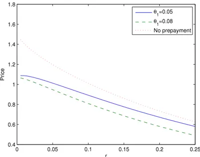
We first compute prices of pass-through MBS with the parameters

θ

1

=

0

.

05

, θ

2

=

0

.

04

, κ

1

=

0

.

3

, κ

2

=

0

.

2

, σ

1

=

0

.

12

, σ

2

=

0

.

1

,

r0

=

0

.

1

,

y0

=

0

.

08

, α

=

0

.

004

,

T

=

10. Then we take

β

= {0

.

04

,

0

.

08}. We see fromFig. 1that MBS

prices decrease with

β

value, which is obvious because larger

β

value means more chances for mortgagees to prepay and more risk for MBS. With the same parameters, we also plot the price curve when there is no prepayment. We see that the MBS prices with no prepayment risk are higher than the prices with prepayment risk, which holds for all the plots below.

InFigs. 2–8, we investigate the dependence of MBS prices on parameters of the prepayment model with

β

=

0

.

04. Fig. 2shows the influence of prepayment rate parameter

α

on MBS prices, with

α

= {

0

.

004

,

0

.

008

}

and other parameters equal to parameters inFig. 1. We know that the larger is the parameter

α

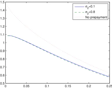
, the faster is the prepayment speed, and the cheaper are the MBSs prices, just as shown inFig. 2.

InFig. 3, we study the sensitivity of MBS prices to the volatility of interest rate, with

σ

1

= {0

.

12

,

0

.

10}and other

parameters equal to parameters inFig. 1. Usually when the interest rate volatility increases, the mortgagees will face more risk from changes of interest rates, and MBS prices should increase therefore. It is shown inFig. 3that the MBS prices increase with the volatility.

(12)

Fig. 6. MBS prices with different volatility levels of processβt.

Fig. 7. MBS prices with different mean levels of processβt.

Fig. 4shows the sensitivity of MBS prices to the mean value of interest rate, with

θ

1

= {0

.

05

,

0

.

08}and other parameters

equal to parameters inFig. 1. Usually the interest rate tends to achieve a higher level if it has a higher mean value, which will reduce the value of MBS. We can see the MBS price decreases with the mean value fromFig. 4.

Fig. 5shows the sensitivity of MBS prices to the mean reverting speed of interest rate, with

κ

1

= {0

.

3

,

0

.

4}and other

parameters equal to parameters inFig. 1. We can see that the faster is the mean reverting speed, the more stable is the MBS price. The reason is that the interest rate is more likely to maintain around its mean value if it has a higher speed of adjustment, which would cause less change of MBS prices.

We also investigate the influence of process

β

t’s parameters on MBS prices and get similar results as the interest rate’s

case. We see from theFigs. 6–8that MBS prices are not as sensitive to parameter adjustment of process

β

t as the interest

rate’s case. Indeed, the main prepayment factor is the interest rate in our model. So the process

β

_tdoes have less influence on MBS prices comparing with the interest rate.

6. Conclusion

In the reduced-form framework, we obtain explicit pricing formulas for pass-through MBS and semi-analytical solutions for sequential pay CMO under the assumptions that the prepayment rate and interest rate are inversely proportional to each

(13)

Fig. 8. MBS prices with different mean reverting speeds of processβt.

other and the interest rate movement is governed by a CIR process. These formulas will be very useful not only for valuation of MBS but also for estimating the prepayment risk from market information by using calibration technique without Monte Carlo simulation.

Acknowledgment

The authors are very grateful to the referee for his (or her) careful reading of the manuscript and several valuable comments.

References

[1] R. Stanton, Rational prepayment and the valuation of mortgage-backed securities, Rev. Financ. Stud. 8 (1995) 677–708. [2] J.B. Kau, D.C. Keenan, An overview of the option-theorectic pricing of mortgages, J. Hous. Res. 6 (1995) 217–244.

[3] L. Jiang, B. Bian, F. Yi, A parabolic variational inequality arising from the valuation fixed rate mortgage, European J. Appl. Math. 16 (2005) 361–383. [4] J.J. McConnell, M. Singh, Valuation and analysis of collateralized mortgage obligations, Manag. Sci. 39 (1993) 692–7090.

[5] E. Schwartz, W. Torous, Prepayment and the valuation of mortgage-backed securities, J. Finance 44 (1989) 375–392.

[6] Y. Goncharov, An intensity-based approach to the valuation of mortgage contracts and computation of the endogenous mortgage rate, Int. J. Theor. Appl. Finance 9 (2006) 889–914.

[7] N. Rom-Poulsen, Semi-analytical MBS Pricing, J. Real Estate Finance Econom. 34 (2007) 463–498. [8] V. Brunel, F. Jribi, Model-independant ABS duration approximation formulas, working paper, 2008.

[9] D.H. Ahn, B. Gao, A parametric nonlinear model of term structure dynamics, Rev. Financ. Stud. 12 (1999) 721–762.

[10] T.R. Hurd, A. Kuznetsov, Explicit formulas for Laplace transforms of stochastic integrals, Markov Process. Related Fields 14 (2008) 277–290. [11] E. Schwartz, W. Torous, Prepayment, default, and the valuation of mortgage pass-through securities, J. Business 65 (1992) 221–239.

[12] Y. Deng, J.M. Quigley, R.V. Order, Mortgage terminations, heterogeneity and the exercise of mortgage options, Econometrica 68 (2000) 275–307. [13] J.B. Kau, D.C. Keenan, A.A. Smurov, Reduced form mortgage pricing as an alternative to option-pricing models, J. Real Estate Finance and Econ. 33

(2006) 183–196.

[14] J.C. Cox, J.E. Ingersoll, S.A. Ross, A theory of the term structure of interest rates, Econometrica 53 (1985) 385–407. [15] S. Shreve, Stochastic Calculus for Finance II: Continuous-Time Models, in: Springer Finance, Springer, 2004. [16] W. Feller, Two singular diffusion problems, Ann. of Math. 54 (1951) 173–182.

[17] G.I. Marchuk, splitting and alternating direction methods, in: Ph.G. Ciarlet, J.-L. Lions (Eds.), Handbook of Numerical Analysis, Vol. I, North-Holland, Amsterdam, 1990.