Deep Visual Feature Learning for Vehicle Detection, Recognition and Re-identification

(1)

Deep Visual Feature Learning for

Vehicle Detection, Recognition and

Re-identification

Yi Zhou

School of Computing Sciences

University of East Anglia

This dissertation is submitted for the degree of

Doctor of Philosophy

(2)

(3)

Declaration

I hereby declare that this dissertation is all my own work. Parts of the thesis have been published in academic conference proceedings and journal articles. All these papers were authored / co-authored by me, Yi Zhou, during and as a result of my Ph.D. research.

Zhou, Y.and Shao, L., 2018, Jun. Viewpoint-aware Attentive Multi-view Inference for

Vehicle Re-identification. IEEE Conference on Computer Vision and Pattern Recognition

(CVPR), Salt Lake City, USA. IEEE. (Chapter 5)

Zhou, Y., Liu, L. and Shao, L., 2018. Vehicle Re-identification by Deep Hidden

Multi-View Inference. IEEE Transactions on Image Processing. DOI: 10.1109/TIP.2018.2819820

(Chapter 4)

Zhou, Y.and Shao, L., 2018, Mar. Vehicle Re-identification by Adversarial Bi-directional

LSTM Network. IEEE Winter Conference on Applications of Computer Vision (WACV),

Lake Tahoe, USA. IEEE. (Chapter 5)

Zhou, Y., Liu, L., Shao, L. and Mellor, M., 2017. Fast Automatic Vehicle Annotation for

Urban Traffic Surveillance. IEEE Transactions on Intelligent Transportation Systems. DOI:

10.1109/TITS.2017.2740303 (Chapter 3)

Zhou, Y.and Shao, L., 2017, Sep. Cross-View GAN Based Vehicle Generation for

Re-identification. Proceedings of theBritish Machine Vision Conference (BMVC), London,

UK. BMVA Press. [Oral. Acceptance rate 5.6%] (Chapter 4)

Zhou, Y., Liu, L., Shao, L. and Mellor, M., 2016, October. DAVE: a unified framework

for fast vehicle detection and annotation. In European Conference on Computer Vision

(ECCV)(pp. 278-293), Amsterdam. Springer International Publishing. (Chapter 3)

Liu, L.,Zhou, Y.and Shao, L., 2018. Deep Action Parsing in Videos with Large-scale

Synthesized Data. IEEE Transactions on Image Processing. DOI: 10.1109/TIP.2018.2813530

Liu, L.,Zhou, Y.and Shao, L., 2017, May. DAP3D-Net: Where, what and how actions

occur in videos?. InRobotics and Automation (ICRA), 2017 IEEE International Conference

on(pp. 138-145), Singapore. IEEE.

Yi Zhou April 2018

(4)

(5)

Acknowledgements

I would like to convey my gratefulness to the following, for their excellent help in my Ph.D. First of all, I would like to express my deepest thanks to my parents. They have been always providing their best love and unconditional support to me.

I would like to especially thank my primary supervisor Prof. Ling Shao, who has been kindly advising me in my Ph.D. and taught me two modules in my MSc. Under his supervision, he provides me with continuous support, patience, motivation, enthusiasm and immense knowledge which help me successfully finished my Ph.D. work. In addition to guiding me novel research ideas, he is also willing to discuss with me. He brought me into the interesting computer vision and machine learning research community.

I would like to thank the CREATEC Limited Corporation for the financial support of my living cost. Particularly, I very much appreciate Dr. Matt Mellor, who is the director of CREATEC, for his invaluable suggestions in doing industrial projects. I would also like to thank Dr. David Clark and Patrick Gordon for their technical support in collaborative projects.

I am indebted to Prof. Gerard Parr and Prof. Andy Day for their kind help in the later period of my Ph.D., and the great suggestions to my thesis.

I would like to thank my fellow colleagues in our laboratory. I am very grateful to my co-author, Dr. Li Liu, for his talented ideas and help, and other lab mates: Dr. Mengyang Yu, Dr. Feng Zheng, Dr. Yang Long, Dr. Ziyun Cai, Dr. Jungong Han, Dr. Lining Zhang, Yuming Shen, Bingzhang Hu, and Shidong Wang for their witty insights and refreshing discussions. My thanks also go to many visiting staffs and students in our lab: Dr. Haofeng Zhang, Dr. Xiaoming Liu, Yang Liu and Jin Li for their kind assistance. Thank all of them making daily research a very fun job.

The PGR director Dr. Katharina Huber and other administrative staffs in the School of Computing Sciences of the University of East Anglia, including Matthew Ladd and Binoop Pulikkottil John, have provided me with support in various matters. I appreciate their effort and kindness to me.

I would like to thank Dr. Jinchang Ren and Dr. Michal Mackiewicz as my examiners for carefully reviewing my thesis.

(6)

Finally, I would like to thank my loving wife Jiajun for her consistent encouragement to me when I was depressed and taking care of my life in the UK. To her, I dedicate this thesis.

(7)

Abstract

Along with the ever-increasing number of motor vehicles in current transportation systems, intelligent video surveillance and management becomes more necessary which is one of the important artificial intelligence fields. Vehicle-related problems are being widely explored and applied practically. Among various techniques, computer vision and machine learning algorithms have been the most popular ones since a vast of video/image surveillance data are available for research, nowadays. In this thesis, vision-based approaches for vehicle detection, recognition, and re-identification are extensively investigated. Moreover, to address different challenges, several novel methods are proposed to overcome weaknesses of previous works and achieve compelling performance.

Deep visual feature learning has been widely researched in the past five years and obtained huge progress in many applications including image classification, image retrieval, object detection, image segmentation and image generation. Compared with traditional machine learning methods which consist of hand-crafted feature extraction and shallow model learning, deep neural networks can learn hierarchical feature representations from low-level to high-level features to get more robust recognition precision. For some specific tasks, researchers prefer to embed feature learning and classification/regression methods into end-to-end models, which can benefit both the accuracy and efficiency. In this thesis, deep models are mainly investigated to study the research problems.

Vehicle detection is the most fundamental task in intelligent video surveillance but faces many challenges such as severe illumination and viewpoint variations, occlusions and multi-scale problems. Moreover, learning vehicles’ diverse attributes is also an interesting and valuable problem. To address these tasks and their difficulties, a fast framework of Detection and Annotation for Vehicles (DAVE) is presented, which effectively combines vehicle detection and attributes annotation. DAVE consists of two convolutional neural networks (CNNs): a fast vehicle proposal network (FVPN) for vehicle-like objects extraction and an attributes learning network (ALN) aiming to verify each proposal and infer each vehicle’s pose, color and type simultaneously. These two nets are jointly optimized so that the abundant latent knowledge learned from the ALN can be exploited to guide FVPN

(8)

training. Once the model is trained, it can achieve efficient vehicle detection and annotation for real-world traffic surveillance data.

The second research problem of the thesis focuses on vehicle re-identification (re-ID). Vehicle re-ID aims to identify a target vehicle in different cameras with non-overlapping views. It has received far less attention in the computer vision community than the prevalent person re-ID problem. Possible reasons for this slow progress are the lack of appropriate research data and the special 3D structure of a vehicle. Previous works have generally focused on some specific views (e.g. front), but these methods are less effective in realistic scenarios where vehicles usually appear in arbitrary viewpoints to cameras. In this thesis, I focus on the uncertainty of vehicle viewpoint in re-ID, proposing four different approaches to address the multi-view vehicle re-ID problem: (1) The Spatially Concatenated ConvNet (SCCN) in an encoder-decoder architecture is proposed to learn transformations across different viewpoints of a vehicle, and then spatially concatenate all the feature maps for further fusing them into a multi-view feature representation. (2) A Cross-View Generative Adversarial Network (XVGAN) is designed to take an input image’s feature as conditional embedding to effectively infer cross-view images. The features of the inferred and original images are combined to learn distance metrics for re-ID. (3) The great advantages of a bi-directional Long Short-Term Memory (LSTM) loop are investigated of modeling transformations across continuous view variation of a vehicle. (4) A Viewpoint-aware Attentive Multi-view Inference (VAMI) model is proposed, adopting a viewpoint-aware attention model to select core regions at different viewpoints and then performing multi-view feature inference by an adversarial training architecture.

(9)

List of figures

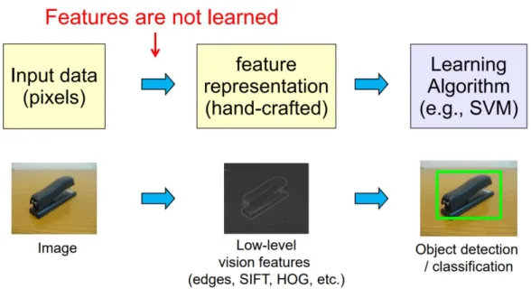
1.1 A traditional framework for addressing pattern recognition tasks, which

mainly consists of hand-crafted feature extraction and learning classifiers. . 2

1.2 A simple deep ConvNet for image classification. . . 3

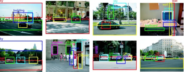
1.3 Illustration of the object detection task: localization + classification. . . 4

1.4 Some examples from the VIPeR [46] dataset for exploring person re-ID. Each pair of images are two shots of one person identity captured from different cameras. . . 6

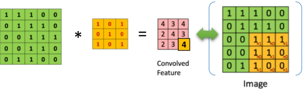
2.1 The convolution operation. The filters are convolved over a feature map in a sliding window fashion. . . 10

2.2 The max pooling operation. . . 11

2.3 An unrolled recurrent neural network architecture. . . 14

2.4 The architecture of Long Short-Term Memory. . . 16

2.5 The architecture of Gated Recurrent Unit. . . 16

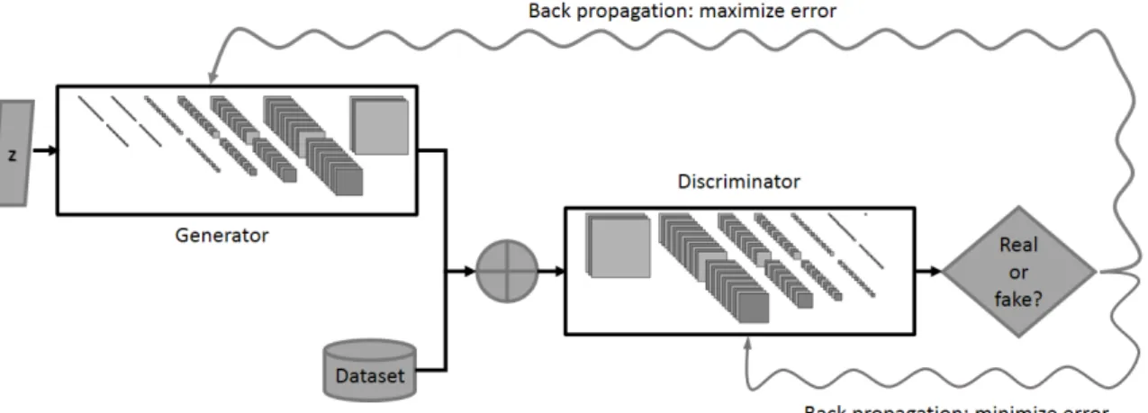
2.6 GAN mainly consists of a Generator and a Discriminator. The Generator network takes a random input and tries to generate a sample of data. The task of Discriminator network is to take input either from the real data or from the generator and try to predict whether the input is real or generated. . 26

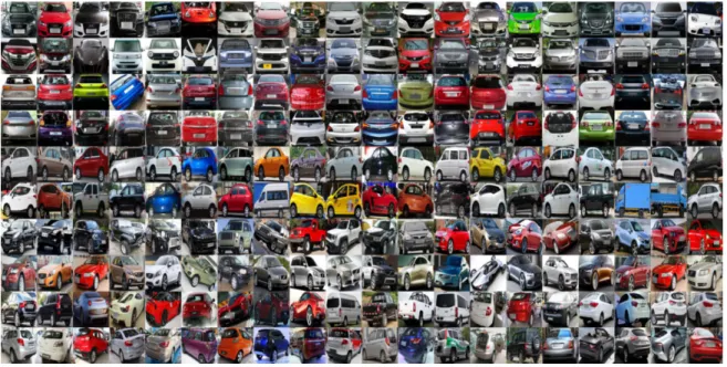
2.7 Example images of the web-nature data from the CompCars dataset. . . 29

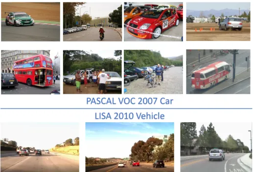
2.8 The upper images are examples from the PASCAl VOC 2007 Car dataset, while the bottom ones are from the LISA Vehicle Detection dataset. . . 30

2.9 Example images of different vehicle models from the VehicleID dataset. . . 31

2.10 A glance of the VeRi-776 dataset. Each vehicle is captured by more than 2 cameras in a city area. . . 31

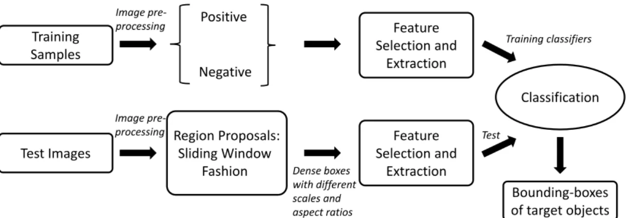
3.1 A general framework for conventional object detection methods. . . 35

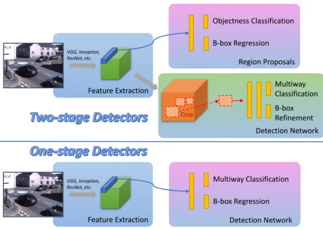
3.2 Deep learning models for object detection, which can be categorized into two-stage and one-stage frameworks. . . 36

(14)

3.3 The left sub figure is Restricted Boltzmann Machine (RBM) and the right

one is the Deep Belief Network (DBN) which is stacked by RBMs. . . 40

3.4 Kernels of DTCWT at different orientations: −5π/12,−π/4,−π/12,π/12,

π/4, and 5π/12, from left to right. . . 41

3.5 Multi-level complex wavelet feature extraction. . . 42

3.6 Results of hierarchical GMM clustering. Two clusters merge first if they

have similar viewpoints. . . 44

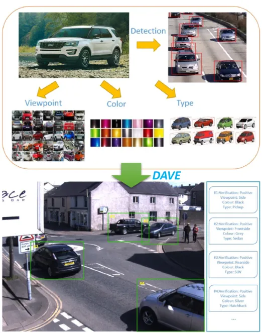
3.7 Illustration of DAVE. A vehicle has many semantic attributes that can be

applied to intelligent transportation systems, as shown in the upper sub-figure. Given numerous surveillance videos, human labeling is expensive and time-consuming. The motivation of our proposed DAVE is to annotate the location,

pose, type and color of all the vehicles on the raw videos automatically. . . 46

3.8 Training Architecture of DAVE. The FVPN is a shallow fully

convolu-tional network, which aims to precisely localize all the vehicles in real-time. The ALN is built by adding 4 fully-connected layers to extend the deep GoogLeNet into a multi-attribute learning model. These two networks are simultaneously optimized in a joint manner by bridging them with latent

data-driven knowledge guidance. . . 48

3.9 (a) Training data (columns indicate vehicle types, while rows indicate poses

and colors), (b) Training loss with/without knowledge learning. . . 51

3.10 A two-stage inference phase of DAVE. Vehicle candidates are first obtained from FVPN in real-time. Afterwards, we use ALN to verify each detection

and annotate each positive one with the vehicle pose, color and type. . . 54

3.11 Precision-recall curves on three vehicle datasets. FVPN+veri illustrates the detection results after verification by the ALN. MDPM-w/o-BB and MDPM-w-BB denote Mixture-DPM without / with bounding-box prediction,

respectively. . . 56

3.12 Examples of successful and failure cases for detection. A green box denotes correct localization, a red box denotes false alarm and a blue box denotes

missing detection. . . 58

3.13 Error analysis for detection results on VOC2007 car dataset. It shows the

false positive detections are mainly due to the incorrect localization. . . 58

3.14 Qualitative results of attributes annotation. Red marks denote incorrect

annotation, and N/A(C) means a catch-all color. . . 62

4.1 Comparison of vehicle and person re-ID. The variation of visual pattern

(15)

List of figures xv

4.2 A sketch of our proposed multi-view vehicle re-ID framework. Cross-view

images are generated based on the input image, thus distance metric learning can be conducted on the viewpoint-invariant multi-view feature space rather

than the single-view one. . . 68

4.3 An overview of the SCCN. We aim to infer multiple viewpoints’ images of a

vehicle from only one visible view and exploit their feature maps to learn the

final re-ID model. . . 71

4.4 An overview of the architecture of SCCN which consists of two sub-networks

shaded in the color of orange and pink. The first part employs nine parallel sets of convolutional and deconvolutional layers to infer transformations between the input visible view and other hidden views of a vehicle. Training

the spatially concatenatedDeconv1_concat layer is first supervised by two

kinds of ground truth label matrices shaded in the color of green, which are

All_View_ImageandViewpoint_Label_Matrixfor regression and classifi-cation, respectively. The second sub-network further adopts convolutional and fully-connected layers to learn non-linear mappings from the concate-nated feature maps to a global multi-view feature representation of the input

vehicle. (Better viewed in color.) . . . 73

4.5 Collection of the Toy Car RE-ID Dataset. Three angles 30◦, 60◦and 90◦, and

50 views in each angle are available to be used. The picture at the bottom

gives a glance of the final synthesized data in angle 30◦with 8 views for each

vehicle. . . 77

4.6 Visualization examples of theConv_f c_reginference. Row A1 and B1 show

samples inferred from the only one input view. TheAll_View_Imageground

truths are compared in Row B1 and B2. . . 80

4.7 t-SNE demonstration of multi-view features compared with single-view

features of samples from 50 test vehicles in the VeRi dataset. It shows our

learned multi-view features are more viewpoint-invariant. . . 81

4.8 Examples of illumination synthesis on three different levels. . . 83

4.9 CMC curves comparisons of different re-ID methods on the Toy Car RE-ID,

(16)

4.10 (a)Overview of the proposed XVGAN. A Classification Net is first used for learning vehicles’ intrinsic features containing model, color and type information. Besides, viewpoint features are also learned. The Generative Net then takes a vehicle’s intrinsic feature of the visible view, the average feature of the expected viewpoint and a random noise vector as inputs to infer images of the same vehicle in other views. The Discriminative Net distinguishes real images from synthetic samples while keeping images generated with correct vehicle attributes. Finally, the inferred vehicle images from cross-view pair data contribute to learning distance metrics for re-ID.

(b)Generated image examples in different viewpoints for the input vehicle. 86

4.11 Network Architecture of the XVGAN. The yellow part is for learning the central features of five main viewpoints by k-means clustering. The Discrim-inative Net is not only for generative adversarial training but also supervised by vehicles’ multi-attributes to help the Generative Net infer real images with correct vehicle attributes in certain views. The final convolutional layers in the Classification Net and the Discriminative Net are concatenated in depth

for further learning to measure distances by contrastive loss. . . 89

4.12 Qualitative examples of generated vehicle images in different viewpoints from only one original visible view. The left column shows the original vehicle images and their corresponding ground truths in five viewpoints. The right four columns show generated samples by VAE, Attributes-conditioned

GAN, XVGAN without matching-awareness and XVGAN. . . 94

4.13 CMC results evaluated on the VeRi dataset. The solid lines denote image generation models, while the dashed lines are methods only exploiting the

original one view. . . 96

4.14 Qualitative success and failure examples of top-20 rank on the VeRi dataset.

Green boxes mean correct hits, while red boxes denote wrong ones. . . 96

4.15 CMC results evaluated on the VehicleID dataset. The solid lines denote image generation models, while the dashed lines are methods only exploiting

the original one view. . . 97

5.1 Main components of our approach: The CNN extracts input vehicle image’s

feature. The LSTM-G infers multi-view features from only one input view. The LSTM-D discriminates whether the multi-view features are real or generated. A Siamese architecture is also built for learning distance metrics, given a vehicle image pair. . . 103

(17)

List of figures xvii

5.2 An overview of the architecture of ABLN. The left part is a CNN for learning

input vehicles’ model and viewpoint features. The LSTM-G module aims to learn feature transformations between the input view and other invisible views. We design three different losses to learn these transformations. The first one is to adopt all the different viewpoint features of the input

vehi-cle as supervision information to optimize a reconstruction loss LReconst.

Additionally, we build another LSTM-D module to discriminate the real different view features and the inferred ones. The two LSTM modules can be

optimized as a generator and a discriminator by an adversarial lossL_Advers.

Moreover, given an image pair, a re-ID lossL_Reid is configured at the end of

the LSTM-G for distance metric learning. Note that both the LSTM-G and LSTM-D are bi-directional. . . 105

5.3 Details of the unwrapped LSTM-G module. At each view step of the LSTM

unit, the input is a feature vector concatenated by the feature of the input view and the average viewpoint feature of that certain view. The outputs are supervised by the features of the corresponding views of the input vehicle using a cross-entropy loss. . . 106

5.4 CMC results of models trained by a different number of inferred views. (a)

Comparisons on the VeRi dataset. (b) Comparisons on the VehicleID dataset. 111

5.5 Qualitative top-10 rank comparisons of the ABLN-V trained by a differentV

number of inferred views. Blue boxes are query vehicles, while the green and red boxes denote correct hits and wrong ones, respectively. The right part visualizes the single-view features obtained by the ABLN-0 without any viewpoint inference and the multi-view features inferred by the ABLN-32. . 112

5.6 Visualization of the output feature space at different view steps of the LSTM-G.114

5.7 Comparisons of CMC curves with state-of-the-arts. (a) Results on the VeRi

(18)

5.8 An overview of the architecture of VAMI. TheF Net is for learning single-view features containing vehicles’ intrinsic information such as model, color and type. Moreover, viewpoint features can be also learned so that the central point feature of each viewpoint cluster over the whole training set can be obtained and used for attention learning. The attention model aims to output viewpoint-aware attention maps from the input view image targeting at different viewpoints. To infer multi-view features from the obtained attentive single-view features, we design a conditional generative network trained by an adversarial architecture. The networks of the real data branch are only available in the training phase. Auxiliary vehicle classifiers are configured

at the end ofDto help match the inferred multi-view features with correct

input vehicles’ identities. Finally, given positive and negative vehicle pairs, a contrastive loss is designed to optimize the network for distance metric

learning. (Best viewed in color.) . . . 118

5.9 The details of the viewpoint-aware attention model. The top-right part gives examples of overlapped regions of certain arbitrary viewpoint pairs. . . 120

5.10 Viewpoint-aware attention maps. The upper row shows the input images and the bottom row shows the output attention maps. The highly-responded region is obtained by the input view attended with the central viewpoint feature of the target viewpoint. . . 124

5.11 The left part compares qualitative results (Top-10 ranks) of single-view feature+L_Reid and our VAMI. Blue boxes are query vehicles, while the green and red boxes denote correct hits and incorrect ones, respectively. The right part visualizes the spaces of the original single-view features and the multi-view features inferred by our VAMI. . . 125

5.12 (a) CMC results of evaluation of the multi-view inference. (b) CMC results of studies of the adversarial structure. . . 126

6.1 The general framework to address the image captioning task. . . 136

A.1 The architecture of AlexNet [76]. . . 151

A.2 The architecture of VGGNet [128]. . . 152

A.3 The architecture of the first version GoogLeNet [135]. . . 153

A.4 Residual learning: a building block. [58]. . . 154

(19)

List of tables

2.1 Comparisons of different general object detection methods. . . 18

3.1 Comparisons of different methods on average precision and computational time. . . 45

3.2 Vehicle detection AP (%) and speed (fps) comparison on the UTS, PASCAL VOC2007 and LISA 2010 datasets . . . 56

3.3 Evaluation (%) of attributes annotation compared to one-net pipeline on the UTS dataset . . . 60

3.4 Evaluation (%) of attributes annotation for vehicles on the UTS dataset . . . 61

3.5 Evaluation (%) of fine-grained vehicle type classification on the UTS dataset 61 4.1 Parameter settings of the SCCN. Leaky-ReLU activation is set after each convolutional and fully-connected layer. . . 74

4.2 Evaluation (%) of effectiveness of each component proposed in the SCCN. The left part studies the proposed multi-view inference. The right part studies the architecture of the SCCN. . . 79

4.3 Rank-1 rate (%) of Data Augmentation by Illumination Synthesis. . . 82

4.4 Comparisons (%) with state-of-the-art re-ID methods. . . 84

4.5 Evaluation (%) on the VeRi dataset. . . 85

4.6 mAP and matching rate (%) at rank-1, 5, 20 and 50 on VeRi Dataset. Attr-GAN denotes Attribute-conditioned Attr-GAN, and w/o-M is abbreviation of without Matching-awareness. XVGAN-C only adopts the feature in the Classification Net. . . 95

4.7 Matching accuracies (%) at rank-1, 5, 20 and 50 on the two-view VehicleID Dataset. . . 97

(20)

5.2 Comparisons (%) of bi/single-directional LSTM. ASLN is the abbreviation of Adversarial Single-directional LSTM Network. The number of inferred views is fixed as 32. . . 113

5.3 Comparisons (%) of dropping different losses. The number of inferred views

is fixed as 32. . . 113

5.4 Comparisons (%) of our method with state-of-the-arts. . . 115

5.5 Evaluation (%) of effectiveness of the multi-view inference (MV Infer.) and

adversarial network (Advers. Net.). . . 125

5.6 Evaluation (%) of attention model. k is the number of the attention step. n is

the noise rate in the form of dropout. . . 127

5.7 Comparisons (%) with state-of-the-art re-ID methods. Methods in the last

(21)

Chapter 1

Introduction

1.1

Vision-based Intelligent Transportation Systems

Intelligent transportation systems (ITS) are defined as the systems exploiting techniques of sensing, analysis, control, and communications to ground transportation so as to develop and improve mobility, efficiency and security. ITS contains a wide range of applications [130, 9] that process and transmit data to mitigate traffic congestion, benefit traffic management and improve rapid responses to emergent accidents.

Video surveillance is one of the main branches in public transportation systems and has a huge potential to be researched since it contributes to the planning and control of the traffic networks. With the ever-increasing number of vehicles in the world, the exploration of advanced intelligent algorithms becomes more important and imperative. Previously, observing and analyzing video data requires large manpower, which is highly inefficient. However, in the past decade, the decreasing costs of surveillance cameras make huge traffic data recorded and available to be utilized. There have been many computer vision methods developed to analyze video surveillance data.

In urban traffic systems, certain surveillance tasks such as vehicle counting [6], license plate recognition [14] and incident detection [28], can be addressed either by sensor-based or vision-based algorithms. However, vision-based methods can fully take advantages of the abundant visual patterns to recognize target objects in a human-like way. Take the application of vehicle detection as an example, the radar sensor-based techniques can only detect vehicles in a very limited area, while the vision-based approaches can find all the vehicles in a large visible area by a camera and describe additional features of each detected vehicle simultaneously. Therefore, in this thesis, several computer vision and machine learning models are presented and extensively studied to address a variety of interesting tasks in the intelligent transportation systems.

(22)

1.2

Visual Feature Learning

In this section, an overview of deep learning for computer vision is introduced. Before talking about deep visual feature learning, we first revisit the traditional machine learning approaches. In pattern recognition problems, most of the previous efforts can be grouped into extracting robust features and learning discriminative classifiers. Feature representation is always the key to recent progress in various computer vision tasks. A conventional recognition framework can be illustrated in Figure 1.1. Given input image data, carefully designed hand-crafted features based on domain knowledge are first extracted, which do not require learning in task-specific models. Such features are low-level representations directly computed from the pixel values of images, and usually difficult and expensive to design to make machine learning algorithms work. There have been many successful low-level visual features such as SIFT [101], HOG [24], SURF [7], MSER [106], LBP [2] and GLOH [107]. Once the feature extraction is completed, traditional machine learning methods are performed for classification or regression. Among numerous approaches, linear regression, logistic regression, Bayes classification [35], decision tree [116], k-Nearest Neighbor [53], support vector machine (SVM) [52] and Adaptive Boosting (AdaBoost) [141] are the most widely adopted ones in computer vision tasks.

Fig. 1.1 A traditional framework for addressing pattern recognition tasks, which mainly consists of hand-crafted feature extraction and learning classifiers.

The concept of deep learning is not novel, which has been around for a couple of years now. But nowadays with the available big data and the powerful computing ability by the parallel computing platform and programming model CUDA, deep learning is getting

(23)

1.2 Visual Feature Learning 3

more attention and has achieved great success in many vision applications such as image classification [76, 128, 135], retrieval[142], segmentation[100] and object detection[38, 37]. Deep learning has two main research branches. One is the convolutional neural networks (CNNs) for addressing tasks in computer vision while the other is recurrent neural networks (RNNs) designed mainly for natural language processing. CNN is initially proposed for learning hierarchical visual features of images, where one layer extracts features from the output of its previous layer. A schematic diagram is shown in Figure 1.2. A deep CNN contains an input and an output layer as well as multiple hidden layers which usually consist of several convolutional layers, pooling layers, fully-connected layers and normalization layers. Each hidden layer is desired to learn a different level representation. For example, assume a deep network configured with three hidden layers, the first layer would learn the edge features, while the second and third layer could extract object parts’ and objects’ representations, respectively. Moreover, RNN is a class of neural network where connections between units form a directed cycle. This allows it to exhibit dynamic temporal behavior. Unlike forward neural network, RNNs can use their internal memory to process arbitrary sequences of inputs.

Feature maps

Feature maps Feature maps Input image

Fig. 1.2 A simple deep ConvNet for image classification.

Now we consider the approaches of learning features which can be coarsely categorized into supervised learning and unsupervised learning. The majority of practical machine learning adopts supervised learning. Supervised learning is where you have input variables

x and an output variable y, and then design an algorithm to learn the mapping function

from the input to the output. The goal is to approximate the mapping function so well

that when you have new test dataxthat you can predict the output variablesyfor that data.

Some popular examples of supervised learning algorithms are the linear regression [124] for regression problems, random forest [8] for classification and regression problems, SVM [22] for classification problems. On the other side, unsupervised learning is where you only

(24)

have input dataxand no corresponding output variables. The goal for unsupervised learning is to model the underlying structure or distribution in the data in order to learn more about the data. Unsupervised learning problems can be further grouped into clustering [48] and association problems [115].

Deep neural networks can be trained in an unsupervised or supervised manner for both unsupervised and supervised learning tasks. In the supervised learning, end-to-end learning of deep architectures with back-propagation is the most preferred framework. It works well when the amount of labels is large. The structure of the model is important as well. Deep neural network, convolutional neural network and recurrent neural network all have successful examples in supervised learning. Besides, deep unsupervised learning adopts layer-wise training to learn statistical structure or dependencies of the unlabeled data. Some popular examples are deep stacked denoising autoencoder [139], deep belief nets [61] and hierarchical sparse coding [66].

1.3

Object Detection

In computer vision, classification is the most well-known research topic which aims to classify an image into one of many different categories. Different from classification, localization finds the location of a single object inside the image. Iterating over the problem of localization plus classification we end up with the need for detecting and classifying multiple objects at the same time. Object detection is the problem of finding and classifying a variable number of objects on an image, which is shown in Figure 1.3.

(25)

1.4 Object Re-identification 5

Object detection is usually considered as the most fundamental task in computer vision, which encounters many challenges. The first one is the variable number of objects. When training machine learning models, we need to represent data into fixed-size vectors. Since the number of objects in the image is not known beforehand, we would not know the correct number of outputs. Historically, the variable number of outputs has been tackled using a sliding window based approach, generating the fixed-size features of that window for all the different positions of it. After getting all predictions, some are discarded and some are merged to get the final result. Another severe challenge is the different conceivable scales of objects. When doing simple classification, only objects that cover most of the image are needed to be classified. However, to detect certain objects as small as a dozen pixels (or a small percentage of the original image), traditional sliding window fashions are highly inefficient. Various other difficulties are illumination change, viewpoint variation, and deformation problems.

The most two popular classic object detection approaches are the Viola-Jones framework [141] and the deformable part models (DPM) [32]. The Viola-Jones method works by generating different simple binary classifiers using Haar features. These classifiers are assessed with a multi-scale sliding window in cascade and dropped early in case of a negative classification. The DPM method uses a histogram of oriented gradients (HOG) feature and SVM for classification. Recently, deep learning detectors combine feature learning and classifier training together to achieve satisfied performance with both the high precision and fast processing speed. In this thesis, we propose a deep CNN-based vehicle detector which has reached a superior performance over state-of-the-art methods.

1.4

Object Re-identification

Object re-identification (re-ID) is the task of recognizing an object, captured by one or more cameras, over a range of candidates targets. The re-ID problem is initially proposed to target on persons, and then extended to vehicles recently. Take vehicle re-ID as an example, the main issues are due to the fact that the same vehicle is usually acquired at different times and by different disjoint cameras. Object re-ID can be considered as a sub-area of image retrieval, dealing with matching images of the same object over multiple non-overlapping camera views.

Re-ID techniques are applicable in tracking a particular object across different cameras, tracking the long-term trajectory of a target object in surveillance, and for forensic and security applications. First, multi-camera tracking is to track an individual using multiple cameras, the identity of the object has to be retrieved from the second camera based on

(26)

the information obtained from the first camera. Second, if the locations of the cameras are known, based on the re-ID system, it is possible to track the moving path of an object from one point to another. Moreover, in surveillance and security applications, re-ID models can be employed to track the suspect in a crime scene.

At present, there are still some of the major challenges for the re-ID system being addressed in the computer vision community. Figure 1.4 gives some examples of images in a person re-ID dataset. First, illumination change causes the variation in the appeared color of the same subject across multiple cameras. As many of the older surveillance cameras give low-resolution images, it is a difficult task for the algorithm to differentiate between individuals due to the lack of appearance details. In crowded scenes, the partial or full occlusion will also severely decrease the performance. Moreover, obtaining the data for re-ID is easy, but annotated data is always scarce. For good generalization capabilities, complex algorithms need to be taught with a large number of labeled data.

Fig. 1.4 Some examples from the VIPeR [46] dataset for exploring person re-ID. Each pair of images are two shots of one person identity captured from different cameras.

Most existing re-ID approaches are carried out focusing on two aspects of the problem. To develop a mathematical representation for the images, known as a feature representation, and to develop a distance function that can reduce the distance between samples of the same

identity and increase the distance between samples of different identities in ann-dimensional

(27)

1.5 Thesis Outline 7

1.5

Thesis Outline

The rest of the thesis is structured as follows.

Chapter 2 contains a full literature review of some representative previous works relevant to deep visual feature learning. The basics of convolutional neural networks and recurrent neural networks are mainly reviewed as well as their corresponding applications. Then, object detection approaches including traditional detection frameworks and deep learning based detectors are studied. Vehicle detection methods are specifically reviewed in a subsec-tion. Moreover, works related to object re-identification targeting at person and vehicle are separately reviewed. Various other topics that are relevant to this thesis are also considered. Generative Adversarial Networks (GANs) achieve great success on image generation tasks because the adversarial learning forces the generated samples to be indistinguishable from real data. Visual attention mechanisms aim to automatically focus on the core regions of im-age inputs and ignore the useless parts. Finally, some main datasets used in our experiments and evaluation protocols are introduced.

Chapter 3 studies deep neural networks for vehicle detection and multi-task learning. It first presents a simple model using multi-level complex wavelet feature representations and deep belief neural network for training a vehicle detector. Then, a vehicle detection and annotation method DAVE, which consists of two convolutional neural networks, are proposed to jointly address vehicle detection and attributes prediction via multi-task learning.

In Chapter 4, two models for addressing vehicle re-identification via generating cross-view images are investigated. First, we present a spatially concatenated ConvNet (SCCN) to learn transformations across different viewpoint pairs of a vehicle separately in a convolutional encoder-decoder architecture, and then spatially concatenate all the feature maps and map them into a global feature for learning the distance metrics. Moreover, a novel deep cross-view generative adversarial network (XVGAN) is proposed for generating cross-cross-view vehicle images from an input view. Through experiments, the model is extended to benefit the multi-view vehicle re-ID task.

Chapter 5 extends the works of Chapter 4 from image-level generation to feature-level transformation learning. The uncertainty of vehicle viewpoint in re-ID is still our research point. An adversarial bi-directional LSTM network (ABLN) is proposed to exploit the great advantages of the Long Short-Term Memory (LSTM) to model transformations across continuous view variation of a vehicle and adopts the adversarial architecture to enhance training. Moreover, we research the visual attention mechanism and design a viewpoint-aware attentive multi-view inference (VAMI) model. A viewpoint-viewpoint-aware attention model is proposed to obtain attention maps from the input image. The high-scored region of each map shows the overlapped appearance between the input vehicle’s view and a target viewpoint.

(28)

Given the attentive features of a single-view input, a conditional multi-view generative network is designed to infer a global feature containing different viewpoints’ information of the input vehicle. The adversarial training mechanism and auxiliary vehicle attribute classifiers are combined to achieve effective feature generation.

(29)

Chapter 2

Literature Review

2.1

Deep Visual Feature Learning

2.1.1

Convolutional Neural Network

Convolutional Neural Network (CNN) [82] is an important tool for most machine learning practitioners today. A CNN model usually consists of one or more convolutional layers (often with a sub-sampling step) followed by one or more fully-connected layers as in a standard multi-layer neural network. The architecture of a CNN is designed to take advantage of the 2D structure of an input image, which is achieved with local connections and tied weights followed by some form of pooling which results in translation invariant features. Another benefit of CNNs is that they are easier to train and have much fewer parameters than fully-connected networks with the same number of hidden units. In the following sub-sections, the main operations in a general CNN model are introduced individually. Convolution

The initial layers that receive an input signal are called convolution filters. Convolution is a process where the network tries to label the input signal by referring to what it has learned in the past. If the input signal looks like previous cat images it has seen before, the “cat” reference signal will be mixed into, or convolved with, the input signal. The resulting output signal is then passed on to the next layer. A more intuitive schematic diagram of the convolution operation is demonstrated in Figure 2.1.

Convolution has the nice property of being translational invariant. Intuitively, this means that each convolution filter represents a feature of interest (e.g whiskers, fur), and the CNN algorithm learns which features comprise the resulting reference (i.e. cat). The output signal

(30)

*

=

4

Fig. 2.1 The convolution operation. The filters are convolved over a feature map in a sliding window fashion.

strength is not dependent on where the features are located, but simply whether the features are present. Hence, a cat could be sitting in different positions, and the CNN algorithm would still be able to recognize it. Moreover, we need to specify other important parameters such as the channel depth, stride, and zero-padding. The channel depth corresponds to the number of filters we use for the convolution operation. The more filters we have, the more image features get extracted and the better our network becomes at recognizing patterns in unseen images. Stride is the number of pixels by which we slide our filter matrix over the input matrix. When the stride is 1 then we move the filters one pixel at a time. When the stride is 2, then the filters jump 2 pixels at a time as we slide them around. Having a larger stride will produce smaller feature maps. Sometimes, it is convenient to pad the input matrix with zeros around the border, so that we can apply the filter to bordering elements of our input image matrix. A useful feature of zero padding is that it allows us to control the size of the feature maps.

Non Linearity Activation

The activation layer controls how the signal flows from one layer to the next, emulating how neurons are fired in the network. Output signals which are strongly associated with past references would activate more neurons, enabling signals to be propagated more efficiently for identification. CNN is compatible with a wide variety of complex activation functions to model signal propagation, the most common function being the Rectified Linear Unit (ReLU), which is favored for its faster training speed. Its output is given by:

(31)

2.1 Deep Visual Feature Learning 11

ReLU is an element-wise operation (applied per pixel) and replaces all negative pixel values in the feature map by zero. The purpose of ReLU is to introduce non-linearity in the CNN model since most of the real-world data we would want the network to learn would be non-linear (Convolution is a non-linear operation - element-wise matrix multiplication and addition, so we account for non-linearity by introducing a non-linear function like ReLU).

Pooling or Sub-sampling

Inputs from the convolutional layer can be “smoothed" to reduce the sensitivity of the filters to noise and translation variations. This smoothing process is called pooling or sub-sampling and can be achieved by taking averages or taking the maximum over a sample of the signal. Such spatial pooling reduces the dimensionality of each feature map but retains the most important information. In case of max pooling shown in Figure 2.2, we define a spatial

neighborhood with a 2×2 window and take the largest element from the rectified feature

map within that window. Instead of taking the largest element, the average (average pooling) or the sum of all elements can be computed in that window. In practice, max pooling has been shown to obtain better performance.

Fig. 2.2 The max pooling operation.

Fully-Connected Layer

The last layers in the network are usually fully-connected, meaning that neurons of preceding layers are connected to every neuron in subsequent layers. The output from the convolutional and pooling layers represent high-level features of the input image. The purpose of the Fully-Connected layer is to use these features for classifying the input image into various

(32)

classes based on the training dataset. Apart from classification, adding a fully-connected layer is also a cheap way of learning non-linear combinations of these features. Most of the features from convolutional and pooling layers may be good for the classification task, but combinations of those features might be even better.

Back Propagation

The training process of a CNN model is generally based on the back propagation algorithm [121]. Use back propagation to calculate the gradients of the error with respect to all weights in the network and use gradient descent to update all filter weights and parameter values to minimize the output error. First, the forward propagation can be generalized as that given the

activatedl-th layeral, the(l+1)-th layer’s activation is computed as:

zl+1=Wlal+bl, (2.2)

al+1= f(zl+1).

The error term for the (l+1)-th layer is defined as δl+1. The loss function is set as

L(W,b;x,y) where(W,b) are the parameters and (x,y) are the training data and label

pairs. If thel-th layer is densely connected to the(l+1)-th, then the error for thel-th layer

is computed as:

δl= ((Wl)Tδl+1)·f′(zl), (2.3)

Where “·” denotes the element-wise product operator. Then, the gradients are:

∇_WlL(W,b;x,y) =δl+1(al)T, (2.4)

∇_blL(W,b;x,y) =δl+1.

If thel-th layer is a convolutional and pooling layer then the error is propagated through as:

δ_kl=upsample((Wl_k)Tδ_kl+1)·f′(zl_k), (2.5)

Wherekindexes the filter number and f′(zl_k)is the derivative of the activation function. The

upsample operation has to propagate the error through the pooling layer by calculating the error with respect to each unit incoming to the pooling layer. Finally, to calculate the gradient

(33)

with respect to the filter maps, we rely on the border handling convolution operation again

and flip the error matrixδ_kl the same way we flip the filters in the convolutional layer.

∇_Wl kL(W,b;x,y) = m

∑

i=1 (al_i)∗rot90(δ_kl+1,2), (2.6) ∇_bl kL(W,b;x,y) =

∑

c,d (δ_kl+1)c,d.

Wherealdenotes thel-th layer’s input.(al_i)∗δ_kl+1is the convolution between thei-th input

in thel-th layer and the error with respect to thek-th kernel filter. mis the number of input

channels. rot90(A,2)is the function to rotate inputAby 90×2 degrees in anti-clockwise

direction. Moreover,candd are the width and height of the kernel filter, respectively.

Common Loss Functions

In machine learning, optimization is usually driven by a loss function which specifies the goal of learning by mapping parameter settings to a scalar value specifying the“badness” of these parameter settings. The goal of learning is to find a setting of weights that minimizes the loss functions. Some common loss functions adopted to train deep neural networks are

briefly explained as follows, where N andK denotes the number of training samples and

classes, respectively.

Euclidean Lossis also known asℓ2loss defined as: E = 1 2N N

∑

n=1 ||yˆn−yn||2₂. (2.7)

This can be usually adopted to learn least-square regression tasks.

Information Gain Losstakes an “information gain” matrix specifying the “value” of all label pairs and is defined as:

∀n K

∑

k=1 ˆ p_nk=1, (2.8) E(pˆn) = −1 N N

∑

n=1 K

∑

k=1 H_l_n,klog ˆpn,k.

WhereH_l_n denotes row lnof H and ln∈[0,1,2, ...,K−1]indicates the correct class label

among theKclasses. IfH is the identity matrix, this is equivalent to the multinomial logistic

(34)

Softmax Losscomputes the multinomial logistic loss for a one-of-many classification task, passing real-valued predictions through a softmax to get a probability distribution over classes. Its definition will be further explored in Eq. 3.4.

Dropout Operation

Dropout operation is another important concept used in training a deep model. Dropout refers to ignoring neurons during the training phase of certain set of neurons which is chosen at random. “Ignoring” means these units are not considered during a particular forward or backward pass. At each training stage, individual nodes are either dropped out of the net

with probability 1−por kept with probabilityp, so that a reduced network is left. Dropout

aims to prevent over-fitting, since a fully-connected layer occupies most of the parameters, and hence, neurons develop co-dependency amongst each other during training which curbs the individual power of each neuron leading to over-fitting of training data.

2.1.2

Recurrent Neural Network

Recurrent neural networks (RNNs) [93] have a general architecture illustrated in Figure 2.3. This chain-like nature reveals that RNNs are intimately related to sequences and lists. The natural architecture of neural network is appropriate to use for such data. In the past five years, RNNs have been successfully applied to a variety of problems: action recognition [95, 96], image captioning [150], language modeling [45], etc. In the following sub-sections, the vanilla RNN and its variants are reviewed.

(35)

Vanilla RNN

For time sequence data, in addition to the current input, a hidden state representing the features in the previous time sequence also needs to be considered. For example, to make a

word prediction at time stept in image captioning, both the inputXt and the hidden state

from the previous time stepht−1are used to computeht:

ht= f(Xt,ht−1). (2.9)

In RNN, h serves 2 purposes: the hidden state for the previous sequence data as well

as making a prediction. However, for modeling long sequence data, although RNN is theoretically able to learn the long-term dependencies, the performance is unsatisfactory in practice due to the vanishing gradient.

Long Short-Term Memory

Long Short-Term Memory networks (LSTMs) [62] aim to address learning long-term depen-dencies. In vanilla RNNs, each repeating module has a simple structure such as a single tanh

layer. LSTM splits theht in RNN into 2 separate variablesht andC. It contains three gates:

forget, input, and output, to control what information will pass through:

gate_{f orget} =σ(Wf xXt+Wf hht−1+bf), (2.10)

gate_input =σ(WixXt+Wihht−1+bi),

gate_{out put}=σ(WoxXt+Wohht−1+bo).

Where gate_{f orget} controls what part of the previous cell state will be remained, gate_input

controls what part of the new computed information will be added to the cell stateC, and

gate_{out put} controls what part of the cell state will be exposed as the hidden state. In addition,

σ(x) = (1+e−x)−1. Then, the cell state and the hidden state will be updated as:

e

C=tanh(WcxXt+Wchht−1+bc), (2.11)

Ct =gatef orget·Ct−1+gateinput·Ce, ht =gateout put·tanh(Ct).

Where the new stateCt is formed by forgetting part of the previous cell state while adding

(36)

what cell state to export asht. tanh(x) = e x₋_e−x

ex₊_e−x. An overall diagram of LSTM is shown in

Figure 2.4.

𝜎

𝑡𝑎𝑛ℎ

𝜎

𝑡𝑎𝑛ℎ

𝑋' ℎ'() ℎ' 𝑔𝑎𝑡𝑒,-./0' 𝑔𝑎𝑡𝑒3456' 𝐶2 𝐶'() 𝐶' 𝑔𝑎𝑡𝑒-6'56' 𝐶' ℎ'

Fig. 2.4 The architecture of Long Short-Term Memory.

Gated Recurrent Unit

Gated Recurrent Unit (GRU) [21] is a variant of the LSTM with a simpler structure, which combines the forget and input gates into a single “update gate”, and does not maintain a cell

stateC. Figure 2.5 illustrates its design.

𝜎

𝑡𝑎𝑛ℎ

1 −

𝑋

₎

ℎ

_)*+

ℎ

₎

𝑔𝑎𝑡𝑒

./01)2

ℎ3

₎

𝑔𝑎𝑡𝑒

4

(37)

2.2 Object Detection 17

gate_r=σ(WrxXt+Wrhht−1+br), (2.12)

gate_update=σ(WuxXt+Wuhht−1+bu).

The new hidden state is computed as:

e

ht=tanh(WhxXt+Whh·(gater·ht−1) +bh), (2.13)

ht= (1−gateupdate)·ht−1+gateupdate·he_t,

Where gate_r is used to control what part of ht−1 to compute a new proposal het. We use

gate_updateinstead of creating a new gate to control what we want to keep from theht−1.

2.2

Object Detection

2.2.1

Evaluation Metrics

In the computer vision research community, the task of object detection usually refers to predict the bounding-box of the target object. (Image segmentation and contour detection requires more fine-grained contour detection.) Intersection over Union (IoU) is an evaluation metric used to measure the accuracy of an object detector on a particular dataset. We often see this evaluation metric used in object detection challenges such as the popular PASCAL VOC challenge [29] and MSCOCO [92]. More formally, in order to apply IoU to evaluate an object detector, the ground truth bounding-boxes and the predicted bounding-boxes by a model are required. Computing IoU can, therefore, be determined as:

IoU= Area o f Overlap

Area o f U nion . (2.14)

Then, an IoU threshold can be specified to determine whether the localization is correct. Hence, each predicted box is either True Positive or False Positive. Each ground truth box is either True Positive or False Negative.

Precision (P) is defined as the number of True Positives (T_p) over the number of True

(38)

P= Tp

T_p+F_p. (2.15)

Recall (R) is defined as the number of True Positives (T_p) over the number of True

Positives plus the number of False Negatives (F_n).

R= Tp

Tp+Fn

. (2.16)

The precision-recall curve shows the tradeoff between precision and recall for different IoU threshold. A high area under the curve represents both high recall and high precision, where high precision relates to a low false positive rate, and high recall relates to a low false negative rate. Finally, the average precision is computed by averaging the precision values on the precision-recall curve where the recall is in the range [0, 0.1, ..., 1].

2.2.2

General Object Detectors

In this sub-section, we would like to review some classic general object detection approaches. A general comparison of different frameworks is listed in Table 2.1 and more details of pros and cons of each detector are explained in the following paragraphs.

Table 2.1 Comparisons of different general object detection methods.

Methods Deep / Non-Deep One / Two-Stage Region Proposal Mechanism Main Contribution

DPM [32] Non-Deep Two Sliding Window Mixtures of multi-scale deformable part models.

R-CNN [39] Deep Two Selective Search CNN + SVM

SPP-Net [57] Deep Two Selective Search Spatial pyramid pooling

Fast R-CNN [37] Deep Two Selective Search RoI pooling + multi-loss

Faster R-CNN [120] Deep Two Region Proposal Network RPN + Fast R-CNN

R-FCN [23] Deep One Sub-Region Position-sensitive score maps

SSD [97] Deep One Non-separate design Single-Shot

DPM [32]

Before the success of deep learning, the deformable part model (DPM) was the most popular object detector, which is proposed to represent highly variable objects using mixtures of multi-scale deformable part models. It aims at detecting objects that vary greatly in appearance and are hard to detect using rigid templates. The main idea of DPM is modeling different parts separately and introducing deformation cost to allow some variations of objects. The practical issues are considered to implement the model, such as the part filters are placed at

(39)

2.2 Object Detection 19

twice the spatial resolution of the placement of the root filters. To avoid elaborate labeling multiple parts, DPM treats the part locations as latent variables and uses latent SVM as the classifier. However, DPM is inefficient due to the sliding window fashion.

R-CNN [39]

Regions with CNN features are proposed by Girshick et al. and made a considerable

improvement of mean average precision (mAP) on the PASCAL VOC dataset. At the region proposals module, it uses selective search [138] to extract around 2000 category-independent region proposals. Then, R-CNN uses AlexNet to extract higher layer feature vectors such as FC-7 with 4096-dimensional feature vector. Finally, a multiple class SVM classifier is applied to evaluate the region proposal. A threshold of the score is learned to reject region proposals with low IoU overlap. Several region proposals recognized as positive might overlap and bound the same object, non-maximum suppression is used to merge them. SPP-Net [57]

R-CNN does improve the detection precision, but it has several notable drawbacks including training with multi-stage pipeline and feature caching which is expensive in time and space. Spatial pyramid pooling network (SPP-Net) proposed to speed up R-CNN by sharing compu-tation. SPP-Net is implemented via spatial pyramid pooling layer, but the back propagation through the SPP layer is highly inefficient when each training sample comes from a different image.

Fast R-CNN [37]

Fast R-CNN uses the idea of feature maps from SPP-Net, and integrates the training into a single-stage using a multi-task loss. Since it is single-stage training, no extra disk space for feature caching is required. A Fast R-CNN network has two sibling outputs, a discrete probability distribution (per Region of Interest) and bounding-box regression offsets for each object class. A joint loss is used to improve these two tasks performance together.

Faster R-CNN [120]

Faster R-CNN attempts to improve the region proposals generation by introducing a Region Proposal Network (RPN) which simultaneously predicts object bounds and objectness scores at each position. Once the region proposals are obtained, we feed them straight into what is essentially a Fast R-CNN. They add a pooling layer, some fully-connected layers, and finally

(40)

a softmax classification layer and bounding box regressor. In a sense, Faster R-CNN = RPN + Fast R-CNN.

R-FCN [23]

Region-based Fully Convolutional Net (R-FCN), shares 100% of the computations across every single output. The essential part of R-FCN is position-sensitive score maps. Each position-sensitive score map represents one relative position of one object class. In simple words, R-FCN considers each region proposal, divides it up into sub-regions, and iterates over the sub-regions asking: “does this look like the top-left of a baby?", “does this look like the top-center of a baby?", “does this look like the top-right of a baby?", etc. It repeats this for all possible classes. If enough of the sub-regions say“yes, I match up with that part of a baby!", the RoI gets classified as a baby after a softmax over all the classes.

SSD [97]

SSD stands for Single-Shot Detector, which provides enormous speed gains over Faster R-CNN. SSD performs the region proposal network and either fully-connected layers or position-sensitive convolutional layers in a “single shot", simultaneously predicting the bounding box and the class as it processes the image. It classifies and draws bounding-boxes from every single position in the image, using multiple different shapes, at several different scales.

2.2.3

Vehicle Detectors

Vehicle is one of most important targets in the object detection tasks. In addition to

gen-eral object detectors, there are also certain vehicle-specific detection methods. Sunet al.

[133] proposed to deploy HOG and Gabor features with SVM and neural network

classifica-tion. The experiments are evaluated on static images. Zhuet al. [175] designed dynamic

background modeling of overtake area, and performed validation on real-world video with ego-motion compensation. Moreover, Sivaraman and Trivedi [129] used Haar-like features with Adaboost classification and active learning algorithms to address vehicle detection.

Active learning has been shown to improve the detection and false alarm rates. Jazayeriet al.

[65] introduced a motion-based method which combines optical flow and hidden Markov model classification. The approach models the position and motion of preceding vehicles in the image plane.

(41)

2.3

Object Re-identification

2.3.1

Evaluation Metrics

In the task of re-identification (re-ID), the target objects’ images are usually cropped and aligned. The re-ID problem is similar to the instance retrieval task. Given one query image, the candidates with the same identity in the gallery set are desired to be placed in the top positions within a ranking list. To evaluate re-ID approaches, the cumulative matching characteristics (CMC) curve [144] is usually adopted by most of the researchers. In a CMC curve, the cumulative number of correctly matched queries is shown based on the ranking

list in which they have re-identified. When the number of true re-identified queries in ranki

isq(i), the CMC value for rankican be defined as:

CMC(i) =

i

∑

r=1

q(r). (2.17)

Wherer is the rank index. The advantage of CMC evaluation metric is that not only the

rank-1 is computed, but also the correctly matched queries in other top ranks can be indicated as well. Thus, CMC can better describe the re-ID performance of various methods.

Apart from CMC curves, if multiple ground truths for each query in the gallery set are available, mean average precision (mAP) [99] can be deployed to trade off the precision and recall to evaluate the overall performance for re-ID. Given an query image, the average precision (AP) can be defined as:

AP=∑

n

k=1P(k)×G(k)

Ngt

, (2.18)

WhereNgt denotes the number of ground truths, and nis the number of test tracks. P(k)

indicates the precision at cut-offkin the ranking lists. G(k)equals 1 when thek-th match is

true, otherwise 0. Thus, the mAP can be calculated over all queries as:

mAP= ∑

Q

q=1AP(q)

Q , (2.19)

(42)

2.3.2

Person Re-identification

Since most of the works have only explored the single image-based person re-ID problem, we mainly review such algorithms. To date, image-based methods can be coarsely categorized into three groups: image description, distance metric learning, and deeply-learned models. Feature Representation

Symmetry-Driven Accumulation of Local Features (SDALF) is proposed in [31] to extract three kinds of hand-crafted features on the symmetry-based silhouette. It includes the weighted color histograms, maximally stable color regions, and recurrent high-structured patches. The final feature matching is a weighted combination of distances computed by three feature representations. Gray and Tao [47] first partitioned a human image into horizontal stripes and adopted 8 color channels and 21 texture filters as local feature representations. A number of later works [168, 163, 15] introduced many enhanced hand-crafted features

but did not obtain large improvement. More recently, Liaoet al. [88] designed the local

maximal occurrence (LOMO) representation which consists of the color and Scale Invariant Local Ternary Pattern (SILTP [91]) histograms. The LOMO feature analyzes the horizontal occurrence of local features and performs maximization among sub-windows. LOMO feature has been successfully adopted in [159, 160] as the feature extraction part.

In addition to above low-level texture and color features, attribute-based mid-level representations have also been widely introduced in many state-of-the-art approaches. Layne

et al.[81] specified 15 semantic attributes such as shorts, sandals, and backpack, and adopted

low-level features to train attribute classifiers. Moreover, Zhao et al. [164] proposed a

method of learning mid-level filters to discover patch clusters. Such mid-level filters are discriminatively trained for identifying different visual patterns and distinguishing persons. To some extent, the method is invariant to cross-view variations.

Distance Metric Learning

Another significant research branch of person re-ID focus on distance metric learning whose basic idea is to put samples of the same identity together while pushing samples of different identities away. A general formulation is based on Mahalanobis distance function, which extends linear scalings and rotations of the space compared with normal Euclidean distance. The equation is defined as:

(43)

WhereMis a positive semi-definite matrix. (xi,xj)are pairwise data inputs. Large Margin

Nearest Neighbor (LMNN) [148] adopts an idea that a combination of allowance of slack for different classes (like SVMs) with the local region of a k-nearest neighbor sphere. The formulation tries to increase similarity to target neighbors while reducing it to impostors (other classes) lying within this k-nearest neighbor region. Information Theoretic Metric Learning (ITML) [25] formulates the problem as the minimization of differential relative entropy between two multi-variate Gaussian under constraints of the distance function. The tradeoff lies in satisfying constraints while being close to a prior (usually identity -leading to Euclidean distance). The constraints are to keep similar pairs below some distance

dsim and dissimilar pairs above ddi f f. Moreover, Logistic Discriminant Metric Learning

(LDML) is introduced in [50]. The probability of a pair being similar is modeled by a sigmoid function which includes a bias term, and the Mahalanobis distance, defined as

pi j=σ(b−d_M2 (xi,xj)). The metric is then estimated by gradient descent. KISSME [74] is a

non-iterative and extremely fast method to learn a metric. It assumes that the feature space of both hypothesis (pair is similar or dissimilar) is Gaussian, and then formulates the metric as

a difference of (inverted) covariance matrices, defined asMˆ =Σ−_y_{i j}1₌₁−Σ−_y_{i j}1₌₀, whereyi j =1

if a pair(i,j) is similar and 0 otherwise. Specifically,Σyi j=1=∑yi j=1(xi−xj)(xi−xj)

T _and Σyi j=0=∑yi j=0(xi−xj)(xi−xj)

T_{. They clip the spectrum of}_M_ˆ _{by eigenanalysis to obtain}

M. In their experiments, the assumption is satisfied by reducing the dimension of the features via PCA.

Aside from learning distance metrics, some researchers investigated subspace learning to

address person re-ID. Liaoet al.[88] proposed the cross-view quadratic discriminant model

to learn the projectionwto a low dimensional subspace as:

J((w) = w T_S bw wT_S ww , (2.21)

Where S_b and Sw indicates the inter-class and intra-class scatter matrices, respectively.

Furthermore, Zhanget al. [159] employed the null Foley-Sammon transform to optimize a

discriminative null space minimising the intra-class scatter and maximizing the inter-class scatter.

Deep Learning Models

Recently, deep learning models have largely benefited person re-ID, which hugely outperform previous methods

Deep Visual Feature Learning for Vehicle Detection, Recognition and Re-identification