Financial crises, unconventional monetary policy exit strategies, and agents' expectations

Financial Crises,

Unconventional Monetary

Policy Exit Strategies, and

Agents’ Expectations

Andrew T. Foerster

August 2011; Revised December 2011

RWP 11-04

Financial Crises, Unconventional Monetary

Policy Exit Strategies, and Agents’

Expectations

Andrew T. Foerster

Federal Reserve Bank of Kansas City

December 29, 2011

Abstract

A Markov switching DSGE model with …nancial frictions investi-gates the e¤ects of unconventional monetary policy (UMP) exit strate-gies. Agents in the model have rational expectations about the prob-ability of …nancial crises, the probprob-ability of a UMP response to crises, and the exit strategy used. Selling o¤ assets quickly produces a double-dip recession; in contrast, a slow unwind generates a smooth recovery. Increasing the probability of a UMP response to crises lowers pre-crisis consumption. The welfare bene…ts of increasing the probability of UMP may di¤er ex-ante versus ex-post, as can the preferred exit strategy.

The views expressed herein are solely those of the author and do not necessarily re‡ect

the views of the Federal Reserve Bank of Kansas City or the Federal Reserve System. I

thank Juan Rubio-Ramirez, Francesco Bianchi, Craig Burnside, Nobuhiro Kiyotaki, Eric Swanson, Stephanie Schmitt-Grohe, and Giuseppe Ferrero for helpful comments, as well as seminar participants at Duke, the Federal Reserve Banks of Richmond, Kansas City, and San Francisco, the Federal Reserve Board, Boston College, Michigan State, McMaster, the Bank of Canada, the 2011 International Conference on Computing in Economics and Finance, the 2011 North American Summer Meetings of the Econometric Society, and the "Conference on Zero Bound on Interest Rates and New Directions in Monetary Policy." Any remaining errors are my own.

y_{Research Department, Federal Reserve Bank of Kansas City, 1 Memorial Drive, Kansas}

1

Introduction

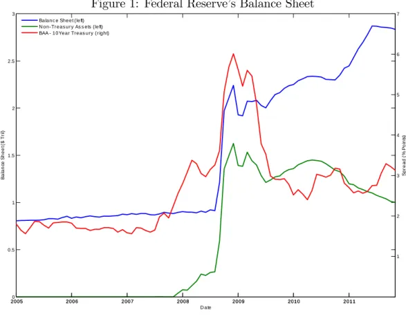
In the fall of 2008, the US economy experienced a …nancial crisis, marked by a deterioration in …nancial conditions along with a rapid slowing of real eco-nomic activity. In response, the Federal Reserve expanded its purchases of …nancial assets, injecting additional capital into the economy. The increased demand for …nancial assets provided by the Federal Reserve helped bolster asset values and alleviate the pressure on …nancial institutions by lessening the drop in the value of assets on their respective balance sheets. The Fed-eral Reserve accomplished this expansion in asset purchases by instituting a number of new lending facilities, such as expanding its purchases of mortgage backed securities and commercial paper. This response is deemed "uncon-ventional monetary policy" because of the wide range of assets purchased, in contrast to "conventional monetary policy" which typically consists of pur-chasing short-term Treasuries to manage short-term interest rates. In total, the value of non-Treasuries assets held by the Federal Reserve reached over $1.5 trillion. Figure 1 shows the sizeable increase in the total balance sheet, the non-Treasuries portion of the balance sheet, and a measure of interest rate spreads that jumped during the crisis, illustrating the increased level of uncertainty.

An additional feature of the …nancial crisis and Federal Reserve’s balance sheet expansion is that even after the crisis ended and interest rate spreads decreased from their peak, the size of the balance sheet remained elevated. In other words, the …nancial crisis triggered a start in unconventional monetary policy, but the end of the crisis did not trigger an end in unconventional policy. Rather than unwind its unconventional asset position as spreads decreased, the Federal Reserve maintained its asset position past the end of the crisis, and any exit strategy will be independent of the fall in spreads. Consequently, it remains to be seen how the Federal Reserve will unwind the its balance sheet, and what the e¤ects of this unwind are for the macroeconomy.

In addition to the issue of exit strategy, given that the Federal Reserve intervened with unconventional policy, one concern going forward is how

ex-pectations about intervention policy during crises a¤ect pre-crisis economic behavior. If economic agents expect the central bank to intervene during crises, this expectation may distort economic outcomes prior to a crisis occur-ring. During the crisis, concerns about the potentially negative repercussions of precedent-setting, such as reckless risk-taking, provided arguments against using unconventional policy. Even if intervention policy bene…ts the economy during crises, if setting a precedent of intervention has negative e¤ects during non-crisis times, it may be a poor policy choice to set this precedent. On the other hand, if expectations of intervention ease fears about small probability events and allow credit to ‡ow more freely, then setting a precedent may be an entirely positive policy choice.

Considering of the e¤ects of expectations along with the e¤ects during crises motivates an analysis of the welfare bene…ts of intervention policy. The main consideration with this welfare analysis is a form of time inconsistency:ex-ante

–that is, before a crisis occurs –making intervention more likely could decrease welfare, but ex-post –when a crisis occurs –making intervention more likely could improve welfare. In addition, choosing an exit strategy may depend upon the timing of the decision.

This paper addresses these questions about exit strategies, e¤ects of pre-crisis expectations, and welfare costs by building a dynamic stochastic general equilibrium (DSGE) model with a …nancial sector where …nancial crises occa-sionally occur, and conditional on a crisis occurring, the central bank may or may not intervene with unconventional policy. If the central bank does in-tervene, it will not do so forever, but at some point it will unwind its balance sheet, selling o¤ its accumulated assets at a speci…ed rate. Using Markov regime switching, the model allows agents to have rational expectations about transitions between regimes where the central bank intervenes and does not. This framework allows the study of exit strategies after intervention occurs, the e¤ects of expectations on pre-crisis economic activity, and the welfare gain or loss from di¤erent policy expectations.

There has been a rapidly growing literature on the implications of …nancial frictions in the macroeconomy. Many DSGE models, such as Christianoet al.

(2005) and Smets & Wouters (2007), do not incorporate a …nancial sector, and are therefore unable to explain movements associated with the banking system. A standard framework to incorporate a …nancial sector is to use a …nancial accelerator model, as developed in Bernanke & Gertler (1989), Kiy-otaki & Moore (1997), and Bernanke et al. (1999), which allows for frictions in the …nancial sector that slow the ‡ow of funds from households to …rms. Gertler & Karadi (2010) build upon the …nancial accelerator literature by in-corporating a central bank equipped unconventional monetary policy during crises, and show that intervention can lessen the magnitude of downturns as-sociated with …nancial crises. Other models that allow for …nancial frictions include Carlstrom (1997), Kiyotaki & Moore (2008), Brunnermeier & San-nikov (2011), Christianoet al. (2010), and Perri & Quadrini (2011). Shleifer & Vishny (2010), Cúrdia & Woodford (2010b), Cúrdia & Woodford (2010a), Cúrdia & Woodford (2011), Del Negroet al. (2010), Angeloni et al. (2011), Hilberg & Hollmayr (2011) consider government responses to crises or shocks in the presence of …nancial frictions.

Many of the papers that consider government intervention during …nancial crises lack the expectations and transitions between the intervention and no intervention regimes that are included in this paper. When expectations and transitions are ignored, any change in policy is entirely unexpected and consid-ered permanent. Therefore, without the regime switching introduced in this paper, the e¤ects of exit strategies and pre-crisis expectations have to be ig-nored as well. Following the rare event literature (Rietz (1988), Barro (2006), Barro (2009), and Gourio (2010)), this paper allows …nancial crises to occur with a small probability, and agents form expectations over the central bank’s decision to intervene conditional upon that rare even occurring. However, as in Barroet al. (2010), the model also allows crises to be persistent –that is, to last several periods before ending –and studies the implications of uncertain crisis duration. This uncertainty over crisis duration may have implications for the magnitude of the drop in real activity: if agents are uncertain about how long asset prices will remain suppressed, the economy may not rebound as quickly as if agents know that the crisis will be brief. Bianchi (2011) consider

the e¤ects of pre-crisis macroprudential policies, and Chari & Kehoe (2009) considerex-ante versus ex-post incentives of government bailouts.

Many recent papers use Markov switching to model expectations over dis-crete changes in government policy. Perhaps the most widely used appli-cation considers changing conventional monetary policy rules, such as Davig & Leeper (2007), Farmer et al. (2008), Farmer et al. (2009), and Bianchi (2010). With Markov switching, expectations over future policy rules a¤ect current dynamics of the economy. For example, in conventional monetary policy switching, expected changes in the in‡ation target or response to in‡a-tion can a¤ect current in‡ain‡a-tion. In this paper, the probability of changing to a regime where the central bank intervenes with unconventional policy can a¤ect pre-crisis dynamics, and expectations about exit strategies can a¤ect the initial portion of the crisis. Foerster et al. (2011) develop perturbation methods for Markov switching models, which allow ‡exibility in the modelling of the regime switching and allow for second-order approximations, which are important for welfare analysis.

The paper proceeds as follows. Section 2 discusses the model, with spe-cial emphasis on the …nanspe-cial sector. Section 3 details how the parameters of the economy change according to a Markov Process, and details the tran-sitions between regimes. The response of the economy to crises with and without intervention is discussed in Section 4, as are the e¤ects of di¤erent exit strategies. Section 5 analyzes the e¤ects of expectations of crisis poli-cies on the pre-crisis economy. Section 6 discusses the welfare implications of policy announcements, and Section 7 concludes.

2

Model

This section describes the basic model, based on that developed in Gertler & Karadi (2010). It is a standard DSGE model with the addition of a …nancial sector, which serves as an intermediary between households and non…nancial …rms. The next section describes the regime-switching in detail; this section simply notes which parameters switch.

2.1

Households

The economy is populated by a continuum of households of unit measure. These households consume, supply labor, and save by lending money to …nan-cial intermediaries or potentially to the government.

Each household is comprised of a fraction(1 f)of workers and a fraction

f of bankers. Each worker earns wages by supplying labor to non…nancial …rms, and each banker owns a …nancial intermediary that returns its earnings to the household. Bankers become workers with probability(1 ), so a total fraction of(1 )f transition to become workers; the same fraction transition from being workers to being bankers, and the probability is independent of duration. Upon exit, bankers transfer their accumulated net worth to the household, and new bankers receive initial funds from the household. Within the household, there is perfect consumption insurance.

The households maximize their lifetime utility function

E0 1 X t=0 t _{log (C} t hCt 1) { 1 +'L 1+' t (1)

where _E0 is the conditional expectations operator, 2 (0;1) is the discount

factor, Ct is household consumption at time t, h controls the degree of habit formation in consumption, Lt is household labor supply, { controls the disu-tility of labor, and' is the inverse of the Frisch labor supply elasticity.

Households earn income from workers earning a wage Wt on their labor suppliedLt, they receive an amount t of net pro…ts from …nancial and non…-nancial …rms, which equals pro…ts and banker earnings returned to the house-hold from exiting bankers less some start-up funds for new bankers, and they receive lump sum transfersTt. Households save by purchasing bondsBteither from …nancial intermediaries or the government, these bonds pay a gross real return ofRtin periodt+ 1. In equilibrium, both sources of bonds are riskless and hence identical from the household’s perspective, soRtis the risk-free rate of return. Households then have incomeRt 1Bt 1 from bonds. Consequently,

the household’s budget constraint is given by

Ct+Bt=WtLt+ t+Tt+Rt 1Bt 1. (2)

Using a multiplier %_t on (2), the household’s optimality conditions are

(Ct hCt 1) 1 h_Et(Ct+1 hCt) 1 =%_t; (3) RtEt %_t+1 %_t = 1; (4) {L'_t =%_tWt; (5)

which are for the marginal utility of conumption, bonds, and disutility of labor.

2.2

Financial Intermediaries

Financial intermediaries channel funds between the households and non…nan-cial …rms. Finannon…nan-cial intermediaries, indexed by j, accumulate net worth Nj;t and collect deposits from householdsBj;t. Using these two sources of funding, they purchase claims on non-…nancial …rms Sj;t at relative price Qt. The intermediaries’balance sheets require that the overall value of claims on non-…nancial …rms equals the value of the intermediaries net worth plus deposits:

QtSj;t =Nj;t+Bj;t. (6)

In period t+ 1 households’ deposits made at time t pay a risk-free rate

Rt. The claims on non-…nancial …rms purchased at time t, pay out at t+ 1

a stochastic return of Rk

t+1. The evolution of net worth is the di¤erence in

interest received from non-…nancial …rms and interest paid out to depositors:

Nj;t+1 =Rkt+1QtSj;t RtBj;t = Rkt+1 Rt QtSj;t+RtNj;t. (7)

Hence, the intermediary’s net worth will grow at the risk-free rate, with any growth above that level being the excess return on assets Rk

t+1 Rt QtSj;t. Faster growth in net worth therefore must come from higher realized interest

rate spreads Rk

t+1 Rt or an expansion of assetsQtSj;t.

Since the evolution in net worth depends on the interest rate spread, a banker will not fund assets if the discounted cost of borrowing exceeds the discounted expected return. The banker’s participation constraint is therefore

Et i+1 %_t+1+i %_t R k t+1+i Rt+i 0, for i 0; (8) where i+1%t+1+i

%_t is the stochastic discount factor applied to returns in period

t+ 1 +i. The inequality is a key aspect of the model with …nancial frictions: without constrained …nancial intermediaries the participation constraint ex-actly binds by no arbitrage. In a model with …nancial frictions, …nancial intermediaries may be unable to take advantage of positive expected interest rate spreads due to borrowing or leverage constraints.

Each period bankers exit the …nancial intermediary sector and become standard workers with probability(1 ). This probability limits the lifespan of bankers, eliminating their ability to accumulate net worth without bound. If the participation constraint (8) holds, a banker will attempt to accumulate as much net worth as possible upon exit. The banker’s objective function is to maximize the present value of their net worth at exit. The expected discounted terminal net worth is then

Vj;t = Et(1 ) 1 X i=0 i i%t+1+i %_t Nj;t+1+i (9) = _Et(1 ) 1 X i=0 i i%t+1+i %_t R k t+1+i Rt+i Qt+iSj;t+i +Rt+iNj;t+i :

This expression shows that, following from the expression (7) describing growth in net worth, the value of being a …nancial intermediary is increasing in ex-pected future interest rate spreads, Rk

t+1+i Rt+i , future asset levelsQt+iSj;t+i,

and the risk-free return on net worth.

Expected terminal net worth depends on a banker’s current position by

where the discounted marginal gain from expanding assets, t, follows vt=Et (1 ) %_t+1 %_t R k t+1 Rt + %_t+1 %_t Qt+1 Qt Sj;t+1 Sj;t vt+1 ; (11)

and the discounted marginal gain from expanding net worth, t, satis…es

t=Et (1 ) %_t+1 %_t Rt+ %_t+1 %_t Nj;t+1 Nj;t t+1 : (12)

These expressions show that the terminal net worth is increasing in the ex-pected spread Rk

t+1 Rt , and the risk free rate Rt, implying that expecta-tions about future interest rates a¤ect bankers’expected terminal net worth.

In a frictionless environment, if the expected interest rate spread Rk

t+1 Rt is positive, …nancial intermediaries want to expand their assets in…nitely by borrowing additional funds from the household. To eliminate this possibility, there is a friction that allows, in each period, a banker to divert a fraction of its assetsQtSj;t back to the household, in which case depositors recover the remaining fraction (1 ) of assets. Consequently, the incentive constraint for the banker requires that the expected value of not diverting to exceed the value of diverting funds:

Vj;t QtSj;t: (13) The constraint (13) binds so long as > vt, which implies that marginal increases in assets have more bene…t to the banker being diverted than as an increase in expected terminal wealth. For the purposes of this paper, this constraint will always bind, which implies, using (10) with (13), that assets are a function of net worth by

QtSj;t = tNj;t, where t = t

vt

(14) denotes the leverage ratio of the …nancial intermediary. Since the price Qt and the leverage ratio t are independent of banker-speci…c characteristics, total intermediary demand is a result of summing over all independent

inter-mediaries j:

QtSI;t= tNt: (15) So the total value of intermediated assets QtSI;t is equal to the economy’s leverage ratio ttimes aggregate intermediary net worth Nt. The key feature of this expression is that the total amount of assets supplied by the …nancial intermediaries is in part determined by their net worth. During …nancial crises, sharp declines in …nancial intermediary net worth limit the amount of assets the sector can provide for the economy.

Total net worthNtequals that of existingNe;tplus new bankersNn;t. Since bankers exit with probability (1 ), existing banker net worth makes up a fraction of the growth in net worth from the previous period,

Ne;t = Rkt Rt 1 t 1+Rt 1 Nt 1 (16)

In every period, a fraction(1 )of bankers exit and become workers, trans-ferring their accumulated net worth to the household. At the same time, an identical measure of workers become bankers, and receive an initial level of net worth from the household. Speci…cally, new bankers receive start-up funds equal to a fraction ₁! of the assets of exiting bankers (1 )QtSt 1:

Nn;t=

!

1 (1 )QtSt 1 =!QtSt 1 (17)

Therefore, net worth evolves by

Nt= Rkt Rt 1 t 1+Rt 1 Nt 1+!QtSt 1. (18)

2.3

Government Assets

The previous section discussed the …nancial intermediary sector, and how bankers use their net worth and borrowing from households to purchase claims on non…nancial …rms. Now consider that sometimes the central bank may bor-row funds from households and purchase assets. In particular, the government owns claims Sg;t on non…nancial …rms at relative price Qt, for a total value of

QtSg;t. Since QtSI;t is the total value of privately intermediated assets, the total value of all assets in the economy isQtSt, where

QtSt=QtSI;t+QtSg;t. (19)

The central bank purchases these assets in a manner similar to private …nancial intermediaries: by issuing debt to householdsBg;t at timetthat pays the risk free rate Rt in period t + 1. In addition, the central bank’s claims on non…nancial …rms earn the stochastic rate Rk

t+1 in period t + 1. The

government then will earn returns equal to Rk

t+1 Rt Bg;t.

Unlike private …nancial intermediaries, which are balance sheet constrained because of the constant opportunity to divert a fraction of their assets, the government does not face a similar moral hazard problem – it always repays its debts. Consequently, the central bank faces no constraints on its balance sheet, it can borrow and lend without limit. However, for every unit of assets that the central bank owns, it pays a resource cost of . This resource cost captures any possible ine¢ ciencies from government intervention.

The government’s policy rule, discussed in Section 2.7, sets a fraction _t of total intermediated assets. That is, it sets its purchases such that

QtSg;t= tQtSt. (20)

To characterize the full leverage ratio of the economy, …rst note that using the government share (20) and the private intermediaries’ total demand (15) in the decomposition of total assets (19) yields

QtSt = tNt+ tQtSt.

Total funds then depends on intermediary net worth by

QtSt= ctNt, where c t =

t

1 _t (21)

manipulates the total leverage ratio c_t. If the central bank increases its fraction of supplied assets given a …xed private leverage ratio, the total leverage ratio increases at an increasing rate.

2.4

Intermediate Goods Firms

Intermediate goods …rms operate in a competitive environment, producing us-ing capital and labor. Firms purchase capital by issuus-ing claimsStto …nancial intermediaries or the government, and then use the funds from issuing those claims to purchase capital for next period. After production, the …rm then pays to repair its depreciated capital and sells its entire capital on the open market. A unit of capital and claim have price Qt, so QtKt=QtSt.

Given a level of capital Kt 1, the …rm decides on labor demand, which

pays wageWt, and a capital utilization rateUt, and produces the intermediate good Ym

t using a Cobb-Douglas production function

Y_tm = (U_{t t}Kt 1) L1t (22)

and sells this output at price Pm

t . Firms are also subject to changes in a capital quality measure _t which evolves according to the process

log _t= 1 (st) log m(st) + (st) log t 1 (23)

where st indicates a hidden Markov state at time t. This Markov process a¤ects the mean of the process log _m(st), and persistence around the mean

(st). As in Merton (1973), the capital quality shock t alters the e¤ective capital stock of the economy _tKt 1and thereby exogenously changes the value

of capital in the economy. A more detailed description of the Markov Process is in Section 3.

The …rm faces no adjustment costs, so period-by-period the …rm chooses its labor demand and capital utilization such that

Wt =Ptm(1 )

Ym t

Lt

and P_tm Y m t Ut = 0(Ut) tKt 1, (25)

where the depreciation rate satis…es 0(Ut)>1, 00(Ut)>1, and 00(Ut)Ut= 0(Ut) = . The …rm earns zero pro…ts state-by-state, so the return on capital is

R_tk= h Pm t Ym t tKt 1 +Qt (Ut) i t Qt 1 . (26)

This last expression highlights how changes in the capital quality measure t produce exogenous changes in the return on capital.

2.5

Capital Producing Firms

Capital producers are competitive …rms that buy used capital from interme-diate goods …rms, repair depreciated capital, build new capital, and sell it to the intermediate goods …rms. Gross investment is the total change in capital

It =Kt (1 (Ut)) tKt 1 (27)

Net investment is gross investment less depreciation:

I_tn=It (Ut) tKt 1. (28)

Firms face quadratic adjustment costs on construction of new capital but not depreciated capital. They maximize net present value of pro…ts

E0 1 X t=0 t%t %₀ n (Qt 1)Itn f I~ n t=I~ n t 1 I~ n t o where I~n

t =Itn+Iss, f(1) = f0(1) = 0, and f00( ) = i. The optimal choice of net investment implies the price of capital is given by

Qt= 1+f I~tn=I~ n t 1 +f0 I~ n t=I~ n t 1 I~ n t=I~ n t 1 Et %_t+i %_t f 0 _I~n t+1=I~ n t I~ n t+1=I~ n t 2 .

2.6

Retail Firms

Retail …rms repackage intermediate outputY_tminto di¤erentiated productsYf;t which they sell at price Pf;t, where f ₂[0;1] denotes di¤erentiated products. Final output is a CES aggregate of retail …rm goods:

Yt = Z 1 0 Y " 1 " f;t df " " 1 (29) Consumers of the …nal good use cost minimization; standard optimality conditions imply that demand for goodf is a function of the relative price of the good times aggregate demand:

Yf;t =

Pf;t

Pt "

Yt. (30)

Since retail …rms repackage intermediate output, their marginal cost isPm t . Firms set their price according to Calvo pricing with indexation: a …rm can re-optimize each period with probability (1 ), and with probability simply index prices with respect to lagged in‡ation and the parameter . A …rm optimizing its price at time t maximizes the present value of pro…ts

max Pf;t 1 X i=0 i i%t+i %_t i Y k=1 t+k 1 Pf;t Pt+i P_tm_+i ! Yf;t+i (31)

subject to demand. The optimal relative priceP~_t =P_t=Pttherefore satis…es:

1 X i=0 ( )i%t+i %_t 0 @" 1 " i Y k=1 t+k 1 t+k !1 " ~ P_t i Y k=1 t+k 1 t+k ! " P_tm_+i 1 AYt+i = 0.

Given Calvo pricing with indexation, the evolution of the price level satis…es

1 = (1 ) ~P_t1 "+ t 1

t

1 "

Finally, the domestic rate of absorption &t is de…ned by &t= Z 1 0 Pf;t Pt " df = (1 ) P~_t "+ t 1 t " &t 1 (33)

and intermediate output and …nal output are related byYm

t =&tYt.

2.7

Government Policy

There are two aspects to government policy: standard monetary policy and the unconventional policy rule. Conventional monetary policy sets the nominal interest rate rt according to a Taylor rule

rt rss = _t Yt Y_t y (34) whererss is the steady state nominal rate, and and y control responses to the in‡ation and output gap, respectively. The nominal and risk-free interest rates satisfy the Fisher equation

RtEt t+1 =rtEt t+1

t+1

. (35)

The government sets its unconventional asset holding t according to

t = 1 (st) m(st) + (st) t 1 (36)

where the mean of the process _m(st) and its persistence (st) change ac-cording to a Markov Process to be discussed in Section 3.

Finally, the government has a …xed amount of spending G every period, plus it must pay a resource cost on its assets. It …nances these via lump-sum taxes and the return from its previously held assets. Consequently, the government’s budget constraint is given by

2.8

Resource Constraint

The resource constraint requires that output be used for consumption, invest-ment plus capital adjustinvest-ment costs, and governinvest-ment spending including the resource cost of intervention:

Yt=Ct+It+f I~tn=I~ n t 1 I~

n

t +G+ tQtKt (38)

and the economy wide evolution of capital is

Kt= tKt 1+Itn f I~ n t=I~ n t 1 I~ n t, (39)

re‡ecting that capital quality shocks a¤ect the accumulation of capital.

3

Regime Switching and Equilibrium

This section embeds the core model into a regime switching framework. Para-meters in two equations switch according to a Markov process: the exogenous process for capital quality (23) and the unconventional policy rule (36). The next two subsections discuss the switching in these equations, and subsection 3.3 covers the calibration and solution method.

3.1

Markov Switching in the Capital Quality Process

The …rst switching equation is the exogenous process for capital quality (23):

log _t= 1 (st) log m(st) + (st) log t 1.

The functional form allows for changes in the mean of the process through the term _m(st);and changes in the persistence (st), wherest denotes the state of the Markov Process. Allowing for changes in the mean and the persistence captures a wide variety of possible switching dynamics. As mentioned in Section 2.4, changes in capital quality drive exogenous ‡uctuations in the value of capital, and signi…cant declines generate a …nancial crisis.

The two switching parameters _m(st) and (st)each take on two values, and these values depend upon a common Markov process. Speci…cally, the values depend upon whether or not the economy is in a …nancial crisis. If the economy is not in a …nancial crisis, then the mean of the process is n_m = 1, and the persistence is0< n _{<1, where the superscriptn denotes "no crisis."} With probabilitypc, the economy experiences a …nancial crisis, and the mean of the process switches to a lower level cm <1, where the superscriptcindicates "crisis" and the persistence switches to c = 0. With probability pe, the economy exits the crisis and returns to the "no crisis" mean and persistence.

The dual change in parameters between non-crisis and crisis has two e¤ects. First, when the economy enters a crisis, the crisis mean c_m < 1 implies that the capital quality measure decreases. The crisis persistence c _{= 0 implies} that the capital quality jumps downward to the lower mean. Second, when the economy leaves a crisis, the mean n_m = 1 implies that the capital quality measure returns to its original level, but the persistence 0 < n < 1 implies a gradual reversion to this higher mean. These two features capture the typically rapid entry into …nancial crises, with a quick transition to a low capital quality, while after the crisis ends the economy takes time to return back to its pre-crisis level.

The transition probabilities also assume an asymmetry between entering into and exiting out of …nancial crises. The probabilitypcthat a crisis occurs is independent of the probability pe that the economy exits a crisis, and this framework can incorporate a wide variety of timing assumptions. In, for example, Gertler & Karadi (2010) or Gertler & Kiyotaki (2010), crises are zero probability events (pc= 0), and if a crisis occurs it is a one-period shock (pe = 1). On the other hand, as in Gertler et al. (2010), crises could be independent events (pc = 1 pe). Most importantly, the probabilities allow agents to expect that crises can occur, and, if a crisis does occur, it can last several quarters.

3.2

Markov Switching in Unconventional Policy

The second switching equation governs unconventional policy (36):

t = 1 (st) m(st) + (st) t 1

where again the Markov Switching a¤ects the mean of the process m(st)and its persistence (st). While an independent Markov process controls the exogenous process for capital quality, the unconventional policy rule depends on a Markov process dependent upon the realization of the exogenous process. This feature captures the fact that, when a crisis occurs, the central bank may or may not intervene, but the onset of a crisis triggers the decision to intervene or not. In other words, the central bank will never begin intervention without a crisis. In addition, the central bank may continue to intervene beyond the end of the crisis.

Prior to a crisis, the central bank sets the mean and persistence of its intervention to n_m = 0 and 0 n _{<1, where the superscript n denotes "no} intervention." When a crisis occurs, which happens with probability pc, the central bank intervenes with unconventional policy with probabilitypi, wherei

denotes "intervention." If it does not intervene, then the mean and persistence remain nm and n, respectively. If the central bank does intervene, it sets the mean of the process to be 0 < i_m < 1 and persistence to be i _{= 0. Once} the economy exits from the crisis, intervention stops with probability ps, and the mean and persistence return to n_m and n_{, respectively.}

The Markov switching speci…cation implies that when the central bank intervenes, it always does so by purchasing a fraction i_mof total assets. When it does not intervene, it sets the mean to n_m = 0, but the persistence is

0 n <1. These values imply two features about the no intervention case. First, if t 1 = 0, meaning the central bank previously had no assets, then it

will continue to have no assets. Second, if it does have assets, so t 1 > 0,

then it will continue to hold assets, but will be decreasing its balance sheet size according to an AR process. Consequently, the parameter n _{captures the exit} strategy after a crisis. If0< n _{<1, when the rule switches from intervention}

to no intervention, there will be a gradual unwind of the accumulated assets. On the other hand, if n _{= 0, then when the rule switches to no intervention,} then instantly _t = 0, meaning the central bank exits the asset market with an immediate sell-o¤.

3.3

Calibration and Model Solution

Based on the preceding discussion of the switching in the capital quality process and the unconventional policy equation, there are four total regimes. The …rst regime is "normal times" which has high capital quality and the cen-tral bank either holds no assets or unwinds its assets. The second regime, called "crisis without intervention," has low capital quality and the central bank holds no assets or unwinds. The third regime, "crisis with interven-tion," has low capital quality and the central bank actively holds assets. The fourth regime, "post-crisis with intervention," has high capital quality and the central bank actively holding assets. Table 1 summarizes the switching para-meters across these regimes, and Table 2 shows the transition probabilities.

Table 3 shows the baseline calibration. Most of the parameters are stan-dard in the literature, and follow estimates in Primiceri et al. (2006). The transition probabilities and switching parameters introduced in this paper cap-ture various aspects of the recent …nancial crisis. The unit of time is a quarter. First, following Barro (2006), the probability of crises ispc= 0:005, implying a two percent chance of a crisis per year. Motivated by Figure 1, which showed interest rate spreads spiking to above 5% for seven months, the probability of exiting a crisis is pe = 0:5, implying an expected duration of two quarters. The probability of intervention pi and of intervention stopping ps will vary, but the baseline calibration has ps = 1=18, which, along with the expected crisis duration, implies a total duration of intervention of 20 months before exit begins. Figure 1 shows that the Federal Reserve held unconventional assets beyond the end of the crisis. Alternatively, the central bank could have a shorter or longer expected holding duration of either 12 or 28 total months, in which case ps= 1=10 or1=26, respectively.

Following Gertler & Karadi (2010) and Gertler & Kiyotaki (2010), among others, the size of the …nancial crisis is a …ve percent loss in the e¤ective capital stock, roughly matching the shock to the housing market, so c_m = 0:95, and c _{= 0:66 to capture the persistence of the crisis. The magnitude of} intervention is i_m = 0:06, which again roughly corresponds to Gertler & Karadi (2010) and the experience of the US economy. The baseline persistence of intervention in the non-intervention regimes is n = 0:99, which means that when intervention ends, the central bank unwinds its assets very slowly. An alternate calibration will consider the e¤ects of n _{= 0, in which the central} bank sells its stock of assets o¤ all at once. Lastly, the benchmark calibration will set the resource cost of intervention at = 0, which implies no loss of output generated by the central bank holding assets. The welfare calculations of Section 6 will consider = 0:0008 and = 0:002.

The described Markov switching DSGE model is solved using the pertur-bation method of Foerster et al. (2011), which has two important features. First, the method introduces Markov Switching from …rst principles, which in turn allows for a ‡exible environment that includes switching that a¤ects the steady state of the economy. Given that the switching equations involve switching means, the economy’s regime-speci…c steady states will di¤er, a fea-ture perturbation handles easily. In addition, perturbation allows for second-and higher-order approximations, which improve the ability to capture the e¤ects of expectations and for welfare calculations.

4

Crisis Responses and Exit Strategies

Having discussed the basic model and the nature of regime switching, this sec-tion considers …nancial crises, the e¤ects of intervensec-tion, and exit strategies. Given the Markov switching transition, each regime has uncertain duration; the following results describe a "typical" crisis. In these experiments, agents know the probabilities _fpc; pe; pi; psg that dictate the transitions in the econ-omy. In a typical crisis, the realized durations equal the expected durations: the crisis lasts 1=pe periods, and unwinding of intervention begins 1=ps

peri-ods after the crisis ends. Given the baseline parameterization of pe= 0:5and

ps = 1=18, then if the typical crisis begins at t = 0, it ends in t = 2, and unwinding beings in t= 20.

4.1

Intervention Versus No Intervention

First, consider the e¤ects of a crisis under a guarantee of intervention(pi = 1) versus no intervention (pi = 0). With guaranteed no intervention, the econ-omy is in the "normal times" regime for t < 0, experiences a crisis in period

t = 0 when it automatically moves to "crisis without intervention" regime, and then at t= 2 the crisis ends and the economy moves back to the "normal times" regime. With guaranteed intervention, the economy is in the "normal times" regime fort < 0, and when a crisis occurs at t= 0 it moves automati-cally to the "crisis with intervention regime." Then, at t = 2, the crisis ends and the economy moves to the "post-crisis with intervention" regime, where it stays until t = 20, at which time it switches to the "normal times" regime and the intervention is unwound.

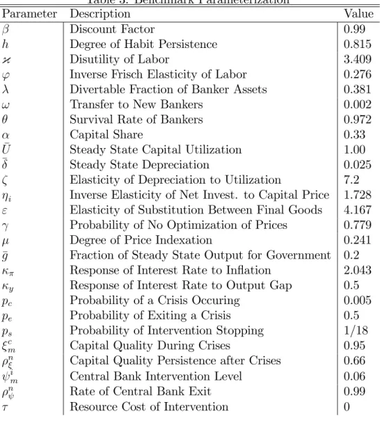
Figure 2 depicts the responses to the typical crisis with pi = 0 and pi = 1. When a crisis occurs, capital quality drops …ve percent for the duration of the crisis –two periods in this case –and then returns to its pre-crisis levels. When

pi = 0, the level of intervention remains at zero. The shock to capital quality reduces banker net worth, driving the leverage ratio up, and causing a drop in the price of capital, which creates a …nancial accelerator e¤ect of further diminishing the banker net worth. Since the …nancial intermediaries have less net worth, they are unable to borrow funds, driving interest rates down and spreads up, and capital declines with less investment. The increase in spreads lasts two quarters before declining, roughly corresponding to the recent crisis in the US, and in contrast to the one-period spike in spreads generated by a one-period shock. In total, the drop in output exceeds 10% from its pre-crisis level.

Whenpi = 1, the crisis is met by a jump in the level of intervention, which continues for 20 quarters beyond the initial crisis. The additional demand

for capital provided by the central bank in this circumstance works against the …nancial accelerator e¤ect: the price of capital drops slightly less, leading banker net worth to drop slightly less, and the leverage ratio and interest rate spreads to increase less than without intervention. The increased ability of the private sector to provide capital, as well as that provided by the central bank, yields a trough in output that is less than 9% of its pre-crisis levels. So intervention lessens the recession by about 2 percentage points. At t = 20, the central bank begins to unwind, and does so very gradually, since n = 0:99

in this case, leading to a smooth, albeit slow, transition of the economy back to its pre-crisis levels.

4.2

Exit Strategies

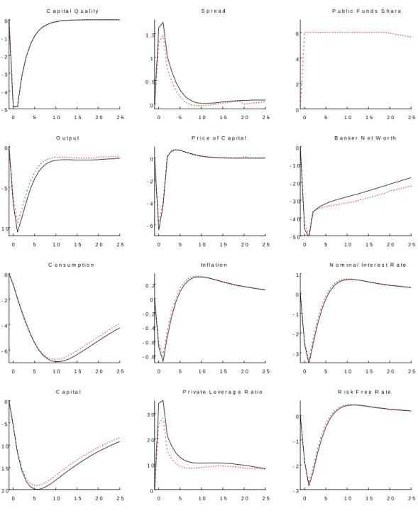
Suppose now that intervention is guaranteed(pi = 1), but that the unwind rate after intervention ends di¤ers. When the unwind rate is slow n _{= 0:99 , the} results comparing intervention versus no intervention showed that the economy transitions slowly but smoothly back to its pre-crisis level. Figure 3 shows the e¤ects of this slow unwind contrasted with the case of a sell-o¤ n _{= 0 . With} a sell-o¤, the intervention response is identical to the slow unwind case for the intervention period, but at t = 20, when the economy switches back to the "normal times" regime, the central bank immediately unloads its asset holdings rather then unwinding them over an extended period. There are two main implications of this sell-o¤: contemporaneous to the sell-o¤ and beforehand through expectations.

When the sell-o¤ occurs at t = 20, the central bank unloading its assets immediately is e¤ectively a …re sale of assets, which depresses the price of capital. The decline in the price of capital diminishes the net worth of bankers, leading to a decline in interest rates, and a jump in the private leverage ratio and the interest rate spread. Since the central bank no longer provides capital and the loss in net worth decreases the private sector’s ability to do so, the rebound in capital slows from a loss in investment, and output drops again, approximately two percentage points. Importantly, all of these responses

are similar to what occurred during the initial crisis, except that at t = 20

capital quality has fully recovered. In other words, the sell-o¤ creates a second …nancial crisis and there is a double-dip recession due exclusively to policy.

The second e¤ect of the policy di¤erence is through expectations. The slow unwind and sell-o¤ policies are identical during the intervention regimes, they only di¤er once unwind begins. However, expectations of the sell-o¤ versus the slow unwind matter during this period when policies are identical. When agents in the economy expect a sell-o¤ to occur at some future date, they must worry about the crisis but also the double-dip recession. In fact, given household consumption smoothing through habits, they have a stronger incentive to provide more labor and save to smooth consumption through the ensuing double dip. As a consequence, the intial loss in capital when the sell-o¤ is expected is not as dramatic as when the slow unwind is expected, banker net worth is lower, and the private leverage ratio is higher and spreads lower during the intervening period. The initial drop in output from the crisis is also slightly less, implying that, with the sell-o¤ policy, the initial downturn is less severe, but the economy experiences a double-dip recession when the central bank unloads its assets.

4.3

Holding Duration

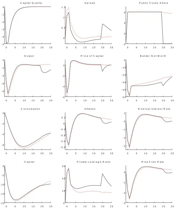
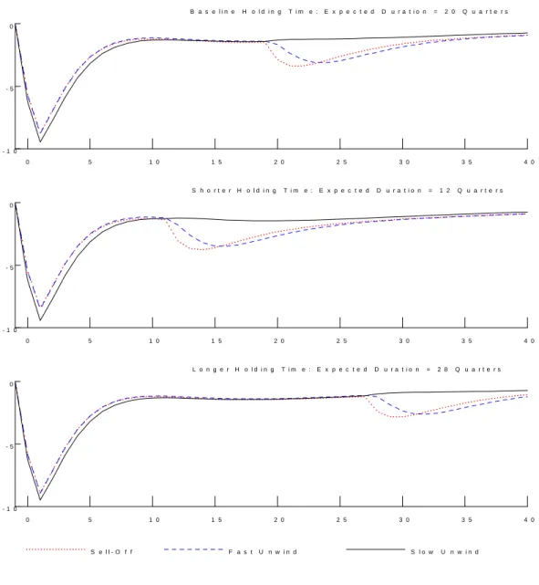
Having discussed the fact that an exit strategy of an immediate sell-o¤ pro-duces slightly better a slightly better outcome through the expectations chan-nel but creates a double-dip recession when the sell-o¤ occurs, it is important to consider the holding duration as well as the possibility for a sell-o¤ that is neither immediate but not very slow. Figure 4 shows the responses of output to the baseline duration of20total quarters versus the alternatives of a shorter or longer holding time, at 12 or28 quarters, respectively. For each duration, the …gure shows the responses to both the slow unwind n = 0:99 and the sell o¤ n _{= 0 previously considered, but also a fast unwind} n _{= 0:5 .}

Changing the expected holding duration produces similar responses to the baseline duration, but with di¤erences in magnitude. For all durations, the

slow unwind produces a gradual recovery in output to its pre-crisis level, and the sell-o¤ produces an initial drop that is not quite as large but generates a double-dip recession when the central bank exits from its asset position. With a shorter holding duration, the di¤erence in the trough of output between the slow unwind and sell-o¤ is larger than for the baseline duration, re‡ecting the incentive for households to smooth consumption from habits described in the previous subsection. The size of the double-dip recession decreases with duration: selling-o¤ assets soon after the crisis with a still-weak economy leads to larger negative e¤ects. The sell-o¤ after the longer holding duration still produces the double-dip recession, however.

In addition to the change in duration, the fast unwind case is a mixture between the slow unwind and the sell-o¤ cases. With the fast unwind, the central bank exits quickly, but not immediately. The result, for all three expected durations, is a double-dip that is less immediate but has the same size of trough. Consequently, selling o¤ assets quickly does still produce a double-dip recession, but a more gradual one that simply delays the recovery.

5

Pre-Crisis: E¤ects of Expectations

The previous section focused on the e¤ects of intervention and exit strategies during crises, this section examines the e¤ects of expectations of intervention and exit strategies during non-crisis times. The Markov switching framework established in Section 3 gives agents expectations that crises can occur, as well as expectations about the probability of intervention by the central bank, and the duration of intervention and exit strategy if intervention does occur. These expectations a¤ect prices and quantities before crises occur. Consequently, this section examines how the stochastic steady state of the economy associated with the "normal times" regime changes as the probability of intervention conditional on a crisis increases frompi = 0 to pi = 1, and the implications of the expected exit strategy.

Foersteret al. (2011) show that, in general, economies with Markov switch-ing that a¤ects the steady state of the economy are not certainty equivalent,

which implies that the stochastic steady state associated with each regime de-pends upon probability distributions across future regimes. In addition, the perturbation method allows a second-order approximation to the solution, and this higher-order expansion can provide more accurate descriptions of how the stochastic steady state for each regime varies. An alternative explanation of the "normal times" regime-conditional stochastic steady state is that it is the average over a long simulation of the economy, where agents expect that crises can occur and have certain expectations about intervention probabilities and exits, but ex-post in the simulation no crises occur.

5.1

Changes in Pre-Crisis Stochastic Steady State

In the baseline parameterization, agents perceive the probability of crises to be pc = 0:005, the exit probability to be pe = 0:5, and the probability of stopping intervention to beps = 1=18. Figure 5 shows the percent change in the "normal times" stochastic steady state relative to a benchmark economy where pc = 0, meaning agents do not expect crises, and hence expectations about intervention policy are irrelevant.

Consider the baseline parameterization with pc = 0:005 but pi = 0, so intervention policy is irrelevant and hence the slow unwind and sell-o¤ cases are identical. Moving from an economy where agents do not expect crises

(pc= 0), to one where they expect crises without intervention has two main implications. Households, on the one hand, have an incentive to precautionary save in order to smooth consumption during times of crises. In the stochastic steady state, this incentive increases household savings, boosting up capital accumulation and raising output and consumption. On the other hand, crises bring poor interest rate realizations for bankers, who will supply more net worth, have lower leverage, and consequently create a lower amount of capital for the economy, leading to lower output and consumption. In the aggregate, the latter of these e¤ects dominates: the economy with crises has 0.75% lower capital, 0.445% lower output, and 0.285% lower consumption than would be realized in an economy that never experienced crises.

Now, as pi increases from 0 to 1, agents expect intervention with a higher probability. Since intervention dampens the e¤ects of crises, increasing the probability of intervention erodes household’s precautionary incentive, lower-ing capital and output, but raises capital and output by favorable interest rate conditions for bankers. In aggregate, as pi increases, consumption declines, but capital and output increase if the sell-o¤ exit strategy is used, but decline if the slow unwind is in place. Consumption also declines more for the slow unwind case than the sell-o¤, which, since a sell-o¤ produces a double-dip recession, gives more incentive for households to save and boost consumption.

5.2

Expectations and Habits

To highlight the impact of the opposing channels, households’precautionary savings versus bankers’interest rates, and the e¤ects of expectations of policy, Figure 6 contrasts the change in the "normal times" stochastic steady state that prevails under the baseline calibration with habits (h = 0:815) with that of no habits (h= 0). In the no habits case, the households have signi…cantly lower incentive to precautionary save, since their smoothing motive is dimin-ished. As a result, the no habits case has capital, output, and consumption signi…cantly lower, as the lack of precautionary motive lessens the buildup of household savings. As the probability of intervention pi increases, the main e¤ect is to improve the expected spread, which, in equilibrium, leads to lower leverage and higher banker net worth.

6

Welfare Calculations

Having considered the e¤ects of policy announcements and expectations during and before crises, this section turns to evaluating the overall welfare gains or losses from di¤erent policy announcements. In particular, Section 4 discussed the fact that guaranteed intervention had bene…ts relative to no intervention during crises, since intervention helps bolster the economy and alleviate the crisis. However, there was a slight trade-o¤ depending upon the exit strategy:

the immediate sell-o¤ case produced a slightly lower drop in output and con-sumption, but upon exit, the economy experienced a double-dip recession. In addition, in Section 5, the e¤ects of increasing the probability of intervention had negative e¤ects on pre-crisis consumption. Since crises are rare events, whether or not the continual loss in consumption caused by increasing the chance of intervention outweighs the bene…ts of intervention during the crises is ultimately a welfare question.

Importantly, in addition to the probability of intervention and the exit strategy considered, welfare costs will be a¤ected by two factors. First, the resource cost of central bank intermediation will matter for welfare in that, if the cost is high, then a larger portion of output is lost, which may lower welfare. Second, the timing of the calculation matters for welfare costs. Speci…cally, the household’s gain or loss in welfare from di¤erent policies will depend upon whether they are experiencing a crisis or not. In other words, the ex-ante

welfare costs measure the willingness to pay for intervention before a crisis, while theex-post welfare costs measure willingness to pay when a crisis occurs. Forex-ante andex-post welfare, the welfare measure used is the percentage increase in expected lifetime consumption under guaranteed no intervention that would make households indi¤erent between the increase in consumption and an policy of a given probability of intervention and exit strategy. Positive welfare measures indicate that intervention is welfare-increasing, since house-holds need additional consumption under the given speci…cation to mimic pos-itive intervention probabilities. Negative welfare measures then imply inter-vention is welfare-decreasing, as households are willing to give up consumption rather than have positive intervention probabilities.

A second-order expansion to the value function formulation of household preferences (1) allows for accurate welfare measures that incorporate both the e¤ects of crises and the e¤ects of expectations in generating di¤erences in the "normal times" stochastic steady state.

6.1

Welfare and the Resource Cost

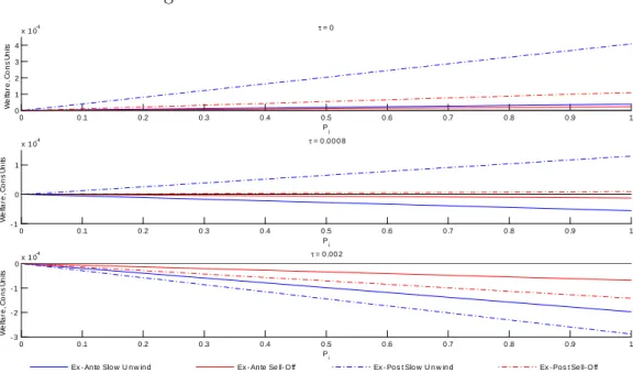
Figure 7 depicts the change in the welfare measure as the resource cost and the intervention probabilitypi change. The top panel shows the baseline case, when = 0, which corresponds to no e¢ ciency loss from intermediation, the second and third panels show = :0008 and = :002, respectively. Each panel shows the welfare measure in consumption units for a given intervention probability, both with the slow unwind n _{=:99 and the fast sell-o¤} n _{= 0} cases. In addition, they compare welfare when the economy is in the "normal times" regime versus when the economy has experienced a crisis but before realization of the intervention outcome.

The …rst panel shows that, when = 0, increases in intervention proba-bility are welfare improving in both the crisis and pre-crisis scenarios. Since there is no resource cost of intervention, and given the magnitude of drops in output and consumption relative to the change in pre-crisis consumption, hav-ing intervention is welfare improvhav-ing. It is interesthav-ing to note that the slow unwind exit strategy dominates the fast sell-o¤ strategy in both ex-ante and

ex-post circumstances. Since the slow unwind tended to smooth output after crises, this fact implies that agents place emphasis on avoiding the double-dip recession that the sell-o¤ can produce. In addition, conditional on an exit strategy, the bene…t from having positive intervention probability is higher once a crisis occurs.

The second and third panels change the implications of intervention. In the second panel, when = :0008, the results about the type of intervention and timing change. For both types of exit strategy, the welfare bene…ts of increasing the intervention probability are negative when the economy is in the "normal times" regime, and positive when the economy enters a crisis. This case suggests that there may be a type of time-inconsistency in the opti-mal intervention policy. Before a crisis, it households prefer no intervention because of the distortions caused by this guarantee and the resource cost of in-tervention, but when a crisis occurs, increasing the probability of intervention is welfare improving. Further, conditional upon intervention, the welfare-preferred exit strategy changes from preferring a sell-o¤ex-ante to preferring

a slow unwindex-post.

The third panel has = :002, when the welfare bene…ts are negative for all the cases, meaning increasing the probability of intervention is welfare decreasing. This fact holds true regardless of the exit strategy used and the timing. Further, theex-post welfare losses are higher, and the losses are higher when the exit strategy is to unwind assets slowly. Both of these results stem from the relatively high resource cost of intervention: when intervention is costly in terms of output, there is a welfare loss from intervention, especially when a crisis occurs –because intervention is immediate –and welfare losses are higher when the intervention takes longer to unwind.

The di¤erent levels of the resource cost dictate which policy environment is best from a welfare perspective. Importantly, under the = 0:0008 pa-rameterization for both types of crises, the better rule in terms of welfare changed ex-ante versus ex-post. Prior to a crisis occurring, positive inter-vention probabilities are welfare decreasing, and the better rule is the fast unwind, but when a crisis occurs positive probabilities are welfare increasing, and the welfare preferred rule is the slow unwind. These changes between the ex-ante versus ex-post welfare implications suggest that there may be a time-inconsistency in optimal policy and hence commitment may be di¢ cult.

6.2

Welfare and Holding Duration

Figure 7 shows that the di¤erences between the ex-ante and ex-post welfare measures when = 0:0008 are fairly robust to holding duration. The …gure uses = 0:0008, and now the probability of stopping varies from ps = 1=18 to the shorter holding duration ps = 1=10 and the longer durationps = 1=26 considered in the crises responses of Figure 4. As noted previously, when the expected duration is20 quarters, then increasing the intervention probability increases welfare ex-post, and the dominate exit strategy is the slow unwind; whereas increase the probability decreases welfare ex-ante and the dominant exit strategy is the sell-o¤.

hardly change. When the duration is shorter, at12quarters, the main di¤er-ence is the negativity of theex-post sell-o¤ welfare measure. In this case, even when a crisis is occurring, the economy is better o¤ with no intervention than with intervention, because the intervention period is so short and is followed by a sell-o¤ of assets that creates a double-dip recession. In other words, agents would rather the central bank not intervene than intervene but exit rapidly and after a short period.

7

Conclusion

This paper used a model of unconventional monetary policy along with regime switching to study the e¤ects of exit strategies and agents pre-crisis expecta-tions. After intervention, if the central bank exits its unconventional policy with a sell-o¤, the economy experiences a double-dip recession. In addition, increasing the probability of intervention during crises causes distortions in pre-crisis activity by altering agents’expectations; in particular, pre-crisis sto-chastic steady state consumption falls as the intervention probability increases. Finally, the welfare bene…ts of increasing the probability of intervention can raise or lower welfare, and that the timing of the welfare calculation matters as well as the type of exit strategy used.

One interesting avenue for future research is make the probability and magnitude of intervention endogenous and dependent on the extent of the crisis. This paper assumed …xed crisis magnitudes, levels of intervention, and probabilities. Larger crises presumably have a higher probability and levels of intervention. In addition, the probability of crises is …xed and exogenous; moral hazard could be captured in the model by having a state-dependent probability of crisis. Since expectations about future intervention probabilities and exit strategies a¤ect the pre-crisis state, policy declarations could serve to increase or decrease the probability of crises. Similarly, the probability the central bank starts to unwind its balance sheet may depend upon how quickly the economy rebounds after the crisis. Finally, this paper has focused on a given class of policy, optimal policy within this class is left for future work.

References

Angeloni, I., Faia, E., & Winkler, R.2011. Exit Strategies.Kiel Institute Working Paper.

Barro, R.2006. Rare Disasters and Asset Markets in the Twentieth Century.

Quarterly Journal of Economics, 121(3), 823–866.

Barro, R.2009. Rare Disasters, Asset Prices, and Welfare Costs. American Economic Review,99(1), 243–264.

Barro, R., Nakamura, E., Steinsson, J., & Ursua, J. 2010. Crises and Recoveries in an Empirical Model of Consumption Disasters. NBER Working Paper, 15920.

Bernanke, B., & Gertler, M.1989. Agency Costs, Net Worth, and Busi-ness Fluctuations. American Economic Review, 79(1), 14–31.

Bernanke, B., Gertler, M., & Gilchrist, S. 1999. The Financial Acel-erator in a Quantitative Business Cycle Framework. Handbook of Macroeco-nomics, 1, 1341–1393.

Bianchi, F.2010. Regime Switches, Agents’Beliefs, and Post-World War II US Macroeconomic Dynamics. Working Paper.

Bianchi, J.2011. Overborrowing and Systemic Externalities in the Business Cycle. American Economic Review,101(7), 3400–3426.

Brunnermeier, M., & Sannikov, Y.2011. A Macroeconomic Model with a Financial Sector. Working Paper.

Carlstrom, C.and Fuerst, T.1997. Agency Costs, Net Worth, and Busi-ness Fluctuations: A Computable General Equilibrium Analysis. American Economic Review,87(5), 893–910.

Chari, VV, & Kehoe, P. 2009. Bailouts, Time Inconsistency and Optimal Regulation. Federal Reserve Bank of Minneapolis Sta¤ Report.

Christiano, L., Eichenbaum, M., & Evans, C. 2005. Nominal Rigidities and the Dynamic E¤ects of a Shock to Monetary Policy.Journal of Political Economy, 113(1), 1–45.

Christiano, L., Motto, R., & Rostagno, M. 2010. Financial Factors in Economic Fluctuations. ECB Working Paper, 1192.

Cúrdia, V., & Woodford, M. 2010a. Conventional and Unconventional Monetary Policy. Federal Reserve Bank of St. Louis Review,92(4), 229–264.

Cúrdia, V., & Woodford, M.2010b. Credit Spreads and Monetary Policy.

Journal of Money, Credit and Banking, 42(S1), 3–35.

Cúrdia, V., & Woodford, M. 2011. The Central Bank Balance Sheet as an Instrument of Monetary Policy. Journal of Monetary Economics, 58(1), 54–79.

Davig, T., & Leeper, E.2007. Generalizing the Taylor Principle. American Economic Review,97(3), 607–635.

Del Negro, M., Eggertsson, G., Ferrero, A., & Kiyotaki, N. 2010. The Great Escape? A Quantitative Evaluation of the Fed’s Non-Standard Policies. Federal Reserve Bank of New York Sta¤ Report,520.

Farmer, R, Waggoner, D., & Zha, T. 2008. Minimal State Variable Solutions to Markov-Switching Rational Expectations Models. Journal of Economic Dynamics and Control,35(12), 2150–2166.

Farmer, R, Waggoner, D., & Zha, T. 2009. Understanding Markov-Switching Rational Expectations Models. Journal of Economic Theory,

144(5), 1849–1867.

Foerster, A., Rubio-Ramirez, J., Waggoner, D., & Zha, T. 2011. Perturbation Methods for Markov Switching Models. Mimeo.

Gertler, M., & Karadi, P. 2010. A Model of Unconventional Monetary Policy. Journal of Monetary Economics, 58(1), 17–34.

Gertler, M., & Kiyotaki, N. 2010. Financial Intermediation and Credit Policy in Business Cycle Analysis. Handbook of Monetary Economics, 3, 547–599.

Gertler, M., Kiyotaki, N., & Queralto, A. 2010. Financial Crises, Bank Risk Exposure and Government Financial Policy. Working Paper.

Gourio, F. 2010. Disasters Risk and Business Cycles. American Economic Review, Forthcoming.

Hilberg, B., & Hollmayr, J. 2011. Asset Prices, Collateral and Uncon-ventional Monetary Policy in a DSGE Model. ECB Working Paper, 1373.

Kiyotaki, N., & Moore, J. 1997. Credit Cycles. Journal of Political Economy, 105(2), 211–248.

Kiyotaki, N., & Moore, J.2008. Liquidity, Business Cycles, and Monetary Policy. Working Paper.

Merton, R.C. 1973. An Intertemporal Capital Asset Pricing Model. Econo-metrica,41(5), 867–887.

Perri, F., & Quadrini, V.2011. International Recessions. NBER Working Paper, 17201.

Primiceri, G., Schaumburg, E., & Tambalotti, A.2006. Intertemporal Disturbances. NBER Working Paper, 12243.

Rietz, T.1988. The Equity Risk Premium: A Solution. Journal of Monetary Economics, 22(1), 117–131.

Shleifer, A., & Vishny, R.W. 2010. Asset Fire Sales and Credit Easing.

American Economic Review,100(2), 46–50.

Smets, R., & Wouters, F. 2007. Shocks and Frictions in US Business Cycles: a Bayesian DSGE Approach. American Economic Review, 97(3), 586–606.

Figure 1: Federal Reserve’s Balance Sheet 20050 2006 2007 2008 2009 2010 2011 0.5 1 1.5 2 2.5 3 B a la n ce S he et ($ T ri l) D ate 2005 2006 2007 2008 2009 2010 2011 1 2 3 4 5 6 7 S p re a d ( % P o in ts )

Balanc e Sheet (left) N on-Tr eas ur y As s ets (left) BAA - 10Year Treas ury ( r ight)

Table 1: Markov Switching Parameters

st m(st) (st) m(st) (st)

1) "Normal" 1 n ₀ n

2) "Crisis without Intervention" c_m 0 0 n 3) "Crisis with Intervention" cm 0

i

m 0

4) "Post-Crisis with Intervention" 1 n i_m 0

Table 2: Markov Switching Probabilities

st+1 1 2 3 4 1 1 pc pc(1 pi) pcpi 0 st 2 pe 1 pe 0 0 3 peps 0 1 pe pe(1 ps) 4 (1 pc)ps 0 pc (1 pc) (1 ps)

Table 3: Benchmark Parameterization

Parameter Description Value

Discount Factor 0.99

h Degree of Habit Persistence 0.815

{ Disutility of Labor 3.409

' Inverse Frisch Elasticity of Labor 0.276

Divertable Fraction of Banker Assets 0.381

! Transfer to New Bankers 0.002

Survival Rate of Bankers 0.972

Capital Share 0.33

U Steady State Capital Utilization 1.00

Steady State Depreciation 0.025

Elasticity of Depreciation to Utilization 7.2 i Inverse Elasticity of Net Invest. to Capital Price 1.728

" Elasticity of Substitution Between Final Goods 4.167 Probability of No Optimization of Prices 0.779

Degree of Price Indexation 0.241

g Fraction of Steady State Output for Government 0.2 Response of Interest Rate to In‡ation 2.043 y Response of Interest Rate to Output Gap 0.5

pc Probability of a Crisis Occuring 0.005

pe Probability of Exiting a Crisis 0.5

ps Probability of Intervention Stopping 1/18 c

m Capital Quality During Crises 0.95

n _{Capital Quality Persistence after Crises 0.66} i

m Central Bank Intervention Level 0.06

n _{Rate of Central Bank Exit 0.99}

Figure 2: Responses Under a Guarantee 0 5 1 0 1 5 2 0 2 5 - 5 - 4 - 3 - 2 - 1 0 C a p i t a l Q u a l i t y 0 5 1 0 1 5 2 0 2 5 0 0 . 5 1 1 . 5 S p r e a d 0 5 1 0 1 5 2 0 2 5 0 2 4 6 P u b l i c F u n d s S h a r e 0 5 1 0 1 5 2 0 2 5 - 1 0 - 5 0 O u t p u t 0 5 1 0 1 5 2 0 2 5 - 6 - 4 - 2 0 P r i c e o f C a p i t a l 0 5 1 0 1 5 2 0 2 5 - 5 0 - 4 0 - 3 0 - 2 0 - 1 0 0 B a n k e r N e t W o r t h 0 5 1 0 1 5 2 0 2 5 - 6 - 4 - 2 0 C o n s u m p t i o n 0 5 1 0 1 5 2 0 2 5 - 0 . 8 - 0 . 6 - 0 . 4 - 0 . 2 0 0 . 2 I n f l a t i o n 0 5 1 0 1 5 2 0 2 5 - 3 - 2 - 1 0 1 N o m i n a l I n t e r e s t R a t e 0 5 1 0 1 5 2 0 2 5 - 2 0 - 1 5 - 1 0 - 5 0 C a p i t a l 0 5 1 0 1 5 2 0 2 5 0 1 0 2 0 3 0 P r i v a t e L e v e r a g e R a t i o 0 5 1 0 1 5 2 0 2 5 - 3 - 2 - 1 0 R i s k F r e e R a t e I n t e r v e n e N o I n t e r v e n e

Figure 3: Exit Strategies: Slow Unwind versus Sell-O¤ 0 5 1 0 1 5 2 0 2 5 - 5 - 4 - 3 - 2 - 1 0 C a p i t a l Q u a l i t y 0 5 1 0 1 5 2 0 2 5 0 0 . 5 1 1 . 5 S p r e a d 0 5 1 0 1 5 2 0 2 5 0 2 4 6 P u b l i c F u n d s S h a r e 0 5 1 0 1 5 2 0 2 5 - 8 - 6 - 4 - 2 0 O u t p u t 0 5 1 0 1 5 2 0 2 5 - 6 - 4 - 2 0 P r i c e o f C a p i t a l 0 5 1 0 1 5 2 0 2 5 - 5 0 - 4 0 - 3 0 - 2 0 - 1 0 0 B a n k e r N e t W o r t h 0 5 1 0 1 5 2 0 2 5 - 6 - 4 - 2 0 C o n s u m p t i o n 0 5 1 0 1 5 2 0 2 5 - 0 . 8 - 0 . 6 - 0 . 4 - 0 . 2 0 0 . 2 I n f l a t i o n 0 5 1 0 1 5 2 0 2 5 - 3 - 2 - 1 0 1 N o m i n a l I n t e r e s t R a t e 0 5 1 0 1 5 2 0 2 5 - 2 0 - 1 5 - 1 0 - 5 0 C a p i t a l 0 5 1 0 1 5 2 0 2 5 0 1 0 2 0 3 0 P r i v a t e L e v e r a g e R a t i o 0 5 1 0 1 5 2 0 2 5 - 3 - 2 - 1 0 R i s k F r e e R a t e S l o w U n w i n d S e l l - O f f

Figure 4: Output Responses to Holding Durations and Exit Strategies 0 5 1 0 1 5 2 0 2 5 3 0 3 5 4 0 - 1 0 - 5 0 B a s e l i n e H o l d i n g T i m e : E x p e c t e d D u r a t i o n = 2 0 Q u a r t e r s 0 5 1 0 1 5 2 0 2 5 3 0 3 5 4 0 - 1 0 - 5 0 S h o r t e r H o l d i n g T i m e : E x p e c t e d D u r a t i o n = 1 2 Q u a r t e r s 0 5 1 0 1 5 2 0 2 5 3 0 3 5 4 0 - 1 0 - 5 0 L o n g e r H o l d i n g T i m e : E x p e c t e d D u r a t i o n = 2 8 Q u a r t e r s S e l l - O f f F a s t U n w i n d S l o w U n w i n d

Figure 5: E¤ects of Expectations 0 0.2 0.4 0.6 0.8 1 -0.31 -0.3 -0.29 -0.28 P i % C han ge Consumption 0 0.2 0.4 0.6 0.8 1 0.014 0.016 0.018 0.02 P i % C han ge Inflation 0 0.2 0.4 0.6 0.8 1 -0.85 -0.8 -0.75 -0.7 -0.65 P i % C han ge Capital 0 0.2 0.4 0.6 0.8 1 0.02 0.025 0.03 0.035 0.04 P_i % C han ge Price of Capital 0 0.2 0.4 0.6 0.8 1 -3.5 -3 -2.5 P_i % C han ge

Private Leverage Ratio

0 0.2 0.4 0.6 0.8 1 1.5 2 2.5 3 P_i % C han ge Net Worth 0 0.2 0.4 0.6 0.8 1 -0.46 -0.45 -0.44 -0.43 P i % C han ge Output 0 0.2 0.4 0.6 0.8 1 -20 -18 -16 -14 P i % C han ge Expected Spread 0 0.2 0.4 0.6 0.8 1 0.01 0.015 0.02 P i % C han ge Nominal Rate

Slow Unwind Sell-Off

Figure 6: E¤ects of Expectations and Impact of Habits

0 0.2 0.4 0.6 0.8 1 -4 -3 -2 -1 0 P_i % C ha nge Consumption 0 0.2 0.4 0.6 0.8 1 0.014 0.016 0.018 0.02 P_i % C ha nge Inflation 0 0.2 0.4 0.6 0.8 1 -6 -4 -2 0 P_i % C ha nge Capital 0 0.2 0.4 0.6 0.8 1 0.02 0.025 0.03 0.035 0.04 P_i % C ha nge Price of Capital 0 0.2 0.4 0.6 0.8 1 -4 -3.5 -3 -2.5 P_i % C ha nge

Private Leverage Ratio

0 0.2 0.4 0.6 0.8 1 -2 0 2 4 P_i % C ha nge Net Worth 0 0.2 0.4 0.6 0.8 1 -4 -3 -2 -1 0 P_i % C ha nge Output 0 0.2 0.4 0.6 0.8 1 -20 -18 -16 -14 P_i % C ha nge Expected Spread 0 0.2 0.4 0.6 0.8 1 0.01 0.015 0.02 P_i % C ha nge Nominal Rate

Figure 7: Welfare and the Resource Cost 0 0 .1 0 .2 0 .3 0 .4 0 .5 0 .6 0 .7 0 .8 0 .9 1 0 1 2 3 4 x 1 0-4 P_i W e lfar e, C ons U ni ts τ = 0 0 0 .1 0 .2 0 .3 0 .4 0 .5 0 .6 0 .7 0 .8 0 .9 1 - 1 0 1 x 1 0-4 P_i W e lfar e, C ons U ni ts τ = 0 .0 0 0 8 0 0 .1 0 .2 0 .3 0 .4 0 .5 0 .6 0 .7 0 .8 0 .9 1 - 3 - 2 - 1 0x 1 0 -4 P i W e lfar e, C ons U ni ts τ = 0 .0 0 2 Ex - An te Slo w U n w in d Ex - An te Se ll- O ff Ex - Po s t Slo w U n w in d Ex - Po s t Se ll- O ff

Figure 8: Welfare and Holding Duration

0 0 .1 0 .2 0 .3 0 .4 0 .5 0 .6 0 .7 0 .8 0 .9 1 - 1 0 1 2 3x 1 0 -4 P_i We lfa re , C o n s Un its Ex p e c te d D u r a tio n = 2 0 0 0 .1 0 .2 0 .3 0 .4 0 .5 0 .6 0 .7 0 .8 0 .9 1 - 5 0 5 1 0 1 5x 1 0 -5 P i We lfa re , C o n s Un its Ex p e c te d D u r a tio n = 1 2 0 0 .1 0 .2 0 .3 0 .4 0 .5 0 .6 0 .7 0 .8 0 .9 1 - 1 0 1 2 3x 1 0 -4 P_i We lfa re , C o n s Un its Ex p e c te d D u r a tio n = 2 8 Ex - An te Slo w U n w in d Ex - An te Se ll- O ff Ex - Po s t Slo w U n w in d Ex - Po s t Se ll- O ff