Searching the Web
Arvind Arasu Junghoo Cho Hector Garcia-Molina Andreas Paepcke Sriram Raghavan Computer Science Department, Stanford University
{arvinda,cho,hector,paepcke,rsram}@cs.stanford.edu Abstract
We offer an overview of current Web search engine design. After introducing a generic search engine architecture, we examine each engine component in turn. We cover crawling, local Web page storage, indexing, and the use of link analysis for boosting search performance. The most common design and implementation techniques for each of these components are presented. We draw for this presentation from the literature, and from our own experimental search engine testbed. Emphasis is on introducing the fundamental concepts, and the results of several performance analyses we conducted to compare different designs.
Keywords: Search engine, crawling, indexing, link analysis, PageRank, HITS, hubs, authorities, infor-mation retrieval.
1
Introduction
The plentiful content of the World-Wide Web is useful to millions. Some simply browse the Web
through entry points such as Yahoo!. But many information seekers use asearch engineto begin their
Web activity. In this case, users submit a query, typically a list of keywords, and receive a list of Web pages that may be relevant, typically pages that contain the keywords. In this paper we discuss the challenges in building good search engines, and describe some of the techniques that are useful.
Many of the search engines use well-known information retrieval (IR) algorithms and techniques [55, 28]. However, IR algorithms were developed for relatively small and coherent collections such as news-paper articles or book catalogs in a (physical) library. The Web, on the other hand, is massive, much less coherent, changes more rapidly, and is spread over geographically distributed computers. This requires new techniques, or extensions to the old ones, to deal with the gathering of the information, to make index structures scalable and efficiently updateable, and to improve the discriminating ability of search engines. For the last item, discriminating ability, it is possible to exploit the linkage among Web pages to better identify the truly relevant pages.
There is no question that the Web is huge and challenging to deal with. Several studies have estimated the size of the Web [4, 42, 41, 6], and while they report slightly different numbers, most of
them agree that over a billion pages are available. Given that the average size of a Web page is around 5–10K bytes, just the textual data amounts to at least tens of terabytes. The growth rate of the Web is even more dramatic. According to [41, 42], the size of the Web has doubled in less than two years, and this growth rate is projected to continue for the next two years.
Aside from these newly created pages, the existing pages are continuously updated [52, 58, 24, 17]. For example, in our own study of over half a million pages over 4 months [17], we found that about 23%
of pages changed daily. In the .comdomain 40% of the pages changed daily, and the half-life of pages
is about 10 days (in 10 days half of the pages are gone, i.e., their URLs are no longer valid). In [17], we also report that a Poisson process is a good model for Web page changes. Later in Section 2, we will show how some of these results can be used to improve search engine quality.
In addition to size and rapid change, the interlinked nature of the Web sets it apart from many other collections. Several studies aim to understand how the Web’s linkage is structured and how that structure can be modeled [11, 5, 2, 36, 17]. One recent study, for example, suggests that the link structure of the Web is somewhat like a “bow-tie” [11]. That is, about 28% of the pages constitute a strongly connected core (the center of the bow tie). About 22% form one of the tie’s loops: these are pages that can be reached from the core but not vice versa. The other loop consists of 22% of the pages that can reach the core, but cannot be reached from it. (The remaining nodes can neither reach the core nor can be reached from the core.)
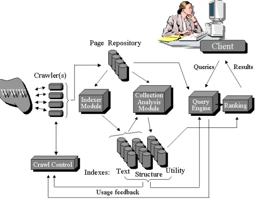
Figure 1: General search engine architecture
typically put together. Figure 1 shows such an engine schematically. Every engine relies on a crawler
module to provide the grist for its operation (shown on the left in Figure 1). Crawlers are small programs that ‘browse’ the Web on the search engine’s behalf, similarly to how a human user would follow links to reach different pages. The programs are given a starting set of URLs, whose pages they retrieve from the Web. The crawlers extract URLs appearing in the retrieved pages, and give this information to the
crawler control module. This module determines what links to visit next, and feeds the links to visit back to the crawlers. (Some of the functionality of the crawler control module may be implemented by
the crawlers themselves.) The crawlers also pass the retrieved pages into a page repository. Crawlers
continue visiting the Web, until local resources, such as storage, are exhausted.
This basic algorithm is modified in many variations that give search engines different levels of coverage or topic bias. For example, crawlers in one engine might be biased to visit as many sites as possible, leaving out the pages that are buried deeply within each site. The crawlers in other engines might specialize on sites in one specific domain, such as governmental pages. The crawl control module is responsible for directing the crawling operation.
Once the search engine has been through at least one complete crawling cycle, the crawl control module may be informed by several indexes that were created during the earlier crawl(s). The crawl
control module may, for example, use a previous crawl’s link graph (the structure index in Figure 1)
to decide which links the crawlers should explore, and which links they should ignore. Crawl control may also use feedback from usage patterns to guide the crawling process (connection between the query engine and the crawl control module in Figure 1). Section 2 will examine crawling operations in more detail.
The indexer module extracts all the words from each page, and records the URL where each word occurred. The result is a generally very large “lookup table” that can provide all the URLs that point to
pages where a given word occurs (thetext index in Figure 1). The table is of course limited to the pages
that were covered in the crawling process. As mentioned earlier, text indexing of the Web poses special difficulties, due to its size, and its rapid rate of change. In addition to these quantitative challenges, the Web calls for some special, less common kinds of indexes. For example, the indexing module may also create a structure index, which reflects the links between pages. Such indexes would not be appropriate
for traditional text collections that do not contain links. The collection analysis module is responsible
for creating a variety of other indexes.
The utility index in Figure 1 is created by the collection analysis module. For example, utility indexes may provide access to pages of a given length, pages of a certain “importance,” or pages with some number of images in them. The collection analysis module may use the text and structure indexes when creating utility indexes. Section 4 will examine indexing in more detail.
During a crawling and indexing run, search engines must store the pages they retrieve from the Web. The page repository in Figure 1 represents this—possibly temporary—collection. Sometimes search engines maintain a cache of the pages they have visited beyond the time required to build the
index. This cache allows them to serve out result pages very quickly, in addition to providing basic search facilities. Some systems, such as the Internet Archive [37], have aimed to maintain a very large number of pages for permanent archival purposes. Storage at such a scale again requires special consideration. Section 3 will examine these storage-related issues.
The query engine module is responsible for receiving and filling search requests from users. The engine relies heavily on the indexes, and sometimes on the page repository. Because of the Web’s size, and the fact that users typically only enter one or two keywords, result sets are usually very large. The ranking module therefore has the task of sorting the results such that results near the top are the most likely ones to be what the user is looking for. The query module is of special interest, because traditional information retrieval (IR) techniques have run into selectivity problems when applied without modification to Web searching: Most traditional techniques rely on measuring the similarity of query texts with texts in a collection’s documents. The tiny queries over vast collections that are typical for Web search engines prevent such similarity based approaches from filtering sufficient numbers of irrelevant pages out of search results. Section 5 will introduce search algorithms that take advantage of the Web’s interlinked nature. When deployed in conjunction with the traditional IR techniques, these algorithms significantly improve retrieval precision in Web search scenarios.
In the rest of this article we will describe in more detail the search engine components we have presented. We will also illustrate some of the specific challenges that arise in each case, and some of the techniques that have been developed. Our paper is not intended to provide a complete survey of techniques. As a matter of fact, the examples we will use to illustrate will be drawn mainly from our own work since it is what we know best.
In addition to research at universities and open laboratories, many “dot-com” companies have worked on search engines. Unfortunately, many of the techniques used by dot-coms, and especially the resulting performance, are kept private behind company walls, or are ‘disclosed’ in patents whose
language only lawyers can comprehend and appreciate. We therefore believe that the overview of
problems and techniques we provide here can be of use.
2
Crawling Web pages
The crawler module (Figure 1) retrieves pages from the Web for later analysis by the indexing module.
As discussed in the introduction, a crawler module typically starts off with an initial set of URLs S0.
Roughly, it first places S0 in a queue, where all URLs to be retrieved are kept and prioritized. From
this queue, the crawler gets a URL (in some order), downloads the page, extracts any URLs in the downloaded page, and puts the new URLs in the queue. This process is repeated until the crawler decides to stop. Given the enormous size and the change rate of the Web, many issues arise, including the following:
1. What pages should the crawler download? In most cases, the crawler cannot download all
pages on the Web. Even the most comprehensive search engine currently indexes a small fraction of the entire Web [42, 6]. Given this fact, it is important for the crawler to carefully select the pages and to visit “important” pages first by prioritizing the URLs in the queue properly, so that the fraction of the Web that is visited (and kept up-to-date) is more meaningful.
2. How should the crawler refresh pages? Once the crawler has downloaded a significant
number of pages, it has to start revisiting the downloaded pages in order to detect changes and
refresh the downloaded collection. Because Web pages are changing at very different rates [18, 58], the crawler needs to carefully decide what page to revisit and what page to skip, because this decision may significantly impact the “freshness” of the downloaded collection. For example, if a certain page rarely changes, the crawler may want to revisit the page less often, in order to visit more frequently changing ones.
3. How should the load on the visited Web sites be minimized? When the crawler collects pages from the Web, it consumes resources belonging to other organizations [39]. For example, when the crawler downloads pagepon siteS, the site needs to retrieve pagepfrom its file system, consuming disk and CPU resource. Also, after this retrieval the page needs to be transferred through the network, which is another resource shared by multiple organizations. The crawler should minimize its impact on these resources [54]. Otherwise, the administrators of the Web site or a particular network may complain and sometimes completely block access by the crawler. 4. How should the crawling process be parallelized? Due to the enormous size of the Web,
crawlers often run on multiple machines and download pages in parallel [10, 18]. This paralleliza-tion is often necessary in order to download a large number of pages in a reasonable amount of time. Clearly these parallel crawlers should be coordinated properly, so that different crawlers do not visit the same Web site multiple times, and the adopted crawling policy should be strictly enforced. The coordination can incur significant communication overhead, limiting the number of simultaneous crawlers.
In the rest of this section we discuss the first two issues, page selection and page refresh, in more detail. We do not discuss load or parallelization issues, mainly because much less research has been done on those topics.
2.1 Page selection
As we argued, the crawler may want to download “important” pages first, so that the downloaded collection is of high quality. There are three questions that need to be addressed: the meaning of “importance,” how a crawler operates, and how a crawler “guesses” good pages to visit. We discuss these questions in turn, using our own work to illustrate some of the possible techniques.
2.1.1 Importance metrics
Given a Web page P, we can define the importance of the page in one of the following ways: (These
metrics can be combined, as will be discussed later.)
1. Interest Driven. The goal is to obtain pages “of interest” to a particular user or set of users. So important pages are those that match the interest of users. One particular way to define this
notion is through what we call a driving query. Given a query Q, the importance of page P is
defined to be the “textual similarity” [55] between P and Q. More formally, we compute textual
similarity by first viewing each document (P orQ) as an m-dimensional vectorhw1, . . . , wni. The
term wi in this vector represents the ith word in the vocabulary. If wi does not appear in the
document, thenwi is zero. If it does appear, wi is set to represent the significance of the word.
One common way to compute the significancewi is to multiply the number of times theith word
appears in the document by the inverse document frequency (idf) of theith word. Theidf factor
is one divided by the number of times the word appears in the entire “collection,” which in this
case would be the entire Web. Then we define thesimilaritybetweenP andQas acosine product
between the P and Q vectors [55]. Assuming that query Q represents the user’s interest, this
metric shows how “relevant”P is. We use IS(P) to refer to this particular importance metric.
Note that if we do not use idf terms in our similarity computation, the importance of a page,
IS(P), can be computed with “local” information, i.e.,P andQ. However, if we useidfterms, then we need global information. During the crawling process we have not seen the entire collection, so
we have to estimate theidffactors from the pages that have been crawled, or from some reference
idf terms computed at some other time. We use IS0(P) to refer to the estimated importance of
pageP, which is different from the actual importance IS(P), which can be computed only after
the entire Web has been crawled.
Reference [16] presents another interest-driven approach based on a hierarchy of topics. Interest is defined by a topic, and the crawler tries to guess the topic of pages that will be crawled (by analyzing the link structure that leads to the candidate pages).
2. Popularity Driven. Page importance depends on how “popular” a page is. For instance, one way
to define popularity is to use a page’s backlink count. (We use the term backlink for links that
point to a given page.) Thus a Web page P’s backlinks are the set of all links on pages other
thanP, which point toP. When using backlinks as a popularity metric, the importance value of
P is the number of links to P that appear over the entire Web. We use IB(P) to refer to this
importance metric. Intuitively, a pageP that is linked to by many pages is more important than
one that is seldom referenced. This type of “citation count” has been used in bibliometrics to
evaluate the impact of published papers. On the Web, IB(P) is useful for ranking query results,
requires counting backlinks over the entire Web. A crawler may estimate this value withIB0(P),
the number of links toP that have been seen so far. (The estimate may be inaccurate early on in
a crawl.) Later in Section 5 we define a similar yet more sophisticated metric, called PageRank
IR(P), that can also be used as a popularity measure.
3. Location Driven. TheIL(P) importance of pageP is a function of its location, not of its contents.
If URLu leads toP, then IL(P) is a function ofu. For example, URLs ending with “.com” may
be deemed more useful than URLs with other endings, or URLs containing the string “home” may be of more interest than other URLs. Another location metric that is sometimes used considers URLs with fewer slashes more useful than those with more slashes. Location driven metrics can be considered a special case of interest driven ones, but we list them separately because they are often easy to evaluate. In particular, all the location metrics we have mentioned here are local
since they can be evaluated simply by looking at the URLu.
As stated earlier, our importance metrics can be combined in various ways. For example, we may define a metric IC(P) =k1·IS(P) +k2·IB(P) +k3·IL(P), for some constants k1,k2,k3 and query
Q. This combines the similarity metric, the backlink metric and the location metric.
2.1.2 Crawler models
Our goal is to design a crawler that if possible visits high importance pages before lower ranked ones,
for a certain importance metric. Of course, the crawler will only haveestimatedimportance values (e.g.,
IB0(P)) available. Based on these estimates, the crawler will have to guess the high importance pages
to fetch next. For example, we may define the quality metric of a crawler in one of the following two
ways:
• Crawl & Stop: Under this model, the crawler C starts at its initial page P0 and stops after
visiting K pages. (K is a fixed number determined by the number of pages that the crawler can
download in one crawl.) At this point a perfect crawler would have visited pages R1, . . . , RK,
where R1 is the page with the highest importance value, R2 is the next highest, and so on. We
call pages R1 through RK the hot pages. The K pages visited by our real crawler will contain
only M (≤ K) pages with rank higher than or equal to that of RK. (Note that we need to
know the exact rank of all pages in order to obtain the value M. Clearly, this estimation may
not be possible until we download all pages and obtain the global image of the Web. Later in Section 2.1.4, we restrict the entire Web to the pages in the Stanford domain and estimate the
ranks of pages based on this assumption.) Then we define the performance of the crawler C to
be PCS(C) = (M ·100)/K. The performance of the ideal crawler is of course 100%. A crawler
that somehow manages to visit pages entirely at random, and may revisit pages, would have a
is a hot page with probabilityK/T. Thus, the expected number of desired pages when the crawler stops isK2/T.)
• Crawl & Stop with Threshold: We again assume that the crawler visitsK pages. However, we
are now given an importance targetG, and any page with importance higher thanGis considered
hot. Let us assume that the total number of hot pages isH. Again, we assume that we know the
ranks of all pages and thus can to obtain the value H. The performance of the crawler, PST(C),
is the percentage of the H hot pages that have been visited when the crawler stops. IfK < H ,
then an ideal crawler will have performance (K·100)/H. If K ≥H, then the ideal crawler has
100% performance. A purely random crawler that revisits pages is expected to visit (H/T)·K
hot pages when it stops. Thus, its performance is (K·100)/T. Only if the random crawler visits
all T pages, is its performance expected to be 100%.
2.1.3 Ordering metrics
A crawler keeps a queue of URLs it has seen during the crawl, and must select from this queue the next
URL to visit. The ordering metric is used by the crawler for this selection, i.e., it selects the URL u
such that theordering valueof uis the highest among all URLs in the queue. The ordering metric can
only use information seen (and remembered if space is limited) by the crawler.
The ordering metric should be designed with an importance metric in mind. For instance, if we are
searching for high IB(P) pages, it makes sense to use an IB0(P) as the ordering metric, where P is
the page upoints to. However, it might also make sense to consider an IR0(P) (the PageRank metric,
Section 5), even if our importance metric is the simpler citation count. In the next subsection we show why this may be the case.
Location metrics can be used directly for ordering, since the URL of P directly gives the IL(P)
value. However, for similarity metrics, it is much harder to devise an ordering metric, since we have not
seen P yet. We may be able to use the text that anchors the URL u as a predictor of the text that P
might contain. Thus, one possible ordering metric isIS(A) (for some query Q), whereA is the anchor
text of the URL u. Reference [23] proposes an approach like this, where not just the anchor text, but
all the text of a page (and “near” pages) is considered forIS(P).
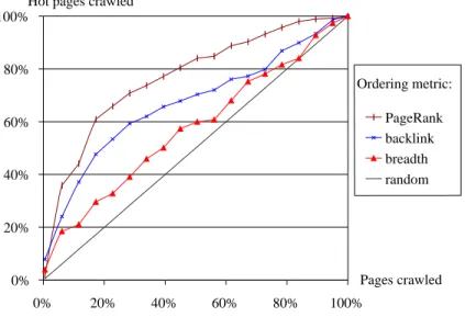
2.1.4 Case Study
To illustrate that it is possible to download important pages significantly earlier when we adopt an appropriate ordering metric, we show some results from an experiment we conducted. To keep our experiment manageable, we defined the entire Web to be the 225,000 Stanford University Web pages that were downloaded by our Stanford WebBase crawler. That is, we assumed that all pages outside Stanford have “zero importance value,” and that links to pages outside Stanford or from pages outside
Stanford do not count in page importance computations. Note that since the pages were downloaded by our crawler, they are all reachable from the Stanford homepage.
Under this assumption, we experimentally measured the performance of various ordering metrics
for the importance metric IB(P), and we show the result in Figure 2. In this graph, we assumed the
Crawl & Stop model with Threshold, with threshold value G = 100. That is, pages with more than
100 backlinks were considered “hot,” and we measured how many hot pages were downloaded when the
crawler had visitedx% of the Stanford pages. Under this definition, the total number of hot pages was
1,400, which was about 0.8% of all Stanford pages. The horizontal axis represents the percentage of
pages downloaded from the Stanford domain, and the vertical axis shows the percentage of hot pages
downloaded.
In the experiment, the crawler started at the Stanford homepage (http://www.stanford.edu) and,
in three different experimental conditions, selected the next page visit either by the ordering metric
IR0(P) (PageRank), by IB0(P) (backlink), or by following links breadth-first (breadth). The straight line in the graph shows the expected performance of a random crawler.
0% 20% 40% 60% 80% 100% 0% 20% 40% 60% 80% 100% PageRank backlink breadth random Ordering metric: Pages crawled Hot pages crawled
Figure 2: The performance of various ordering metrics forIB(P); G= 100
From the graph, we can clearly see that an appropriate ordering metric can significantly improve
the performance of the crawler. For example, when the crawler used IB0(P) (backlink) as its ordering
metric, the crawler downloaded more than 50% of hot pages, when it visited less than 20% of the entire Web. This is a significant improvement compared to a random crawler or a breadth first crawler, which downloaded less than 30% of hot pages at the same point. One interesting result of this experiment
is that the PageRank ordering metric, IR0(R), shows better performance than the backlink ordering
metric IB0(R), even when the importance metric is IB(R). This is because of the inheritance property of the PageRank metric, which can help avoid downloading “locally popular” pages before “globally popular,” but “locally unpopular” pages. In additional experiments [20] (not described here) we study
other metrics, and also observe that the right ordering metric can significantly improve the crawler performance.
2.2 Page refresh
Once the crawler has selected and downloaded “important” pages, it has to periodically refresh the downloaded pages, so that the pages are maintained up-to-date. Clearly there exist multiple ways to update the pages, and different strategies will result in different “freshness” of the pages. For example, consider the following two strategies:
1. Uniform refresh policy: The crawler revisits all pages at the same frequency f, regardless of how often they change.
2. Proportional refresh policy: The crawler revisits a page proportionally more often, as it changes more often. More precisely, assume thatλi is the change frequency of a pageei, and that
fi is the crawler’s revisit frequency for ei. Then the frequency ratio λi/fi is the same for any i. For example, if pagee1 changes 10 times more often than pagee2, the crawler revisitse1 10 times more often thane2.
Note that the crawler needs to estimate λi’s for each page, in order to implement this policy.
This estimation can be based on the change history of a page that the crawler can collect [17].
For example, if a crawler visited/downloaded a page p1 every day for a month, and it detected
10 changes, the crawler may reasonable estimate that λ1 is one change every 3 days. For more
detailed discussion onλestimation, see [17].
Between these two strategies, which one will give us higher “freshness?” Also, can we come up with an even better strategy? To answer these questions, we need to understand how Web pages change over time and what we mean by “freshness” of pages. In the next two subsections, we go over possible answers to these questions and compare various refresh strategies.
2.2.1 Freshness metric
Intuitively, we consider a collection of pages “fresher” when the collection has more up-to-date pages.
For instance, consider two collections,AandB, containing the same 20 web pages. Then ifAmaintains
10 pages up-to-date on average, and ifB has maintains 15 up-to-date pages, we considerB to be fresher
thanA. Also, we have a notion of “age:” even if all pages are obsolete, we consider collection A “more
current” than B, if Awas refreshed 1 day ago, and B was refreshed 1 year ago. Based on this intuitive
notion, we have found the following definitions of freshnessandage to be useful. (Incidentally, [21] has a slightly different definition of freshness, but it leads to results that are analogous to ours.) In the
following discussion, we refer to the pages on the Web that the crawler monitors as thereal-world pages
1. Freshness: LetS ={e1, . . . , eN}be the local collection ofN pages. Then we define thefreshness of the collection as follows.
Definition 1 The freshnessof a local pageei at timetis
F(ei;t) = (
1 ifei is up-to-date at time t
0 otherwise.
(By up-to-date we mean that the content of a local page equals that of its real-world counterpart.) Then, thefreshness of the local collection S at timet is
F(S;t) = 1 N N X i=1 F(ei;t).
The freshness is the fraction of the local collection that is up-to-date. For instance, F(S;t) will be one if all local pages are up-to-date, andF(S;t) will be zero if all local pages are out-of-date.
2. Age: To capture “how old” the collection is, we define the metricage as follows:
Definition 2 The age of the local pageei at timetis
A(ei;t) = (
0 ifei is up-to-date at time t
t−modification time of ei otherwise. Then theage of the local collection S is
A(S;t) = 1 N N X i=1 A(ei;t).
Theageof S tells us the average “age” of the local collection. For instance, if all real-world pages changed one day ago and we have not refreshed them since,A(S;t) is one day.
Obviously, the freshness (and age) of the local collection may change over time. For instance, the freshness might be 0.3 at one point of time, and it might be 0.6 at another point of time. Because of this possible fluctuation, we now compute the average freshness over a long period of time and use this value as the “representative” freshness of a collection.
Definition 3 We define the time average of freshness of pageei, ¯F(ei), and the time average of freshness of collection S, ¯F(S), as ¯ F(ei) = limt→∞ 1 t Z t 0 F(ei;t)dt ¯ F(S) = lim t→∞ 1 t Z t 0 F(S;t)dt.
The time average of age can be defined similarly. 2
Mathematically, the time average of freshness or age may not exist, because we take a limit over time. However, the above definition approximates the fact that we take the average of freshness over a long
period of time. Later on, we will see that the time averagedoesexist when pages change by a reasonable
2.2.2 Refresh strategy
In comparing the page refresh strategies, it is important to note that crawlers can download/update only a limited number of pages within a certain period, because crawlers have limited resources. For example, many search engines report that their crawlers typically download several hundred pages per second. (Our own crawler, which we call the WebBase crawler, typically runs at the rate of 50–100
pages per second.) Depending on the page refresh strategy, this limitedpage download resource will be
allocated to different pages in different ways. For example, the proportional refresh policy will allocate this download resource proportionally to the page change rate.
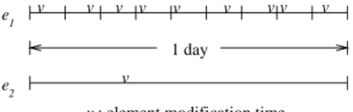
To illustrate the issues, consider a very simple example. Suppose that the crawler maintains a
collection of two pages: e1 and e2. Page e1 changes 9 times per day and e2 changes once a day. Our
goal is to maximize the freshness of the database averaged over time. In Figure 3, we illustrate our simple model. For page e1, one day is split into 9 intervals, and e1 changes once and only oncein each
interval. However, we do not know exactly when the page changes within an interval. Page e2 changes
once and only onceper day, but we do not know precisely when it changes.
1 day
e2 v
: element modification time
v
e1 v v v v v v vv v
Figure 3: A database with two pages with different change frequencies
Because our crawler is a tiny one, assume that we can refresh one page per day. Then what page
should it refresh? Should the crawler refreshe1or should it refreshe2? To answer this question, we need to compare how the freshness changes if we pick one page over the other. If pagee2changes in the middle of the day and if we refreshe2 right after the change, it will remain up-to-date for the remaining half of the day. Therefore, by refreshing pagee2 we get 1/2 day “benefit”(or freshness increase). However, the probability thate2 changes before the middle of the day is 1/2, so the “expected benefit” of refreshing
e2 is 1/2×1/2 day = 1/4 day. By the same reasoning, if we refresh e1 in the middle of an interval,
e1 will remain up-to-date for the remaining half of the interval (1/18 of the day) with probability 1/2. Therefore, the expected benefit is 1/2×1/18 day = 1/36 day. From this crude estimation, we can see that it is more effective to select e2 for refresh!
Of course, in practice, we do not know for sure that pages will change in a given interval.
Further-more, we may also want to worry about the age of data. (In our example, if we always visite2, the age
of e1 will grow indefinitely.)
In [19], we have studied a more realistic scenario, using the Poisson process model. In particular, we
can mathematically prove that the uniform policy is always superior or equal to the proportional one,
metrics, when page changes follow Poisson processes. For a detailed proof, see [19].
In [19] we also show how to obtain the optimal refresh policy (better than uniform or any other), assuming page changes follow a Poisson process and their change frequencies are static (i.e., do not
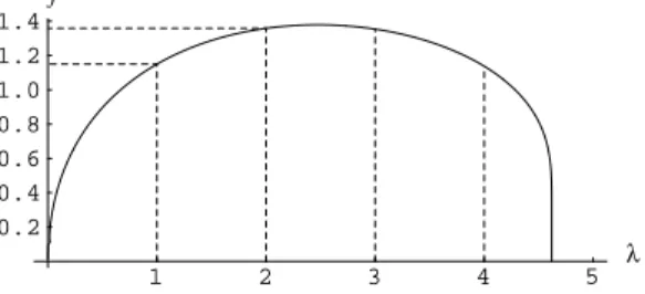
change over time). To illustrate, in Figure 4 we show the refresh frequencies that maximizes the
freshness value for a simple scenario. In this scenario, the crawler maintains 5 pages with change
rates, 1,2, . . . ,5 (times/day), respectively, and the crawler can download 5 pages per day. The graph in Figure 4 shows the needed refresh frequency of a page (vertical axis) as a function of its change frequency (horizontal axis), in order to maximize the freshness of the 5 page collection. For instance,
the optimal revisit frequency for the page that changes once a day is 1.15 times/day. Notice that the
graph does not monotonically increase over change frequency, and thus we need to refresh pages less
often if the pages change too often. The pages with change frequency larger than 2.5 times/day should
be refreshed less often than the ones with change frequency 2 times/day. When a certain page changes too often, and if we cannot maintain it up-to-date under our resource constraint, it is in fact better to focus our resource on the pages that we can keep track of.
1 2 3 4 5 λ 0.2 0.4 0.6 0.8 1.0 1.2 1.4 f
Figure 4: change frequency vs. refresh frequency for freshness optimization
Figure 4 is for a particular 5-page scenario, but in [19] we prove that the shape of the graph is the
same forany distribution of change frequencies under the Poisson process model. That is, the optimal
graph forany collection of pagesS isexactly the sameas Figure 4, except that the graph ofS is scaled
by a constant factor from Figure 4. Thus, no matter what the scenario, pages that change too frequently (relative to the available resources) should be penalized and not visited very frequently.
We can obtain the optimal refresh policy for the age metric, as described in [19].
2.3 Conclusion
In this section, we discussed the challenges that a crawler encounters when it downloads large collections
of pages from the Web. In particular, we studied how a crawler shouldselectandrefresh the pages that
it retrieves and maintains.
There are, of course, still many open issues. For example, it is not clear how a crawler and a Web site can negotiate/agree on a right crawling policy, so that the crawler does not interfere with the primary operation of the site, while downloading the pages on the site. Also, existing work on crawler
parallelization is either ad hoc or quite preliminary, so we believe this issue needs to be carefully studied. Finally, some of the information on the Web is now “hidden” behind a search interface, where a query must be submitted or a form filled out. Current crawlers cannot generate queries or fill out forms, so they cannot visit the “dynamic” content. This problem will get worse over time, as more and more sites generate their Web pages from databases.
3
Storage
Thepage repository in Figure 1 is a scalable storage system for managing large collections of Web pages. As shown in the figure, the repository needs to perform two basic functions. First, it must provide an interface for the crawler to store pages. Second, it must provide an efficient access API that the indexer and collection analysis modules can use to retrieve the pages. In the rest of the section, we present some key issues and techniques for such a repository.
3.1 Challenges
A repository manages a large collection of “data objects”, namely, Web pages. In that sense, it is conceptually quite similar to other systems that store and manage data objects (e.g., file systems and database systems). However, a Web repository does not have to provide a lot of the functionality that the other systems provide (e.g., transactions, logging, directory structure) and instead, can be targeted to address the following key challenges:
Scalability: It must be possible to seamlessly distribute the repository across a cluster of computers and disks, in order to cope with the size of the Web (see Section 1).
Dual access modes: The repository must support two different access modes equally efficiently.
Random access is used to quickly retrieve a specific Web page, given the page’s unique identifier.
Streaming access is used to receive the entire collection, or some significant subset, as a stream of pages. Random access is used by the query engine to serve out cached copies to the end-user. Streaming access is used by the indexer and analysis modules to process and analyze pages in bulk.
Large bulk updates: Since the Web changes rapidly (see Section 1), the repository needs to handle a high rate of modifications. As new versions of Web pages are received from the crawler, the space
occupied by old versions must be reclaimed1 through space compaction and reorganization. In addition,
excessive conflicts between the update process and the applications accessing pages must be avoided. 1Some repositories might maintain a temporal history of Web pages by storing multiple versions for each page. We do
Obsolete pages: In most file or data systems, objects are explicitly deleted when no longer needed. However, when a Web page is removed from a Web site, the repository is not notified. Thus, the repository must have a mechanism for detecting and removing obsolete pages.
3.2 Designing a distributed Web repository
Let us consider a generic Web repository that is designed to function over a cluster of interconnected
storage nodes. There are three key issues that affect the characteristics and performance of such a repository:
• Page distribution across nodes
• Physical page organization within a node
• Update strategy
3.2.1 Page distribution policies
Pages can be assigned to nodes using a number of different policies. For example, with a uniform
distribution policy, all nodes are treated identically. A given page can be assigned to any of the nodes in the system, independent of it’s identifier. Nodes will store portions of the collection proportionate to their storage capacities. In contrast, with ahash distribution policy, allocation of pages to nodes would depend on the page identifiers. In this case, a page identifier would be hashed to yield a node identifier and the page would be allocated to the corresponding node. Various other policies are also possible. Reference [35] contains qualitative and quantitative comparisons of the uniform and hash distribution policies in the context of a Web repository.
3.2.2 Physical page organization methods
Within a single node, there are three possible operations that could be executed: page addition/insertion,
high-speed streaming, and random page access. Physical page organization at each node is a key factor that determines how well a node supports each of these operations.
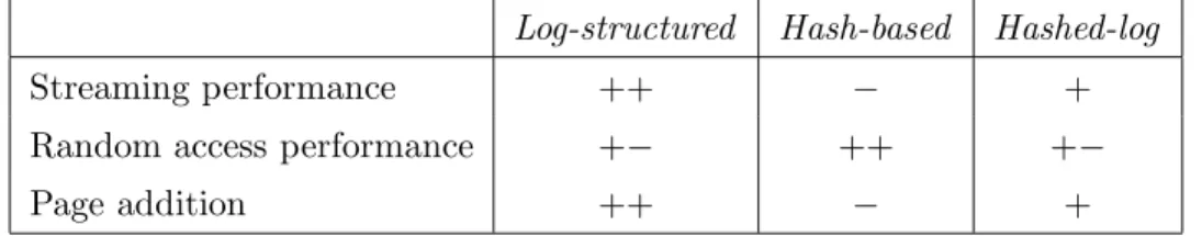
There are several options for page organization. For example, a hash-based organization treats a disk (or disks) as a set of hash buckets, each of which is small enough to fit in memory. Pages are assigned to hash buckets depending on their page identifier. Since page additions are common, a log-structured organization may also be advantageous. In this case, the entire disk is treated as a large contiguous log to which incoming pages are appended. Random access is supported using a separate B-tree index that maps page identifiers to physical locations on disk. One can also devise a hybrid hashed-log organization, where storage is divided into large sequential “extents,” as opposed to buckets that fit in memory. Pages are hashed into extents, and each extent is organized like a log-structured
file. In [35] we compare these strategies in detail, and Table 1 summarizes the relative performance. Overall, a log-based scheme works very well, except if many random-access requests are expected.
Log-structured Hash-based Hashed-log
Streaming performance ++ − +
Random access performance +− ++ +−
Page addition ++ − +
Table 1: Comparing page organization methods
3.2.3 Update strategies
Since updates are generated by the crawler, the design of the update strategy for a Web repository depends on the characteristics of the crawler. In particular, there are at least two ways in which a crawler may be structured:
Batch-mode or Steady crawler: A batch-mode crawler is periodically executed, say once every month, and allowed to crawl for a certain amount of time (or until a targeted set of pages have been crawled) and then stopped. With such a crawler, the repository receives updates only for a certain number of days every month. In contrast, a steady crawler runs without any pause, continuously supplying updates and new pages to the repository.
Partial or Complete crawls: A batch-mode crawler may be configured to either perform a complete crawl every time it is run, or recrawl only a specific set of pages or sites. In the first case, pages from the new crawl completely replace the old collection of pages already existing in the repository. In the second case, the new collection is created by applying the updates of the partial crawl to the existing collection. Note that this distinction between partial and complete crawls does not make sense for steady crawlers. Depending on these two factors, the repository can choose to implement either in-place update or shadowing. With in-place updates, pages received from the crawler are directly integrated into the repository’s existing collection, possibly replacing older versions. With shadowing, pages from a crawl are stored separate from the existing collection and updates are applied in a separate step. As shown in
Figure 5, theread nodes contain the existing collection and are used to service all random and streaming
access requests. The update nodes store the set of pages retrieved during the latest crawl.
The most attractive characteristic of shadowing is the complete separation between updates and read accesses. A single storage node does not ever have to concurrently handle page addition and page retrieval. This avoids conflicts, leading to improved performance and a simpler implementation. On the downside, since there is a delay between the time a page is retrieved by the crawler and the time the page is available for access, shadowing may decrease collection freshness.
In our experience, a batch-mode crawler generating complete crawls matches well with a shadowing repository. Analogously, a steady crawler can be better matched with a repository that uses in-place updates. Furthermore, shadowing has a greater negative impact on freshness with a steady crawler than with a batch-mode crawler. For additional details, see [18].
LA N C raw ler Indexer A nalyst Read nodes Update nodes Node manager
Figure 5: WebBase repository architecture
3.3 The Stanford WebBase repository
To illustrate how all the repository factors fit in, we briefly describe the Stanford WebBase repository, and the choices that were made. The WebBase repository is a distributed storage system that works in conjunction with the Stanford WebCrawler. The repository operates over a cluster of storage nodes
connected by a high-speed communication network (see Figure 5). The repository employs a node
manager to monitor the individual storage nodes and collect status information (such as free space, load, fragmentation, and number of outstanding access requests). The node manager uses this information to control the operations of the repository and schedule update and access requests on each node.
Each page in the repository is assigned a unique identifier, derived by computing a signature (e.g., checksum or cyclic redundancy check) of the URL associated with the page. However, a given
URL can have multiple text string representations. For example, http://WWW.STANFORD.EDU:80/and
http://www.stanford.edurepresent the same Web page but would give rise to different signatures. To
avoid this problem, the URL is first normalized to yield a canonical representation [35]. The identifier
is computed as a signature of this normalized URL.
Since the Stanford WebCrawler is a batch-mode crawler, the WebBase repository employs the shad-owing technique. It can be configured to use different page organization methods and distribution policies on the read nodes and update nodes. Hence, the update nodes can be tuned for optimal page addition performance and the read nodes, for optimal read performance.
3.4 Conclusion
The page repository is an important component of the overall Web search architecture. It must efficiently support the different access patterns of the query engine (random access) and the indexer modules (streaming access). It must also employ an update strategy that is tuned to the characteristics of the crawler.
In this section, we focused on the basic functionality required of a Web repository. However, there are a number of other features that might be useful for specific applications. Below, we suggest possible enhancements:
Multiple media types: So far, we have assumed that Web repositories store only plain text or HTML pages. However, with the growth of non-text content on the Web, it is becoming increasingly important to store, index, and search over image, audio, and video collections.
Advanced streaming: In our discussion of streaming access, we have assumed that the streaming order was not important. This is sufficient for building most basic indexes including the text and structure indexes of Figure 1. However, for more complicated indexes, the ability to retrieve a specific subset (e.g., pages in the “.edu” domain) and/or in a specified order (e.g., in increasing order by citation rank) may be useful.
4
Indexing
The indexer and collection analysis modules in Figure 1 build a variety of indexes on the collected pages. The indexer module builds two basic indexes: a text (or content) index and a structure (or
link index). Using these two indexes and the pages in the repository, the collection analysis module
builds a variety of other useful indexes. Below, we will present a short description of each type of index, concentrating on their structure and use.
Link index: To build a link index, the crawled portion of the Web is modeled as a graph with nodes
and edges. Each node in the graph is a Web page and a directed edge from nodeAto nodeB represents
a hypertext link in page A that points to page B. An index on the link structure must be a scalable
and efficient representation of this graph.
Often, the most common structural information used by search algorithms [8, 38] is neighborhood
information, i.e., given a pageP, retrieve the set of pages pointed to byP (outward links) or the set of
pages pointing toP (incoming links). Disk-based adjacency list representations [1] of the original Web
graph and of the inverted Web graph2 can efficiently provide access to such neighborhood information.
Other structural properties of the Web graph can be easily derived from the basic information stored in 2In the inverted Web graph, the direction of the hypertext links are reversed.
these adjacency lists. For example, the notion of sibling pages is often used as the basis for retrieving pages “related” to a given page (see Section 5). Such sibling information can be easily derived from the pair of adjacency list structures described above.
Small graphs of hundreds or even thousands of nodes can be efficiently represented by any one of a variety of well-known data structures [1]. However, doing the same for a graph with several million
nodes and edges is an engineering challenge. In [7], Bharath et. al. describe the Connectivity Server,
a system to scalably deliver linkage information for all pages retrieved and indexed by the Altavista search engine.
Text index: Even though link-based techniques are used to enhance the quality and relevance of search results, text-based retrieval (i.e., searching for pages containing some keywords) continues to be the primary method for identifying pages relevant to a query. Indexes to support such text-based retrieval can be implemented using any of the access methods traditionally used to search over text
document collections. Examples include suffix arrays [43], inverted files or inverted indexes [55, 59],
and signature files [27]. Inverted indexes have traditionally been the index structure of choice on the Web. We will discuss inverted indexes in detail later on in the section.
Utility indexes: The number and type of utility indexes built by the collection analysis module depends on the features of the query engine and the type of information used by the ranking mod-ule. For example, a query engine that allows searches to be restricted to a specific site or domain
(e.g., www.stanford.edu) would benefit from a site index that maps each domain name to a list of
pages belonging to that domain. Similarly, using neighborhood information from the link index, an iterative algorithm (see Section 5) can easily compute and store the PageRank [8] associated with each page in the repository. Such an index would be used at query time to aid in the ranking of search results.
For the rest of this section, we will focus our attention on text indexes. In particular, we will address the problem of quickly and efficiently building inverted indexes over Web-scale collections.
4.1 Structure of an inverted index
An inverted index over a collection of Web pages consists of a set of inverted lists, one for each word
(orindex term). The inverted list for a term is a sorted list oflocations where the term appears in the collection. In the simplest case, alocation will consist of a page identifier and the position of the term in the page. However, search algorithms often make use of additional information about the occurrence of terms in a Web page. For example, terms occurring in bold face (within<B>tags), in section headings (within <H1>or <H2>tags), or as anchor text might be weighted differently in the ranking algorithms.
encodes whatever additional information needs to be maintained about each term occurrence. Given an index term w, and a corresponding location l, we refer to the pair (w, l) as a posting forw.
In addition to the inverted lists, most text-indexes also maintain what is known as a lexicon. A
lexicon lists all the terms occurring in the index along with some term-level statistics (e.g., total number of documents in which a term occurs) that are used by the ranking algorithms [55, 59].
4.2 Challenges
Conceptually, building an inverted index involves processing each page to extract postings, sorting the postings first on index terms and then on locations, and finally writing out the sorted postings as a collection of inverted lists on disk. For relatively small and static collections, as in the environments traditionally targeted by information retrieval (IR) systems, index build times are not very critical. However, when dealing with Web-scale collections, naive index build schemes become unmanageable and require huge resources, often taking days to complete. As a measure of comparison with traditional IR systems, our 40 million page WebBase repository (Section 3.3) represents only about 4% of the
publicly indexable Web but is already larger than the 100 GB very large TREC-7 collection [34], the benchmark for large IR systems.
In addition, since content on the Web changes rapidly (see Section 1), periodic crawling and rebuild-ing of the index is necessary to maintain “freshness.” Index rebuilds become necessary because most incremental index update techniques perform poorly when confronted with the huge wholesale changes commonly observed between successive crawls of the Web [46].
Finally, storage formats for the inverted index must be carefully designed. A small compressed index improves query performance by allowing large portions of the index to be cached in memory. However, there is a tradeoff between this performance gain and the corresponding decompression overhead at query time [47, 49, 59]. Achieving the right balance becomes extremely challenging when dealing with Web-scale collections.
4.3 Index partitioning
Building a Web-scale inverted index requires a highly scalable and distributed text-indexing architecture. In such an environment, there are two basic strategies for partitioning the inverted index across a collection of nodes [44, 53, 56].
In the local inverted file (IFL) organization [53], each node is responsible for a disjoint subset of pages in the collection. A search query would be broadcast to all the nodes, each of which would return disjoint lists of page identifiers containing the search terms.
Global inverted file (IFG)organization [53] partitions on index terms so that each query server stores inverted lists only for a subset of the terms in the collection. For example, in a system with two query
ranges[a-q] whereasB could store the inverted lists for the remaining index terms. Therefore, a search
query that asks for pages containing the term “process”would only involve A.
Reference [45] describes certain important characteristics of the IFL strategy, such as resilience to node failures and reduced network load, that make this organization ideal for the Web search
environ-ment. Performance studies in [56] also indicate thatIFL organization uses system resources effectively
and provides good query throughput in most cases.
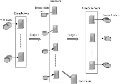
Figure 6: WebBase indexing architecture
4.4 WebBase Text-Indexing System
Our experience in building a text index for our WebBase repository serves to illustrate the problems faced in building a massive index. Indeed, our index was built to facilitate tests with different solutions, so we were able to obtain experimental results that show some of the tradeoffs. In the rest of this subsection we provide an overview of the WebBase index and the techniques utilized.
4.4.1 System overview
Our indexing system operates on a shared-nothing architecture consisting of a collection of nodes
con-nected by a local area network (Figure 6). We identify three types of nodes in the system.3 The
distributors are part of the WebBase repository (Section 3) and store the collection of Web pages to
be indexed. The indexers execute the core of the index building engine. The final inverted index is
partitioned across thequery servers using theIFL strategy discussed in Section 4.3.
The WebBase indexing system builds the inverted index in two stages. In the first stage, each
dis-tributor node runs adistributor process that disseminates the pages to the indexers using the streaming
access mode provided by the repository. Each indexer receives a mutually disjoint subset of pages and their associated identifiers. The indexers parse and extract postings from the pages, sort the postings
in memory, and flush them to intermediate structures (sorted runs) on disk.
In the second stage, these intermediate structures are merged together to create one or more inverted
files and their associated lexicons. An(inverted file, lexicon)pair is generated by merging a subset
of the sorted runs. Each pair is transferred to one or more query servers depending on the degree of index replication.
4.4.2 Parallelizing the index-builder
The core of our indexing engine is theindex-builder process that executes on each indexer. We
demon-strate below that this process can be effectively parallelized by structuring it as a software pipeline.
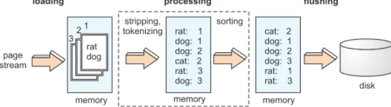
rat: 1 dog: 1 dog: 2 cat: 2 rat: 3 dog: 3 cat: 2 dog: 1 dog: 2 dog: 3 rat: 1 rat: 3 loading processing sorting stripping, tokenizing flushing page stream 1 2 3 rat dog disk
memory memory memory
Figure 7: Logical phases
The input to the index-builder is a sequence of Web pages and their associated identifiers. The
output of the index-builder is a set of sorted runs, each containing postings extracted from a subset
of the pages. The process of generating these sorted runs can logically be split into three phases as illustrated in Figure 7. We refer to these phases asloading,processing, andflushing. During the loading phase, some number of pages are read from the input stream and stored in memory. The processing phase involves two steps. First, the pages are parsed, tokenized into individual terms, and stored as a set of postings in a memory buffer. In the second step, the postings are sorted in-place, first by term, and then by location. During the flushing phase, the sorted postings in the memory buffer are saved on disk as a sorted run. These three phases are executed repeatedly until the entire input stream of pages has been consumed.
Loading, processing and flushing tend to use disjoint sets of system resources. Processing is obviously CPU-intensive, whereas flushing primarily exerts secondary storage, and loading can be done directly from the network or a separate disk. Therefore, indexing performance can be improved by executing these three phases concurrently (see Figure 8). Since the execution order of loading, processing and flushing is fixed, these three phases together form asoftware pipeline.
thread 1 thread 2 thread 3 indexing time 0 L P F L P F L P F L P F L P F L P F period:
3 * p optimal useof resources good use of resources wasted resources F: flushing P: processing L: loading
Figure 8: Multi-threaded execution of index-builder
phases that will result in minimal overall running time. Our problem differs from a typicaljob scheduling
problem [12] in that we can vary the sizes of the incomingjobs, i.e., in every loading phase we can choose the number of pages to load.
Consider an index-builder that uses N executions of the pipeline to process the entire collection of
pages and generate N sorted runs. By an execution of the pipeline, we refer to the sequence of three
phases — loading, processing, and flushing — that transform some set of pages into a sorted run. Let
Bi, i= 1. . . N, be the buffer sizes used during theseN executions. The sum
PN
i=1Bi =Btotal is fixed for a given amount of input and represents the total size of all the postings extracted from the pages.
In [45], we show that for an indexer with a single resource of each type (single CPU, single disk, and a single network connection over which to receive the pages), optimal speedup of the pipeline is achieved when the buffer sizes are identical in all executions of the pipeline, i.e., B =B1. . . =BN = BtotalN . In addition, we show how bottleneck analysis can be used to derive an expression for the optimal value
of B in terms of various system parameters. In [45], we also extend the model to incorporate indexers
with multiple CPU’s and disks.
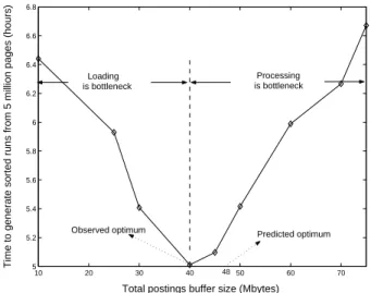
Experiments: We conducted a number of experiments using a single index-builder to verify our model and measure the effective performance gain achieved through a parallelized index-builder. Figure 9 highlights the importance of the theoretical analysis as an aid in choosing the right buffer size. Even though the predicted optimum size differs slightly from the observed optimum, the difference in running times between the two sizes is less than 15 minutes for a 5 million page collection. Figure 10 shows how pipelining impacts the time taken to process and generate sorted runs for a variety of input sizes. Note that for small collections of pages, the performance gain through pipelining, though noticeable, is not substantial. This is because small collections require very few pipeline executions and the overall time is dominated by the time required at startup (to load up the buffers) and shutdown (to flush the buffers). Our experiments showed that in general, for large collections, a sequential index-builder is
10 20 30 40 50 60 70 5 5.2 5.4 5.6 5.8 6 6.2 6.4 6.6 6.8
Total postings buffer size (Mbytes)
Time to generate sorted runs from 5 million pages (hours)
Predicted optimum 48 Observed optimum Loading is bottleneck Processing is bottleneck
Figure 9: Optimal buffer size
about 30–40% slower than a pipelined index-builder.
0 5 10 15 20 25 30 35 40 45 50 0 1 2 3 4 5 6 7
Number of pages indexed (in 100,000’s)
Time to generate sorted runs (in hours)
No pipelining (48MB total buffer size) Pipelining (48MB total buffer size)
Figure 10: Performance gain through pipelining
4.4.3 Efficient global statistics collection
As mentioned in Section 4, term-level4 statistics are often used to rank the search results of a query.
For example, one of the most commonly used statistic isinverse document frequency or IDF. The IDF
of a term w, is defined as logdfN
w, where N is the total number of pages in the collection and dfw is
the number of pages that contain at least one occurrence of w [55]. In a distributed indexing system,
when the indexes are built and stored on a collection of machines, gathering global (i.e., collection-wide) 4Term-level refers to the fact that any gathered statistic describes only single terms, and not higher level entities such
term-level statistics, with minimum overhead, becomes an important issue [57].
Some authors suggest computing global statistics at query time. This would require an extra round
of communication among the query servers to exchange local statistics5. However, this
communica-tion adversely impacts query processing performance, especially for large colleccommunica-tions spread over many servers.
Statistics-collection in WebBase: To avoid this query time overhead, the WebBase indexing system
precomputes and stores statistics as part of index creation. A dedicated server known as thestatistician
(see Figure 6) is used for computing statistics. Local information from the indexers is sent to the statistician as the pages are processed. The statistician computes the global statistics and broadcasts them back to all the indexers. These global statistics are then integrated into the lexicons during the merging phase, when the sorted runs are merged to create inverted files (see Section 4.4.1). Two techniques are used to minimize the overhead of statistics collection.
• Avoiding explicit I/O for statistics: To avoid additional I/O, local data is sent to the statistician only when it is already available in memory. We have identified two phases in which this occurs:
flushing — when sorted runs are written to disk, andmerging — when sorted runs are merged to
form inverted lists. This leads to the two strategies, FLand ME, described below.
• Local aggregation: In both FL and ME, postings occur in at least partially sorted order, meaning multiple postings for a term pass through memory in groups. Such groups are condensed into
(term, local aggregated information) pairs which are sent to the statistician. For example, if the indexer’s buffer has 1000 individual postings for the term “cat”, then a single pair (“cat”, 1000) can be sent to the statistician. This technique greatly reduces the communication overhead of collecting statistics. cat: (7,2) (9,1) dog:(9,3) rat: (6,1) (7,1) cat: (1,3) (2,1) (5,1) dog:(1,3) (4,6) (cat, 5) (dog, 3) (rat, 2) cat: 5 dog: 3 rat: 2 Indexers (Inverted lists) Indexers (Lexicon) Statistician Aggregate (cat, 3)
(dog, 2) cat: 5dog: 3
(cat, 2) (dog, 1) (rat, 2)
Figure 11: ME strategy
5By local statistics, we mean the statistics that a query server can deduce from the portion of the index that is stored
ME Strategy: sending local information during merging. Summaries for each term are ag-gregated as inverted lists are created in memory, and sent to the statistician. The statistician receives
parallel sorted streams of(term, local-aggregate-information) values from each indexer and merges these
streams by term, aggregating the sub-aggregates for each term. The resulting global statistics are then sent back to the indexers in sorted term order. This approach is entirely stream based, and does not require in-memory or on-disk data structures at the statistician or indexer to store intermediate results. However, the progress of each indexer is synchronized with that of the statistician, which in turn causes indexers to be synchronized with each other. As a result, the slowest indexer in the group becomes the bottleneck, holding back the progress of faster indexers.
Figure 11 illustrates the ME strategy for computing the value of dfw (i.e., the total number of
documents containing w) for each term, w, in the collection. The figure shows two indexers with their
associated set of postings. Each indexer aggregates the postings and sends local statistics (e.g., the pair (cat,2) indicates that the first indexer has seen 2 documents containing the word ‘cat’) to the statistician.
cat: 4 dog: 4 Indexers
(sorted runs) Indexers(lexicon)
Statistician Hash table
Statistician Hash table
During processing After processing cat dog ?? ?? rat ?? cat dog 4 4 rat 2 cat: (1,2) dog:(1,3) cat:(7,1) dog:(7,2) dog:(8,1) dog:(6,3) (cat, 1) (dog, 1) (cat, 2) (rat, 2) (cat, 1) (dog, 2) (dog, 1) cat: 4 dog: 4 rat: 2 cat: (2,4) cat: (3,1) rat: (4,2) rat: (5,3) Figure 12: FL strategy
FL Strategy: sending local information during flushing. As sorted runs are flushed to disk, postings are summarized and the summaries sent to the statistician. Since sorted runs are accessed sequentially during processing, the statistician receives streams of summaries in globallyunsorted order. To compute statistics from the unsorted streams, the statistician keeps an in-memory hash table of all terms and their related statistics, and updates the statistics as summaries for a term are received. At the end of the processing phase, the statistician sorts the statistics in memory and sends them back to the indexers. Figure 12 illustrates the FL strategy for collecting page frequency statistics.
Reference [46] presents and analyzes experiments that compare the relative overhead6 of the two
strategies for different collection sizes. Their studies show that the relative overheads of both strategies is acceptably small (less than 5% for a 2 million page collection) and exhibit sub-linear growth with
6Relative overhead of a strategy is given byT2−T1
T1 , whereT2is the time for full index creation with statistics collection
increase in collection size. This indicates that centralized statistics collection is feasible even for very large collections.
Phase Statistician load Memory usage Parallelism
ME merging +− + +−
FL flushing − − ++
Table 2: Comparing strategies
Table 2 summarizes the characteristics of the FL and ME statistics gathering strategies.
4.5 Conclusion
The fundamental issue in indexing Web pages, when compared with indexing in traditional applications and systems, is scale. Instead of representing hundred or thousand node graphs, we need to represent graphs with millions of nodes and billions of edges. Instead of inverting 2 or 3 gigabyte collections with a few hundred thousand documents, we need to build inverted indexes over millions of pages and hundreds of gigabytes. This requires careful rethinking and redesign of traditional indexing architectures and data structures to achieve massive scalability.
In this section, we provided an overview of the different indexes that are normally used in a Web search service. We discussed how the fundamental structure and content indexes as well as other utility
indexes (such as the PageRank index) fit into the overall search architecture. In this context, we
illustrated some of the techniques that we have developed as part of the Stanford WebBase project to achieve high scalability in building inverted indexes.
There are a number of challenges that still need to be addressed. Techniques for incremental update of inverted indexes that can handle the massive rate of change of Web content are yet to be developed. As new indexes and ranking measures are invented, techniques to allow such measures to be computed over massive distributed collections need to be developed. At the other end of the spectrum, with the
increasing importance of personalization, the ability to build some of these indexes and measures on
a smaller scale (customized for individuals or small groups of users and using limited resources) also becomes important. For example, [33] discusses some techniques for efficiently evaluating PageRank on modestly equipped machines.
5
Ranking and Link Analysis
As shown in Figure 1, the Query Engine collects search terms from the user and retrieves pages that are likely to be relevant. As mentioned in Section 1, there are two main reasons why traditional Information Retrieval (IR) techniques may not be effective enough in ranking query results. First, the Web is very