Estimation of Correlation Confidence Intervals via the Bootstrap: Non-Normal Distributions

(1)

Psychology Theses & Dissertations Psychology

Fall 2019

Estimation of Correlation Confidence Intervals via the Bootstrap:

Non-Normal Distributions

John Mart V. DelosReyes

Old Dominion University, [email protected]

Follow this and additional works at: https://digitalcommons.odu.edu/psychology_etds Part of the Quantitative Psychology Commons

Recommended Citation Recommended Citation

DelosReyes, John M.. "Estimation of Correlation Confidence Intervals via the Bootstrap: Non-Normal Distributions" (2019). Master of Science (MS), Thesis, Psychology, Old Dominion University, DOI: 10.25777/d313-ya78

https://digitalcommons.odu.edu/psychology_etds/336

This Thesis is brought to you for free and open access by the Psychology at ODU Digital Commons. It has been accepted for inclusion in Psychology Theses & Dissertations by an authorized administrator of ODU Digital Commons. For more information, please contact [email protected].

(2)

VIA THE BOOTSTRAP:

NON-NORMAL DISTRIBUTIONS

by

John Mart V. DelosReyes

B.A., May 2015, Old Dominion University

A Thesis Submitted to the Faculty of

Old Dominion University in Partial Fulfillment of the Requirements for the Degree of

MASTER OF SCIENCE PSYCHOLOGY

OLD DOMINION UNIVERSITY December 2019

Approved by:

Miguel A. Padilla (Director) James M. Henson (Member) Jing Chen (Member)

(3)

ABSTRACT

ESTIMATION OF CORRELATION CONFIDENCE INTERVALS VIA THE BOOTSTRAP:

NON-NORMAL DISTRIBUTIONS John Mart V. DelosReyes Old Dominion University, 2019

Director: Dr. Miguel A. Padilla

Estimating confidence intervals (CIs) for the correlation has been a challenge. The challenge stems from the metamorphic nature of the sampling distribution of the correlation being bound by 1   1. The nonparametric nature of the bootstrap makes it a good option for estimating correlation CIs. However, there have been mixed results about the robustness of bootstrap CIs for the correlation with non-normal data. This had led the literature to suggesting the use of transformation methods to estimate correlation CIs. However, transformation methods carry a risk of the original data being misrepresented. Thus, further investigation of bootstrap CIs for the correlation is necessary to provide pertinent information in choosing a correlation CI.

Here, the coverage probability of non-bootstrap and bootstrap CIs for the correlation are investigated. This was done with a simulation that has condition parity with previous research yet expands upon these conditions. The non-bootstrap CIs investigated were the Fisher

z-transformation, Spearman rank-order, and ranked inverse normal (RIN) Transformation. The bootstrap CIs investigated were the percentile bootstrap (PB), bias-corrected and accelerated bootstrap (BCa), and highest probability density interval (HPDI). All CIs were assessed for 95% coverage probability and the corresponding correlation estimates were assessed with

standardized bias. The PB and BCa CIs were the focus of the study and were found to have good coverage probability overall.

(4)

(5)

BOOTRSTRAP METHOD ...17

PERCENTILE BOOTSTRAP CI ...19

BOOTSTRAP BIAS CORRECTED AND ACCELATION CI ...20

CONFIDENCE INTERVAL ESTIMATION ...25

RATIONALE ...29 II. METHOD ...31 CONDITIONS ...32 ANALYSIS ...36 III. RESULTS ...38 COVERAGE PROBABILITY ...38 STANDARDIZED BIAS...47

SUMMARY OF EXPECTED RESULTS ...52

IV. DISCUSSION ...55 REFERENCES ...63 APPENDICES A. TABLES ...68 B. FIGURES ...95 C. SOURCE CODE ...159 VITA ...164

(6)

LIST OF TABLES

Table Page

1. Logistic Model Effect Sizes for Non-bootstrap Correlations: CI Coverage ...68 2. Logistic Model Effect Sizes for Bootstrap Correlation: CI Coverage ...69 3. ANOVA Effect Sizes for Standardized Correlation Estimate: Standardized Bias ...70 4. 95% Coverage Probabilities for paired Normal Distributions

(Skewness = 0, Kurtosis = 0) ...71 5. 95% Coverage Probabilities for Paired Triangular Distributions

(Skewness = 0, Kurtosis = -.06) ...72 6. 95% Coverage Probabilities for Paired Uniform Distributions

(Skewness = 0, Kurtosis = -1.20) ...73 7. 95% Coverage Probabilities for Paired Laplace Distributions

(Skewness = 0, Kurtosis = 3) ...74 8. 95% Coverage Probabilities for Paired Beta Distributions

(a = 4, b = 1.25, Skewness = -.848, Kurtosis = .221) ...75 9. 95% Coverage Probabilities for Paired Beta Distributions

(a = 4, b = 1.5, Skewness = -.694, Kurtosis = -.069) ...76 10.95% Coverage Probabilities for Paired Chi-Square Distributions

(df = 16, Skewness = .71, Kurtosis = .75) ...77 11.95% Coverage Probabilities for Paired Chi-Square Distributions

(df = 4, Skewness = 1.41, Kurtosis = 3) ...78 12.95% Coverage Probabilities for Paired Chi-Square Distributions

(df = 3, Skewness = 1.63, Kurtosis = 4) ...79

13.95% Coverage Probabilities for Paired Chi-Square Distributions

(df = 2, Skewness = 2, Kurtosis = 6) ...80 14.95% Coverage Probabilities for paired Chi-Square Distributions

(df = 1, Skewness = 2.83, Kurtosis = 12) ...81 15.95% Coverage Probabilities for paired Pareto Distributions

(7)

16.95% Coverage Probabilities for Normal Distribution Paired with Triangular

Distribution (Skewness = 0, Kurtosis = -.06) ...83 17.95% Coverage Probabilities for Normal Distribution Paired with Uniform

Distribution (Skewness = 0, Kurtosis = -1.2) ...84 18.95% Coverage Probabilities for Normal Distribution Paired with Laplace

Distribution (Skewness = 0, Kurtosis = 3) ...85 19.95% Coverage Probabilities for Normal Distribution Paired with Beta Distribution

(a = 4, b = 1.25, Skewness = -.848, Kurtosis = .221) ...86 20.95% Coverage Probabilities for Normal Distribution Paired with Beta Distribution

(a = 4, b = 1.5, Skewness = -.694, Kurtosis -.069) ...87 21.95% Coverage Probabilities for Normal Distribution Paired with Chi-Square

Distribution (df = 16, Skewness = .71, Kurtosis = .75) ...88 22.95% Coverage Probabilities for Normal Distribution Paired with Chi-Square

Distribution (df = 4, Skewness = 1.41, Kurtosis = 3) ...89 23.95% Coverage Probabilities for Normal Distribution Paired with Chi-Square

Distribution (df = 3, Skewness = 1.63, Kurtosis = 4) ...90 24.95% Coverage Probabilities for Normal Distribution Paired with Chi-Square

Distribution (df = 2, Skewness = 2, Kurtosis = 6) ...91 25.95% Coverage Probabilities for Normal Distribution Paired with Chi-Square

Distribution (df = 1, Skewness = 2.83, Kurtosis = 12) ...92 26.95% Coverage Probabilities for Normal Distribution Paired with Pareto

Distribution (Skewness = 2.811, Kurtosis =14.828) ...93 27.Constants for Headrick’s (2002) Fifth-Order Polynomial Transformation Method ...94

(8)

LIST OF FIGURES

Figure Page

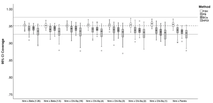
1. The range restriction on the distribution of the correlation ...17 2. Comparison between HPDI and Percentile-Based CIs ...28 3. Distributions considered for this study ...34 4. Distribution of 95% CI coverage for correlation magnitude. Fisher z-transformation

(FSH), percentile bootstrap (PB), bias-corrected and accelerated bootstrap (BCa), and highest probability density interval (HPDI). Bootstrap methods (PB, BCa, HPDI) were based on 2,000 bootstrap samples. The dashed line is at .95 and the solid lines are at



.925, . 975 ; acceptable coverage. ...95



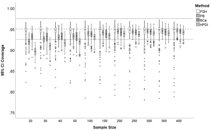
5. Distribution of 95% CI coverage for sample size. Fisher z-transformation (FSH),

percentile bootstrap (PB), bias-corrected and accelerated bootstrap (BCa), and highest probability density interval (HPDI). Bootstrap methods (PB, BCa, HPDI) were based on 2,000 bootstrap samples. The dashed line is at .95 and the solid lines are at



.925, . 975 ;



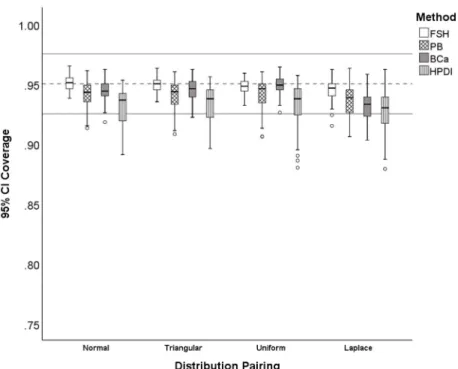
acceptable coverage. ...96 6. Distribution of 95% CI coverage for symmetric with symmetric distribution pairings.

Fisher z-transformation (FSH), percentile bootstrap (PB), bias-corrected and accelerated bootstrap (BCa), and highest probability density interval (HPDI). Bootstrap methods (PB, BCa, HPDI) were based on 2,000 bootstrap samples. The dashed line is at .95 and the solid lines are at





7. Distribution of 95% CI coverage for non-symmetric with non-symmetric distribution

pairings. Fisher z-transformation (FSH), percentile bootstrap (PB), bias-corrected and accelerated bootstrap (BCa), and highest probability density interval (HPDI). Bootstrap methods (PB, BCa, HPDI) were based on 2,000 bootstrap samples. The dashed line is

at .95 and the solid lines are at





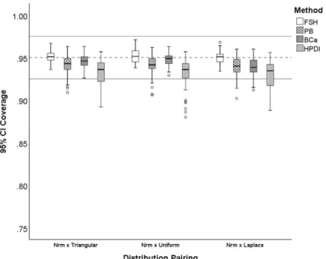
8. Distribution of 95% CI coverage for symmetric with normal distribution pairings.

Fisher z-transformation (FSH), percentile bootstrap (PB), bias-corrected and accelerated bootstrap (BCa), and highest probability density interval (HPDI). Bootstrap methods (PB, BCa, HPDI) were based on 2,000 bootstrap samples. The dashed line is at .95

(9)

9. Distribution of 95% CI coverage for non-symmetric with normal distribution pairings. Fisher z-transformation (FSH), percentile bootstrap (PB), bias-corrected and accelerated bootstrap (BCa), and highest probability density interval (HPDI). Bootstrap methods (PB, BCa, HPDI) were based on 2,000 bootstrap samples. The dashed line is at .95 and the solid lines are at





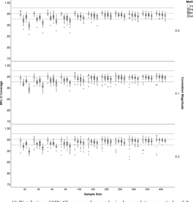
10.Distribution of 95% CI coverage for sample size by correlation magnitudes of 0 .2 .

and the solid lines are at





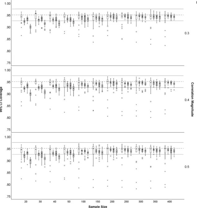
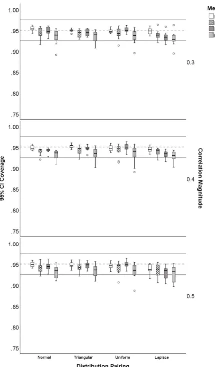
11.Distribution of 95% CI coverage for sample size by correlation magnitudes of .3 .5 .





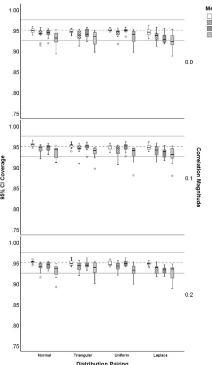
12.Distribution of 95% CI coverage for symmetric with symmetric distribution pairings by

correlation magnitudes of 0 .2 . Fisher z-transformation (FSH), percentile bootstrap (PB), bias-corrected and accelerated bootstrap (BCa), and highest probability density interval (HPDI). Bootstrap methods (PB, BCa, HPDI) were based on 2,000 bootstrap samples. The dashed line is at .95 and the solid lines are at



.925, . 975 ; acceptable



coverage. ...103 13.Distribution of 95% CI coverage for symmetric with symmetric distribution pairings by

correlation magnitudes of .3 .5 . Fisher z-transformation (FSH), percentile bootstrap (PB), bias-corrected and accelerated bootstrap (BCa), and highest probability density interval (HPDI). Bootstrap methods (PB, BCa, HPDI) were based on 2,000 bootstrap samples. The dashed line is at .95 and the solid lines are at





coverage. ...104 14.Distribution of 95% CI coverage for non-symmetric with non-symmetric distribution

pairings by correlation magnitudes of 0 .2 . Fisher z-transformation (FSH), percentile bootstrap (PB), bias-corrected and accelerated bootstrap (BCa), and highest probability density interval (HPDI). Bootstrap methods (PB, BCa, HPDI) were based on 2,000 bootstrap samples. The dashed line is at .95 and the solid lines are at



.925, . 975 ;



(10)

15.Distribution of 95% CI coverage for non-symmetric with non-symmetric distribution pairings by correlation magnitudes of .3 .5 . Fisher z-transformation (FSH), percentile bootstrap (PB), bias-corrected and accelerated bootstrap (BCa), and highest probability density interval (HPDI). Bootstrap methods (PB, BCa, HPDI) were based on 2,000 bootstrap samples. The dashed line is at .95 and the solid lines are at



.925, . 975 ;



acceptable coverage. ...106 16.Distribution of 95% CI coverage for symmetric with normal distribution pairings by

correlation magnitudes of 0 .2 . Fisher z-transformation (FSH), percentile bootstrap (PB), bias-corrected and accelerated bootstrap (BCa), and highest probability density interval (HPDI). Bootstrap methods (PB, BCa, HPDI) were based on 2,000 bootstrap samples. The dashed line is at .95 and the solid lines are at





coverage. ...107 17.Distribution of 95% CI coverage for symmetric with normal distribution pairings by

correlation magnitudes of .3 .5 . Fisher z-transformation (FSH), percentile bootstrap (PB), bias-corrected and accelerated bootstrap (BCa), and highest probability density interval (HPDI). Bootstrap methods (PB, BCa, HPDI) were based on 2,000 bootstrap samples. The dashed line is at .95 and the solid lines are at





coverage. ...108 18.Distribution of 95% CI coverage for non-symmetric with normal distribution pairings

by correlation magnitudes of 0 .2 . Fisher z-transformation (FSH), percentile bootstrap (PB), bias-corrected and accelerated bootstrap (BCa), and highest probability density interval (HPDI). Bootstrap methods (PB, BCa, HPDI) were based on 2,000 bootstrap samples. The dashed line is at .95 and the solid lines are at





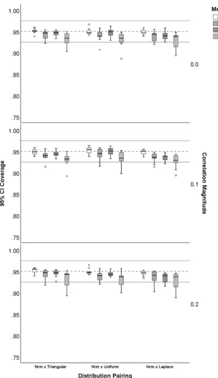
coverage. ...109 19.Distribution of 95% CI coverage for non-symmetric with normal distribution pairings

by correlation magnitudes of .3 .5 . Fisher z-transformation (FSH), percentile bootstrap (PB), bias-corrected and accelerated bootstrap (BCa), and highest probability density interval (HPDI). Bootstrap methods (PB, BCa, HPDI) were based on 2,000 bootstrap samples. The dashed line is at .95 and the solid lines are at





sample size of 20 40 . Fisher z-transformation (FSH), percentile bootstrap (PB), bias-corrected and accelerated bootstrap (BCa), and highest probability density interval (HPDI). Bootstrap methods (PB, BCa, HPDI) were based on 2,000 bootstrap samples.

(11)

21.Distribution of 95% CI coverage for symmetric with symmetric distribution pairings by sample size of 50 150 . Fisher z-transformation (FSH), percentile bootstrap (PB), bias-corrected and accelerated bootstrap (BCa), and highest probability density interval (HPDI). Bootstrap methods (PB, BCa, HPDI) were based on 2,000 bootstrap samples.

The dashed line is at .95 and the solid lines are at





22.Distribution of 95% CI coverage for symmetric with symmetric distribution pairings by

sample size of 200 300 200-300. Fisher z-transformation (FSH), percentile bootstrap (PB), bias-corrected and accelerated bootstrap (BCa), and highest probability density interval (HPDI). Bootstrap methods (PB, BCa, HPDI) were based on 2,000 bootstrap samples. The dashed line is at .95 and the solid lines are at









24.Distribution of 95% CI coverage for non-symmetric with non-symmetric distribution

pairings by sample size of 20 40 . Fisher z-transformation (FSH), percentile bootstrap (PB), bias-corrected and accelerated bootstrap (BCa), and highest probability density interval (HPDI). Bootstrap methods (PB, BCa, HPDI) were based on 2,000 bootstrap samples. The dashed line is at .95 and the solid lines are at











.925, . 975 ;



(12)

27.Distribution of 95% CI coverage for non-symmetric with non-symmetric distribution pairings by sample size of 350 400 . Fisher z-transformation (FSH), percentile bootstrap (PB), bias-corrected and accelerated bootstrap (BCa), and highest probability density interval (HPDI). Bootstrap methods (PB, BCa, HPDI) were based on 2,000 bootstrap samples. The dashed line is at .95 and the solid lines are at





coverage. ...118 28.Distribution of 95% CI coverage for symmetric with normal distribution pairings by





29.Distribution of 95% CI coverage for symmetric with normal distribution pairings by













32.Distribution of 95% CI coverage for non-symmetric with normal distribution pairings

by sample size of 20 40 . Fisher z-transformation (FSH), percentile bootstrap (PB), bias-corrected and accelerated bootstrap (BCa), and highest probability density interval (HPDI). Bootstrap methods (PB, BCa, HPDI) were based on 2,000 bootstrap samples.





(13)

34.Distribution of 95% CI coverage for non-symmetric with normal distribution pairings by sample size of 200 300 . Fisher z-transformation (FSH), percentile bootstrap (PB), bias-corrected and accelerated bootstrap (BCa), and highest probability density interval (HPDI). Bootstrap methods (PB, BCa, HPDI) were based on 2,000 bootstrap samples.









36.Distribution of standardized bias for correlation magnitude. Ranked inverse normal

(RIN). The dashed line is at 0 and the solid lines are at



.40, .40



; acceptable bias. ...127 37. Distribution of standardized bias for sample size. Ranked inverse normal (RIN). The

dashed line is at 0 and the solid lines are at



.40, .40



; acceptable bias. ...128 38.Distribution of standardized bias for symmetric with symmetric distribution pairings.

Ranked inverse normal (RIN). The dashed line is at 0 and the solid lines are at



.40, .40



; acceptable bias. ...129 39.Distribution of standardized bias for non-symmetric with non-symmetric distribution

pairings. Ranked inverse normal (RIN). The dashed line is at 0 and the solid lines are

at



.40, .40



; acceptable bias. ...130 40.Distribution of standardized bias for symmetric with normal distribution pairings.



.40, .40



; acceptable bias. ...131 41.Distribution of standardized bias for non-symmetric with normal distribution pairings.



.40, .40



; acceptable bias. ...132 42.Distribution of standardized bias for sample size by correlation magnitude of 0 .2 .



.40, .40



; acceptable bias. ...133 43.Distribution of standardized bias for sample size by correlation magnitude of .3 .5 .

(14)

44.Distribution of standardized bias for symmetric with symmetric distribution pairings by correlation magnitude of 0 .2 . Ranked inverse normal (RIN). The dashed line is

at 0 and the solid lines are at



.40, .40



; acceptable bias. ...135 45.Distribution of standardized bias for symmetric with symmetric distribution pairings

by correlation magnitude of .3 .5 . Ranked inverse normal (RIN). The dashed line is



.40, .40



pairings by correlation magnitude of 0 .2 . Ranked inverse normal (RIN). The dashed line is at 0 and the solid lines are at



.40, .40



pairings by correlation magnitude of .3 .5 . Ranked inverse normal (RIN). The dashed line is at 0 and the solid lines are at



.40, .40



; acceptable bias. ...138 48.Distribution of standardized bias for symmetric with normal distribution pairings by

correlation magnitude of 0 .2 . Ranked inverse normal (RIN). The dashed line is at

0 and the solid lines are at



.40, .40



correlation magnitude of .3 .5 . Ranked inverse normal (RIN). The dashed line is at 0



.40, .40



; acceptable bias. ...140 50.Distribution of standardized bias for non-symmetric with normal distribution pairings

by correlation magnitude of 0 .2 . Ranked inverse normal (RIN). The dashed line is



.40, .40



by correlation magnitude of .3 .5 . Ranked inverse normal (RIN). The dashed line is



.40, .40



by sample size of 20 40 . Ranked inverse normal (RIN). The dashed line is at 0 and

the solid lines are at



.40, .40



(15)

54.Distribution of standardized bias for symmetric with symmetric distribution pairings by sample size of 200 300 . Ranked inverse normal (RIN). The dashed line is at 0 and the solid lines are at



.40, .40



; acceptable bias. ...145 55.Distribution of standardized bias for symmetric with symmetric distribution pairings by

sample size of 350 400 . Ranked inverse normal (RIN). The dashed line is at 0 and the solid lines are at



.40, .40



pairings by sample size of 20 40 . Ranked inverse normal (RIN). The dashed line is



.40, .40



pairings by sample size of 50 150 . Ranked inverse normal (RIN). The dashed line is at 0 and the solid lines are at



.40, .40





.40, .40





.40, .40



sample size of 20 40 . Ranked inverse normal (RIN). The dashed line is at 0 and the

solid lines are at



.40, .40





.40, .40



sample size of 200 300 . Ranked inverse normal (RIN). The dashed line is at 0 and



.40, .40





.40, .40



; acceptable bias. ...154

(16)

64.Distribution of standardized bias for non-symmetric with normal distribution pairings by sample size of 20 40 . Ranked inverse normal (RIN). The dashed line is at 0 and the solid lines are at



.40, .40





.40, .40



by sample size of 200 300 . Ranked inverse normal (RIN). The dashed line is at 0 and the solid lines are at



.40, .40



by sample size of 350 400 . Ranked inverse normal (RIN). The dashed line is at 0 and the solid lines are at



.40, .40



; acceptable bias. ...158

(17)

CHAPTER I INTRODUCTION

Scientific research is conducted to create a deeper understanding of a discipline for its advancement. In the behavioral sciences, this means creating theories that allow for a better understanding of human behavior and potentially making it predictable. A way to find support for the validity of these theories is to demonstrate consistent result replication across research. However, a collaboration of researchers that attempted to replicate 100 scientific studies found a less than 50% replication rate (Collaboration, 2015). Specifically, the replication rate was 36% for studies that used p-values and 47% for studies that used effect sizes with confidence intervals (CIs). These results are far from ideal and do not garner much confidence.

There are many potential causes for the low replication rate in the Collaboration (2015) study; however, the authors suggest that publication, selection, and reporting biases are major contributors. In this sense, the results reflect a research climate that incentivizes research that is “statistically significant,” which creates a bias on what kind of research is conducted and how it is reported (Ioannidis, 2005). There have been multiple suggestions to address these issues, but they have been met with some contention and other issues. One suggestion is to further lower the

p-value threshold for declaring statistical significance to curb researchers from gaming the system for specific outputs (Benjamin, 2017). However, technological advancements have made gathering large samples much easier than what was possible in the past. As such, lowering the

p-value criteria for statistical significance may not be enough. Another approach would be to instead directly address the tools and methods used.

An upfront suggestion from this approach would be to use effect sizes in addition to statistical significance (Cohen, 1990). As shown from the 36% to 47% replication rate jump in

(18)

the Collaboration (2015) study, this latter approach shows promise. Even so, this suggestion can further be enhanced by including confidence intervals (CIs) for effect sizes to provide precision information.

Along this line of discussion, a popular statistic that can also play the role of an effect size is the correlation. In fact, the correlation was the effect size measure used in the majority of studies in the Collaboration (2015) study. The correlation can take on several forms, but the original Pearson product-moment correlation (henceforth referred to as the correlation) is the most iconic with over 100 years of use (Hald, 2007). Additionally, the correlation is foundational to many other statistics and statistical models like the t-test, regression, MANOVA, etc. Given the ubiquity of the correlation, its importance to other statistics, and its use as an effect size, CI research about the correlation is essential. This is especially true if effect sizes are being proposed as a method to help with research replication.

However, CI research about the correlation is limited with contradictory results. Some research shows that the correlation and its CIs are robust to non-normal data and others demonstrate the opposite. The focus on non-normal data is important as there is evidence to suggest that non-normal data is common (Blanca et al., 2013). Furthermore, much of the research is focused on the null hypothesis of when the correlation is zero (



0). This kind of

information is not entirely relevant to situations that call for the use of the correlation as an effect size; i.e., situations where the correlation does not equal zero (



0). Therefore, the research here will address this gap by investigating bootstrap CIs for the correlation when



0,



0, and non-normal data. This will also include an exploration of a CI method that has not been previously explored. However, this discussion begins with concept of “statistical significance” and its relation to CIs.

(19)

Null Hypothesis Significance Testing

The most prevalent form of hypothesis testing is null hypothesis significance testing (NHST). In fact, the 36% replication rate for p-values of studies in the Collaboration (2015) study is based on NHST. Classically and at its simplest, NHST is conducted by setting up two opposing hypotheses: the null

 

H0 and alternative

 

HA hypotheses. In NHST,

H

0 is assumed to be true (e.g., no effect or no relationship), but data is used to test this claim (Perezgonzalez, 2016). This process requires selecting a criterion (α) that establishes a low probability threshold within

H

0 occurring and compares this criterion to the probability of obtaining an effect (p-value) from the data. Within this context, α is the probability of rejecting a true

H

0 (i.e., the probability of a type I error). If the p-value is less than α, then

H

0 is rejected in support of

A

H

(e.g., the effect is statistically significant). As such, the principle idea of statistical

significance is to demonstrate that obtaining an observed effect would be highly unlikely if

H

0 is true (Fisher, 1929).

Since NHST only establishes the probability of obtaining an effect when assuming that 0

H

is true, it restricts p-values to only being able to infer the compatibility of an effect to

H

0. A common misconception is that the p-value is the probability of

H

₀ being true given an effect (Cohen, 1994). This confusion is further compounded by the misinterpretation that the

complement of the p-value (1p) is the probability of

H

Abeing true (Nickerson, 2000). This has led to inaccurate reporting of p-values such that there is a belief that a p



is associated with a greater than 100(1



)% chance of

H

A being true. For example, a p.05 is interpreted as a greater than 95% chance of

H

_A being true. While these misinterpretations may not be

(20)

directly caused by NHST, they illustrate the downward spiral of confusion that results from misunderstanding a tool (e.g., NHST in this context).

This is not to say that NHST is limited strictly due to misconceptions or less than noble intentions. Another way to think about NHST is that it only informs researchers how well an effect relates to a hypothesis in terms of probability. For example, say that a test for mean difference has a p.03. If  .05, then the test is statistically significant. However, if  .01, the test is not statistically significant. Thus, the results of NHST can change depending on the α

level used to analyze an effect (Wasserstein & Lazar, 2016). Additionally,

H

0 is assumed to be equal to a specific value (e.g.,

H

0

:

 

1



2



0

), and any deviation from this value would demonstrate that

H

0 is not true.

Consider a test of mean difference (i.e., the effect) between a group of participants before and after a treatment where

H

0 is stated as “There is no mean difference before and after a treatment” (i.e.,



_D



0

) and  .05. The descriptive statistics for this example are: n10, mean difference is

M

_D



3

, and the variance of the difference is _S2 _₂₂₅_{. A related-samples}

t-test of this data would be

2 3 0.6325 225 10 D D M t S n    (1.1)

where the denominator is the standard error (SE). This effect is not statistically significant at .05

  which has tcrit 2.2622. If this example were modified by increasing n to 100 (i.e., 100

(21)

2 3 2 225 100 D D M t S n    . (1.2)

This is statistically significant at  .05 which now has tcrit 1.9842. This demonstrates that by increasing the sample size, statistical significance can be obtained by way of decreasing the associated critical value. Note that this occurred despite no change in the mean difference (i.e., the effect) or the variance of the difference. Although presented in an idealistic manner, sample size can impact statistical significance in other ways. For example, increasing the sample size typically decreases variance, which in turn again increases statistical significance. Even so, statistical significance can be obtained by simply increasing the sample size because it decreases the corresponding critical value; a relationship that holds for any form of NHST. This is key as modern technological advancements make obtaining larger sample sizes, and by extension statistical significance, easier than what was possible in the past. Furthermore, the results of statistical significance do not inform in terms of precision and a standard (or common) scale, which makes interpretations of NHST results even more cumbersome. To address the precision limitations of statistical significance, interval estimation should be used about the parameter of interest in NHST.

Interval Estimation and Confidence Intervals

There are two general methods for estimating a parameter: point and interval. A point estimate uses a single value for a parameter estimate. Examples of point estimates are the mean and variance for the difference (e.g.,

M

Dand SD2 ). A point estimate is useful for establishing a

best guess for a parameter but does not account for sampling error (or variability) about the parameter estimate. However, an interval estimate consists of a range of possible values that are

(22)

likely to contain the population parameter. Interval estimates manifest this range by accounting for error to provide precision information about estimating the parameter of interest.

A common application of interval estimation is the confidence interval (CI). Assuming a random sample from a given distribution, a CI is formed by creating an error structure around a point estimate based on the standard error (SE) of the corresponding distribution with a

confidence level (Hogg, Tanis, & Zimmerman, 2015). A confidence level indicates the consistency of a parameter estimate and is denoted as 100(1



)% where α represents the probability of making a type I error. In the context of a CI with  .05 , a 95% CI indicates an expectation that 95% of all CIs created in the same way will contain the corresponding

population parameter.

Besides providing information about the precision of a parameter estimate, CIs also have utility in hypothesis testing. In these cases, statistical significance is met when the parameter specified under

H

0 is not within the bounds of the CI. Conversely, having a CI that contains the parameter for

H

₀ indicates support for

H

₀.

A CI for a related-samples t-test can be constructed as follows:

/2 D₂ /2 1 D M P t t S n        _ _ _ _{ }       , (1.3) 2 2 /2 D , /2 D D D S S M t M t n n          _ _  _ _  _ _ _ _   , (1.4) 2 /2 D D S M t n     _ _  , (1.5)

(23)

and

1

df  n (1.6)

where

t

/2 refers to the t-critical value associated with probability of making a type I error divided by 2. The division of α by 2 is used in this context to create a CI with endpoints around the estimate.

Continuing with the previous two related-samples t-test examples. The first example has 10

n with df 9 and the corresponding 95% CI using equation 1.5 is estimated as

225 3 2.262 10    __ __   (1.7)

and



7.7296, 13.7296



. The second example has n100 with df 99 and the corresponding 95% CI using equation 1.5 is 225 3 1.984 100    __ __   (1.8)

and



0.0240, 5.9760 . In the first case, since the CI includes



H

0 (i.e.,



D



0

), the result is not significant. In the second case, the CI does not include

H

₀ and is significant. In terms of statistical significance, these CIs provide the same information as the original examples. However, because CIs incorporate sampling error through the SE, precision information

regarding the parameter is provided (



D in this case). Nevertheless, the limitation with respect to replication is that CIs are not in a standard (or common) scale because the parameter (or effect) is not in standard scale.

NHST only establishes if a parameter (or effect) is significant with respect to a hypothesis, and a CI provides the same information but adds precision information about the

(24)

parameter (or effect). Neither lends credence as to whether the effect is meaningful; only that an effect is detected and how well it is estimated. When statistical significance is found under NHST, effects of 1, 10, .001, etc. can all hold equal value to the result (Tukey, 1991). This is because there is no sense of scale inherit to NHST due to the binary nature of the result; it only matters that the effect is different from what is stated in

H

0. A CI only adds precision

information about the effect; i.e., it gives information about how well the parameter is estimated. So while an effect of .001 may be statistically significant and may be estimated well, it is

difficult to judge if this effect has more real-world weight compared to similar effects from different research (i.e., practically significant). These limitations in clarity demonstrate that other methods should be used that can better demonstrate the utility of an effect. This leads to effect sizes.

Effect Sizes

An effect size is a statistic that measures the magnitude of an effect. The utility of an effect size over NHST is that it explains an effect in terms of a standard (or common) scale rather than the original units of measurement (Cohen, 1988). This means that regardless of the

statistical significance of an effect and/or how well it is estimated, the effect can be easily and consistently understood. For example, an effect size that ranges from 0 to 1 can be understood to have greater effect as the effect approaches 1. Furthermore, this process can be extended to compare studies in terms of effect size magnitudes. The utility has been acknowledged and has led to the consideration of reporting effect sizes as a standard (Wilkenson, 1999).

Consider again the previous two mean difference examples. One kind of effect size appropriate here is Cohen’s d (Cohen, 1988). Cohen suggests the following guidelines for

(25)

judging the magnitude of d: 0.20, 0.50, and 0.80 are small, medium, and large effects, respectively. In this situation, the effect size is

2 3 0.1875 256 D D M d S    (1.9)

which is considered a small effect. The key thing to notice is that, regardless of statistical significance and precision, both examples have the same effect size. This occurs because

Cohen’s d only compares the ratio of the effect to error (or variance) without considering sample size. Unlike statistical significance and precision, sample size has little or no impact on effect sizes (Sullivan & Richard, 2012). Therefore, a strict reliance on “statistical significance” does not provide enough information to make proper conclusions about an effect and the example highlights the difference between statistical and practical significance. However, this issue can be alleviated through effect size use.

At this point, it is clear why some researchers suggest using effect sizes in additional to statistical significance (Cohen, 1990). An effect size is less impacted by sample size and puts the effect on a standard (or common) scale. Additionally, they can be used to compare the results from different studies (e.g., meta-analysis). As such, effect sizes help provide a more complete picture for the results found in hypothesis testing. However, effect sizes would have more utility if they had precision information. This can be achieved by forming effect size CIs and would allow researchers to know how well their effects are estimated. Of current contention related to this are CIs about the correlation as CI research regarding the correlation is limited and mixed. The Pearson Correlation as an Effect Size

As aforementioned, the Pearson product-moment correlation (or correlation for short) is a popular statistic that can also play the role of an effect size. The popularity and importance of the

(26)

correlation stems from its over 100 years of use and its contribution as a foundational piece to other statistics and statistical models like the t-test, regression, MANOVA, etc. (Hald, 2007). Additionally, the correlation was the effect size used in most of the replication studies in the Collaboration (2015) study. Like any effect size, sample size has little to no impact on the correlation and a CI for it would also let researchers know how well the correlation was

estimated. However, CI research for the correlation is sparse with varied results. Therefore, the research here will address this gap by evaluating non-bootstrap and bootstrap CIs for the correlation.

The correlation is a method used to measure the linear relationship between two variables. In population settings, the correlation for variables x and y is defined as

xy xy x y





 

 (1.10)

where, and



_xy is the covariance between x and y, and



x and



y are the standard deviations

for the x and y, respectively. When dealing with samples, the parameters are replaced with their respective estimates and equation 1.10 becomes

xy xy x y s r s s  (1.11)

With this structure, it can be understood that the correlation is a ratio between how the x and y

variables vary together. Another way to think of this is how much the variation in x is related to variation in y and vice versa.

The correlation has a range of   1



1. This results in a standard (or common) scale where a correlation of 1 indicates a perfect-positive relationship, -1 a perfect-negative

(27)

interpretations. In this context, “perfect-positive” indicates that as one variable increases the other variable will invariably match that increases in the same direction while a

“perfect-negative” indicates that as one variable increases the other will invariably match that increase in the opposite direction. Cohen (1988) suggested the following guidelines for judging the magnitude of r: 0.10 , 0.30 , 0.50 are small, medium, and large effects, respectively. The simplicity in implementation and interpretation lends to the correlation’s popularity and allows the correlation to serve as a scaffolding piece to other statistics like the coefficient of

determination.

The coefficient of determination

 

_r2 _{is another effect size directly related to correlation} as it is just the correlation squared and is defined as

2 2 2 2 xy x y      (1.12) or 2 2 2 2 xy x y s r s s  (1.13)

depending on whether populations or samples are used, respectively. Like the correlation, r2_can

be thought of as a proportion. In this case, it is the proportion of variance in either variable that is accounted for by the other (Cohen, 1988). This concept can be extended to linear models. For example, r2_{is the amount of variability in the outcome (}_y_{) accounted for by a linear regression}

model. The purpose of making this connection is to note that the correlation is integral to other statistics and that correlation’s qualities and interpretations will propagate to those other statistics that are dependent on the correlation.

(28)

To summarize, replication of research findings is a concern in scientific research

(Collaboration, 2015). In response, one suggestion is to lower the p-value threshold for declaring statistical significance (Benjamin, 2017). However, modern technological advancements (e.g., statistical computing, online surveys, etc.) have made gathering large amounts of data easy. Therefore, in addition to reporting statistically significant findings, researchers have also

suggested reporting effect size measures as they are minimally impacted by sample size (Cohen, 1990). This suggestion shows promise as effect sizes had a higher replication rate than statistical significance in a collaborative study (Collaboration, 2015). Even so, this suggestion can further be enhanced by including CIs for effect sizes to provide effect size precision information. One common effect size is the correlation (ρ) and was in fact the effect size used in the majority of the studies in the collaborative study. However, CI research about the correlation or its

robustness is limited, and in some cases conflicting. Research regarding the robustness of correlation is now discussed.

Robustness of the Correlation t-test

Early research regarding the robustness of the correlation primarily focused on the application of the t-test for testing



0. An early study of this kind of robustness was done by Blair and Lawson (1982). The authors main contention with previous work was its limitations to familiar distribution shapes that may not be reflective of “actual research contexts” where non-normal data is more common (Kowalski, 1972; Norris & Hjelm, 1961; Pearson &

Adyanthaya, 1929). As such, the authors investigated a severely non-normal distribution (i.e., the Bradley distribution with skew = 3 and kurtosis = 17). For distribution shape, the distribution was the same for both variables. This simulation study investigated the impact of (a) distribution shape (normal and Bradley) and (b) sample size (n5, 30, 50,100) on the type I error rate of the

(29)

correlation t-test for testing



0. Results were based on 5,000 simulation replications and

.005, .01, .025, and .05



 . The results indicated that the correlation t-test type I error rate was accurate under the normal distribution but had inflated type I error rate under the Bradley distribution. Additionally, increasing the sample size did not help and appeared to make the situation worse for the Bradley distribution. Results across α were generally consistent.

In a subsequent study, Edgell and Noon (1984) examined the type I error rate for the correlation t-test when testing



0. This was done by investigating (a) distribution shape, (b) distribution pairing, and (c) sample size (n5,10,15, 20, 30, 50,100) for



.01and .05. The primary interest of this research was to determine how the correlation t-test responds to

non-normal distributions. The distributions investigated were:

 Normal (skewness = 0, kurtosis = 0)

 Uniform (skewness = 0, kurtosis = -1.2)

 Exponential (skewness = 2.07, kurtosis = 6.56)

 Cauchy Form 1 (skewness = 21.56, kurtosis = 2171)

 Cauchy Form 2 (skewness = 49.8, kurtosis = 2817.9)

These distributions were then either paired with themselves or with another distribution (i.e., all pairwise combinations) resulting in a total of 15 distribution pairing being explored. Results were based on 10,000 simulation replications. The results of this study showed that the t-test for testing



0 is robust at controlling type I error at  .05 and when n5. However, it was not robust for extreme distributions (e.g., Cauchy) at  .01.

Early research on the robustness of the correlation is limited and mixed. According to some of the research, the correlation t-test is robust when testing that the population correlation

(30)

is zero (



0). However, some of the research indicates that this is not the case when working with severely non-normal data. This is concerning as data typically encountered in research environments is non-normal (Blanca et al., 2013). Furthermore, even if the research showed clear evidence that the correlation t-test is robust to distributional assumptions when testing that

0



 , these results would bear little information about estimating the correlation when



0. When the correlation hypotheses are of the form H0:



0 vs. HA:



0, rejecting H0 only

indicates that



0 is an unlikely event and provides no information about estimating



0. As such, if using the correlation as an effect size is of interest, then testing



0 has little utility. It would be of greater interest to investigate the correlation across its range ( 1  



1). A way to investigate this is through CIs for the correlation.

Confidence Interval Research About the Correlation

One early attempt to investigate estimating correlation CIs when



0 was the Fisher

z-transformation (Fisher, 1915). The Fisher z-transformation is defined as

1 1 ln 2 1 r z r         _{  } _ _. (1.14)

This allows for a 100(1



)% CI to be defined as

 

/ 2 z z _ SE z , (1.15) where

 

1 3 SE z n   (1.16)

(31)

Zeller and Levine (1974) evaluated the performance of the Fisher z-transformation CI for the correlation from equations 1.14 to 1.16 under several simulation conditions. The authors investigated the (a) distribution shape, (b) correlation strength (



0, .32, .71, .95), and (c) sample size (n15, 50,100) for



.01and .05. For distribution shape, the distribution was the same for both variables and the authors investigated the normal, uniform, J, bimodal, and a leptokurtic, but provided no skewness and kurtosis details for these distributions. Results were based on 3,000 simulation replications. One consistent finding was that the estimate of the correlation from equation 1.11 slightly underestimated the true correlation, but this was

ultimately negligible when n 15. In addition, the correlation CI from equation 1.15 was shown to be robust to the mild non-normal distributions investigated (e.g., uniform, J, bimodal, and leptokurtic). These results were consistent for



.01and .05.

Additional research on the robustness of the Fisher z-transformation CI for the correlation was conducted by Berry and Mielke (2000). The authors investigated (a) distribution shape, (b) correlation strength (



0, .4, .6, .8), and (c) sample size (n10, 20, 40,80) for

.10 .05, and .01



 . For distribution shape, the distribution was the same for both variables and the authors investigated were the normal, 3 generalized logistic, and 3 symmetric kappa

distributions. The generalized logistic distributions were defined by

 

1/ 1  1 / x x e e f x              _ _{ }  _     (1.17)

where



1,.1,.01. In this context,  1 results in negative skew and  1 results in positive skew. The symmetric kappa distribution was defined by

(32)

 1 / 1/ ( ) .5 1 x f x    



       _ _   (1.18)

where



2,3,25. In this context,  2 represents a distribution similar to a t distribution with 2 degree of freedom,  3 a distribution with heavy tailed distribution, and  25 is similar to a uniform distribution with thin tails. The authors provided no skewness and kurtosis details for these distributions. Results were based on 1,000,000 simulation replications. The results showed that Fisher z-transformation CIs have appropriate coverage probability when  .05 and



0

for all distribution shapes. However, the coverage probability was consistently underestimated when distribution shapes are non-normal and



0. Furthermore, these problems were not remedied with increased sample size but made more severe. These results were consistent for

.01.05, and .10



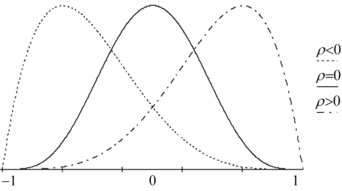
 This discrepancy in the literature about the efficacy of correlation CI methods indicate the need for additional research on the matter.

The issue with correlation CI research is the   1



1 range restriction on the correlation (See Figure 1; Blanca et al., 2013). This range restriction makes estimating the correlation when



0 difficult as the correlation becomes more skewed as it approaches ±1. In fact, the only time the correlation is symmetric is when



0. As such, it is apparent that estimating the correlation CIs is difficult when



0. However, the bootstrap is a powerful method that can be used for CI estimation of the correlation without making distributional assumptions.

(33)

Figure 1. The range restriction effect on the distribution of the correlation.

Bootstrap Method

Bootstrapping is a statistical technique that uses data to create simulations for statistical inference (Efron & Tibshirani, 1993). This method generates the sampling distribution of a parameter estimate through sampling with replacement from a sample. This generated sampling distribution can be used to obtain SEs, CIs, and do hypothesis testing. The bootstrap method has two distinct advantages over parametric methods. First, it is a robust alternative used when parametric based inference is in doubt (e.g., the normality assumption is in doubt). Second, bootstrapping is a good alternative when parametric inference is impossible or requires very complicated equations for

(34)

An important detail about the bootstrap method is that it can be used to estimate the sampling distribution of almost any statistic without any prior knowledge of its sampling distribution. To understand this, consider the Central Limit Theorem (CLT) and the mean (μ). The CLT states that regardless of the population distribution of a sample, the sampling

distribution of the sample mean (M) will approach normality as n approaches infinity. In this case, the bootstrap method can simulate the CLT by providing an estimate of the sampling distribution of the statistic (i.e., the empirical sampling distribution or ESD). This also allows for

SE estimates (i.e., the standard deviation of the sampling distribution) once the ESD is generated. This means that the bootstrap method can be used as a brute force way to estimate the SE of almost any statistic.

Consider an example where a sample x is obtained of size n and the mean is of interest. This sample is defined as x



x x₁, , ...,₂ x_n



. The bootstrap is then performed in three steps. First, obtain the _bth_{random sample with replacement from}_x_{; i.e.,}  



     



1 , 2 ,...,

b b b b

n

x  x x x . Second, compute and store the _bth_{estimate of the mean}

 

_M b _from_x b

. Third, compile the stored estimates

M

(1)

,

M

(2)

, ,



M

( )B

to create the ESD of M for the b1, 2, ...,B bootstrap samples. The bootstrap estimate of the SE is defined as

 





2 ( ) 1 1 B b i M M SE M B    



(1.19) where ( ) 1 1 B b b M M B  



(1.20)

(35)

is the mean of the ESD. The implication of this example is that this process can be extended to other statistics without knowledge of the corresponding sampling distributions (e.g., the correlation).

As aforementioned, the bootstrap method can be used to estimate the SE and that allows for CI estimation. Using the previous example, a CI for the mean can be estimated by

 

/ 2

M z SE M_ . (1.21)

Note the similarities between equations 1.5 and 1.21. A limitation of equation 1.21 is that it requires knowledge of the sampling distribution; in this case, knowledge that the sampling distribution is normal. The bootstrap overcomes this limitation by offering two alternative CIs that do not require this knowledge; the percentile and bias-corrected and accelerated CIs. Percentile Bootstrap CI

The percentile bootstrap (PB) CI is a distribution-free method for constructing bootstrap CIs based on the percentiles of the ESD. In the context of the previous mean example, the PB CI is defined as 1 / 2 ( /2)_, B B M  M      (1.22) where ( / 2) B M  and (1 /2) B

M  _{are the α/2 and 1}___{/ 2}_{percentiles from the ESD and}_α_{is the} probability of type I error. For example, with 1000 bootstrap samples and  .05, 25 and 975 would serve as the percentiles of the ESD. The utility of the PB CI is that it is easy to understand and transformation respecting. This means that for a CI of ( /2)_, (1 /2)

B B

M  M 

 

  for µ, a

transformation t

 

 will have a corresponding CI of



( /2)

 

(1 /2)



,

B B

t M  t M 

 

(36)

Bootstrap Bias-Corrected and Acceleration CI

Another distribution-free method for creating bootstrap CIs is the bias-corrected and accelerated (BCa) method. This is like the PB CI method but also adjusts for bias and

acceleration. In this context, bias refers to the discrepancy between the bootstrap statistics and the corresponding sample statistic and acceleration refers to skew. If bias and acceleration are non-issues, then the PB and the BCa CIs methods yield similar results. This method also benefits from being transformation respecting but is also first and second order accurate. First and second order accurate means for a sample size n, the CI will have error that tends to zero at a rate of 1/ n and 1/n, respectively.

Continuing with the mean example, the BCa CI for M is defined as

1 2 ( )_, ( ) M  M      (1.23) where





0 ( ) 1 0 0 ( ) ˆ ˆ ˆ ˆ 1 z z z a z z     _   _     , (1.24)





0 (1 ) 2 0 0 (1 ) ˆ ˆ ˆ ˆ 1 z z z a z z       _        _ _    , (1.25)

Φ is the standard normal cumulative distribution function,

z

ˆ

0is bias, ˆa is acceleration, and

z

( ) and

z

(1) are the percentile cutoffs from the standard normal distribution. Bias is defined as





1 ( ) 0 1 1 ˆ B b b z I M M B       _  _ 



, (1.26)

(37)

where



1

 

.

is the inverse standard normal cumulative distribution function, I(.) is the indicator function, and M is the mean of the original data. Acceleration is accounted for by jackknife resampling where data are resampled by removing one observation per resample. Given data

x





x x

1

, ,...,

2

x

n



, the ith jackknife sample for i1, 2, ...,n is





( )i 1, 2, ..., i 1, i 1, ..., n

x  x x x_ x_ x (1.27)

with the _ith_{data point removed. Acceleration is defined as}









3 ( ) ( ) 1 3/2 2 ( ) ( ) 1 ˆ 6 n i i n i i M M a M M        _     



(1.28) where ( ) ( ) 1 1 n i i M M n   



(1.29)

and

M

( )i is the mean estimate that excludes the ith data point. Acceleration in this form is simply

the skewness multiplied by 1/6 and serves as a skewness correction factor.

An early application of the bootstrap CI for the correlation was presented by Lunneborg (1985). Lunneborg explored the potential of the bootstrap for estimating correlation CIs using SAT verbal and math scores from a pseudorandom sample of 25 college freshman. In this study, the PB CI, based on 500 bootstrap samples, was compared to the Fisher z-transformation CI from equation 1.14 and α was not disclosed. The SAT scores were used because (a) they are real data, (b) the verbal and math scores are known to be bivariate normal, and (c) the verbal-math ρ

(38)

is large enough so that useful CIs can be estimated for the small pseudorandom sample (n25). The CIs from both methods were similar under bivariate normality.

An early simulation study of the bootstrap CI for the correlation was conducted by Rasmussen (1987). Of interest was the impact of a non-normal distribution on the bootstrap CI for testing



0. This was done by investigating (a) distribution shape (normal and lognormal) and (b) sample size (n5,15, 30, 60) for



.01and .05. For distribution shape, the variable pairings for ρ took the following two forms: normal-normal or normal-lognormal. The PB CI, based on 500 bootstrap samples, was compared to the Fisher z-transformation CI. Results were based on 1,000 simulation replications. The results ran counter to Lunneborg’s research (1985) as they showed a lack of parity between the Fisher z-transformation and the PB CI. In this case, the PB CIs demonstrated an overall increase in type I error rate and restrictive CIs compared to the Fisher z-transformation CI under all conditions, including when the variable pairing was normal-normal. Going from  .05 to  .01 further highlights this issue. In addition,

Rasmussen noted that the situation did improve as sample size with larger sample sizes but was not able to explore this due to costs in computational power at the time.

In two recent studies, Padilla and Veprinksy (2012, 2014) developed PB and BCa CIs for the deattenuated correlation for  .05. An estimated correlation can become weaker

(attenuated) than what may be true in the population due to measurement error (Spearman, 1904). Spearman (1904) developed a correction for this attenuation known as the deattenuated (or disattenuated) correlation (Muchinsky, 1996), but research on this correlation and its corresponding CI is rare. Padilla and Veprinsky (2012, 2014) address this gap by investigating the bootstrap CIs for the deattenuated correlation under four simulation conditions: the (a)

(39)

variables in the correlation (



_ij .50, .60, .70, .80, .90), (d) and sample size

(n50,100,150, 200, 250, 300). All bootstrap CIs were based on 2,000 bootstrap samples. For distribution shape, both variables had the same distribution from the following distributions investigated:

 Normal (skewness = 0, kurtosis = 0)

 Uniform (skewness = 0, kurtosis = -1.20)

 Triangular (skewness = 0, kurtosis = -0.60)

 Beta (skewness = -0.85, kurtosis = 0.22)

 Laplace (skewness = 0, kurtosis = 3)

 Pareto (skewness = 2.81, kurtosis = 14.83)

Results were based on 1,000 simulation replications. Overall, the PB and BCa CIs had good coverage under all simulation conditions with negligible differences between the two CIs. Even so, the BCa CI tended to have slightly better coverage than the PB CI. The one exception was that neither CI performed well with the Pareto distribution. However, the Pareto distribution investigated was skewed and highly peaked (kurtosis = 14.83). Such distributions have range restrictions, and it is well known that distributions with range restrictions attenuate the correlation due to less variability.

In a subsequent study, Bishara and Hittner (2017) investigated several CIs for the correlation. Of interest was the impact of various types and combinations of distributions on the correlation CIs. The following correlation CIs were investigated: the 1) Fisher z-transformation, 2) Spearman rank-order with Fieller’s SE, 3) Spearman rank-order with Wright’s SE, 4)

Box-Cox transformation, 5) ranked inverse normal transformation, 6) nonparametric bootstrap, 7) nonparametric bootstrap with asymptotic adjustment (AA), 8) nonparametric bootstrap BCa,

(40)

9) observed imposed bootstrap, 10) observed imposed bootstrap with AA, and 11) observed imposed bootstrap with BCa. All bootstrap CIs were based on 9,999 bootstrap samples. The performance of the CIs was investigated through a simulation with the following four conditions: (a) distribution shape, (b) distribution pairing, (d) correlation strength (



0, .5), and (c) sample size (n10, 20, 40, 80,160) for  .05. The distributions investigated were a result of a

combination of population skewness

(



1

    

4, 3, 2, 1, 0,1, 2, 3, 4)

and kurtosis 2

(



 

1, 0, 2, 4, 6, 8,10, 20, 30, 40)

whose feasibility was limited by the lower bound of kurtosis being determined by the squared skewness

2 2 1 2







 . (1.30)

This resulted in 46 skewness and kurtosis combinations being investigated. The distribution pairing investigated either had both variables come from the same distribution or had one variable come from a normal distribution and the other from a non-normal distribution. Overall, 920 simulation scenarios were investigated. Results were based on 10,000 simulation

replications.

The primary findings were that the RIN followed by the Spearman rank-order with Fieller’s SE CIs had the best performance when data are non-normal. Of the remaining CI methods, only the observed imposed bootstrap with BCa had good enough performance when data was non-normal. However, it tended to exceed 95% coverage by generating somewhat long CIs. The advantage it has is that it keeps the correlation in the scale of the original variables. This is not the case for the RIN and Spearman rank-order with Fieller’s SE as both transform the original variables. All the remaining methods did not have good CI coverage when data were

(41)

non-normal with the Fisher z-transformation CI having the least favorable performance, and the situation was made worse by increasing the sample size when



.5.

When the variable pairing included a normal distribution, all CIs generally performed better. However, the transformation methods still outperformed the bootstrap methods in this case. The only bootstrap CI methods that was comparable to the transformation methods’ performance were the observed imposed bootstrap with AA and observed imposed bootstrap with BCa.

Like research on the robus