Transactions
[email protected] ISSN: 1696-2281
eISSN: 2013-8830 www.idescat.cat/sort/
Small area estimation of poverty indicators under
partitioned area-level time models
∗Domingo Morales1, Maria Chiara Pagliarella2and Renato Salvatore2
Abstract
This paper deals with small area estimation of poverty indicators. Small area estimators of these quantities are derived from partitioned time-dependent area-level linear mixed models. The introduced models are useful for modelling the different behaviour of the target variable by sex or any other dichotomic characteristic. The mean squared errors are estimated by explicit formulas. An application to data from the Spanish Living Conditions Survey is given.
MSC: 62D05, 62J05.
Keywords: Area-level models, small area estimation, time correlation, poverty indicators.
1. Introduction
In most European countries, the estimation of poverty is done by using the Living Conditions Survey (LCS) data. The Spanish LCS (SLCS) uses a stratified two-stage design within each Autonomous Community. As most provinces have a very small sample size, the direct estimates at that level have a low accuracy. The problem is thus that domain sample sizes are too small to carry out direct estimations. This situation may be treated by using small area estimation techniques. Small Area Estimation (SAE) is a part of the statistical science that combines survey sampling and finite population inference with statistical models. See a description of this theory in the monograph of Rao (2003), or in the reviews of Ghosh and Rao (1994), Rao (1999), Pfeffermann (2002, 2012) and more recently Jiang and Lahiri (2006).
∗Supported by the grants EU-FP7-SSH-2007-1, MTM2012-37077-C02-01.
1Centro de Investigaci´on Operativa, Universidad Miguel Hern´andez de Elche, Spain. [email protected] 2Dipartimento di Economia Politica e Statistica, Universit`a degli Studi di Siena, Italy.
3Dipartimento di Economia e Giurisprudenza, Universit`a di Cassino e del Lazio Meridionale, Italy. [email protected]
Received: April 2014 Accepted: September 2014
This paper deals with the estimation of poverty indicators by using area-level models. For this sake, Esteban et al. (2012a,b) proposed several area-level time models. They argue that employing data from past periods produce a significant improvement of the estimation process. Marhuenda et al. (2013) introduced some more complex area-level linear mixed models that take into account for temporal and spatial correlation. The first two papers gave empirical best linear unbiased prediction (EBLUP) estimates of poverty estimators for Spanish provinces crossed by sex. The third one did not give estimates by sex. Many socio-economic indicators, such as those related with poverty and labour, behave differently in the subpopulations of men and women. This is why, we adapt some of the temporal models appearing in Esteban et al. (20121,b) and Marhuenda et al. (2013) to this situation.
In this paper we use four time-dependent area-level linear mixed models to obtain small area estimates of poverty indicators. Two of them are specified with a partition of the population in two groups. This fact allows modelling, for example, a different behaviour of the target variable by sex, as it was done by Herrador et al. (2011). This is an important modelling tool as many socioeconomic indicators behave differently for men and women. Following Esteban et al. (2012b), the first partitioned model assumes that time dependency is explained by the auxiliary variables and the second one contains a correlation parameter in the distribution of the random intercept. The estimates of the model parameters are obtained by using the residual maximum likelihood (REML) estimation method. These estimates are then used to construct empirical best linear unbiased predictors of poverty indicators by sex of the Spanish provinces. Estimation of the mean squared error (MSE) of model-based estimators is an important issue that has no easy solution. In this paper we follow Prasad and Rao (1990) and Das, Jiang and Rao (2004) to introduce an approximation of the MSE and the corresponding MSE estimator. The rest of the paper is organized as follows. Section 2 introduces the considered area-level time models and the corresponding model-based estimators of poverty indi-cators. Section 3 describes the estimation problem of interest and presents an application to data from the SLCS. The target is to estimate poverty indicators by sex in the Spanish provinces. Finally, Section 4 gives a discussion on the findings of this paper.
2. The area-level partitioned time models
2.1. The models
Let us consider a population partitioned inDdomains. Assume that domains are classi-fied in two groups of sizesDAandDB(DA+DB=D) that behave differently with respect
to some socioeconomic characteristic. For example, let us consider a country divided in provinces. Assume that a statistical agency is interested in estimating some poverty in-dicators of regions by sex. In that situation, they can define the domains as regions crossed by sex, so that they haveDA=DB andD=2DA=2DB. Another example is a
state partitioned inDAurban-type counties andDBrural-type counties, where the interest
is the estimation of some labour indicators at the county level. In what follows, we will introduce some models adapted to these kind of situations.
Let us consider the model (model 3)
ydt =xTdtβ+udt+edt, d=1, . . . ,D=DA+DB, t=1, . . . ,md, (1)
whereydt is a direct estimator of the indicator of interest for area d and time instant
t, andxTdt is a row vector containing the aggregated (population) values of pauxiliary variables. The indexdis used for domains and the indextfor time instants. We assume that the random vectors(ud1, . . . ,udmd),d≤DA, follow independent and identically
dis-tributed (i.i.d.) first order auto-regressive processes with variance and auto-correlation parametersσ2AandρArespectively; in short,(ud1, . . . ,udmd)∼iidAR1(σ2A,ρA),d≤DA.
We further assume that(ud1, . . . ,udmd)∼iid AR1(σ2B,ρB), d>DA, and that the errors
edt’s are independentN(0,σ2dt)with known variancesσ2dt’s. Finally we assume that the
(ud1, . . . ,udmd)’s and theedt’s are mutually independent.
The introduction of the partitioned model (1) is motivated by the observed different behaviour by sex of poverty indicators in Spanish data. Further, we also consider the models restricted to ρA =ρB (model 2), restricted to ρA =ρB =0 (model 1) and
restricted toρA =ρB =0 and σ2A=σB2 (model 0). For the sake of brevity, we only
present the theoretical developments for the partitioned model 3. In matrix notation the model is
y=Xβ+Zu+e,
where y can be decomposed in the form y = (yTA,yTB)T, with yA = col
d≤DA(yd), yB =
col
d>DA(yd) and yd =1≤colt≤md(ydt), and similarly for u and e, X can be decomposed in
the formX= (XTA,XTB)T, withX
A= col
d≤DA(Xd), XB=dcol>DA(Xd)andXd=1≤colt≤md(x
T
dt),
β =βp×1,Z=IMandM=∑Dd=1md. We use the notation col(···)to denote a column
vector, or set of column vectors, composed of the elements of the argument, which can be scalars or vectors. In this notation,u∼N(0,Vu) ande∼N(0,Ve)are independent
with covariance matrices
Vu=var(u) =diag(σ2AΩA,σB2ΩB), Ve=var(e) = diag
1≤d≤D (Ved), whereΩA=diag d≤DA (Ωd),ΩB=diag d>DA (Ωd),Ved= diag 1≤t≤md (σdt2)and Ωd=Ωd(ρ) = 1 1−ρ2 1 ρ ··· ρmd−2 ρmd−1 ρ 1 . .. ρmd−2 .. . . .. . .. . .. ... ρmd−2 . .. 1 ρ ρmd−1 ρmd−2 ··· ρ 1 md×md , ρ=ρA,ρB.
The covariance matrix of vectoryisV=V(θ) =var(y) =diag(VA,VB), whereVA= diag d≤DA (Vd),VB=diag d>DA (Vd),Vd=σ2AΩd+Ved ifd≤DA,Vd=σB2Ωd+Ved ifd>DA
andθ = (θ1,θ2,θ3,θ4) = (σA2,ρA,σB2,ρB). The residual loglikelihood is
lreml=lreml(θ) =− M−p 2 log 2π+ 1 2log|X TX | −12log|VA| − 1 2log|VB| −1 2log|X T AV−A1XA+XTBV−B1XB| − 1 2y TPy,
where P =V−1−V−1X(XTV−1X)−1XTV−1. The scores and the Fisher information
matrix components are
Sa= ∂lreml ∂θa , Fab=−E ∂ lreml2 ∂θa∂θb , a,b=1,2,3,4.
To calculate the residual maximum likelihood (REML) estimate, ˆθ, we apply the Fisher-scoring algorithm with the updating formula
θk+1=θk+F−1(θk)s(θk),
where s and F are the column vector of scores and the Fisher information matrix respectively. As seeds we use ρA(0)=ρB(0)=0, andσA2(0)=σ2B(0)=σˆ2uH, where ˆσ2uH is the Henderson 3 estimator under model withρA=ρB=0 andσ2A=σ2B. The REML
estimator ofβ and the REML empirical best linear unbiased predictor (EBLUP) ofu
are ˆ β = (XTVˆ−1X)−1XTVˆ−1y, uˆ =Vˆ uZTVˆ −1 (y−Xβˆ), where ˆV=V(θˆ)and ˆVu=Vu(θˆ).
2.2. Statistical inference on the model parameters
The asymptotic distributions of of the REML estimators ofθ andβ are ˆ
θ ∼N4(θ,F−1(θ)), βˆ ∼Np(β,(XTV−1X)−1).
Asymptotic confidence intervals at the level 1−αforθaandβjare
ˆ
where ˆθ =θκ, F−1(θκ) = (νab)a,b=1,2,3,4, (XTV−1(θκ)X)−1= (qi j)i,j=1,...,p, κ is the
final iteration of the Fisher-scoring algorithm andzα is the α-quantile of the standard normal distributionN(0,1). Observed ˆβj =β0, the p-value for testing the hypothesis H0:βj=0 is
p=2PH0(βˆj>|β0|) =2P(N(0,1)>β0/
√q
j j).
Let ˆσ2
A, ˆσB2, ˆρAand ˆρBbe the unrestricted REML estimators ofσ2Aandσ2B,ρA and
ρBrespectively. Let ˜σ2A, ˜σ2Band ˜ρbe the REML estimator ofσ2A,σ2Band of the common
valueρA=ρB underH0(model 2). Under model 3, the REML likelihood ratio statistic
(LRS) for testingH0:ρA=ρBis
λ=−2[lREML(σ˜A2,σ˜2B,ρ˜)−lREML(σˆ2A,σˆB2,ρˆA,ρˆB)].
The asymptotic distribution ofλunderH0 isχ12. The null hypothesis is rejected at the
levelαifλ>χ2 1,α.
Under model 2, the REML LRS for testingH0:ρ=0 is
λ=−2[lREML(σ˜2A,σ˜2B)−lREML(σˆ2A,σˆ2B,ρˆ)],
where ˆσ2A, ˆσ2Band ˆρare the unrestricted REML estimators ofσ2A,σ2Bandρrespectively, ˜
σ2
A and ˜σB2 are the REML estimator ofσA2 andσ2BunderH0(model 1). The asymptotic
distribution of λ under H0 is χ12, so the null hypothesis is rejected at the level α if
λ>χ2 1,α.
2.3. The EBLUP and its mean squared error
We are interested in predicting the value of µdt =xTdtβ+udt by using the EBLUP
ˆ
µdt=xTdtβˆ +uˆdt. If we do not take into account the error,edt, this is equivalent to predict
ydt =aTy, where a= col
1≤ℓ≤D(1≤colk≤mℓ(δdℓδtk)) is a vector having one 1 in the position
t+∑dℓ=−11mℓand 0’s in the remaining cells. To estimateYdtwe useYb eblup
dt =µˆdt. The mean
squared error ofYbeblupdt can be approximated by considering the formula established by Prasad and Rao (1980) for moment-based estimators of model parameters in the Fay-Herriot model. This formula was later extended by Datta and Lahiri (2000) and Das, Jiang and Rao (2004) to a wide variety of linear mixed models when the model parameters are estimated by the ML and REML method. By adapting the mean squared error formula to model 3, we get
MSE(Yb
eblup
whereθ = (σ2 A,ρA,σ2B,ρB), g1dt(θ) =aTZTZTa, g2dt(θ) = [aTX−aTZTZTV−e1X]Q[XTa−XTV−e1ZTZTa], g3dt(θ)≈tr n ∇bTV∇bEh(bθ−θ)(bθ−θ)Tio. T=Vu−VuZTV−1ZVu,Q= (XTV−1X)−1,bT=aTZVuZTV−1,∇bT= (∂b T ∂σ2A, ∂bT ∂σ2B, ∂bT ∂ρA, ∂bT ∂ρB). The estimator ofMSE(Yb
eblup
dt )is
msedt(Yb eblup
dt ) =g1dt(θˆ) +g2dt(θˆ) +2g3dt(θˆ).
3. Estimation of poverty indicators
3.1. The indicators and the data
Letzdt j be an income variable measured in all the units j of the population and letzt
be the poverty line, so that units from domaind withzdt j<zt are considered as poor
at time periodt. Let Nt andNdt,d =1, . . . ,D, be the population size at timet and the
population size of each domaindat timet respectively. Foster et al. (1984) introduced the family of poverty indicators
Yα,dt = 1 Ndt Ndt
∑
j=1 yα,dt j, where yα,dt j= zt−zdt j zt α I(zdt j<zt), (2)I(zdt j<zt) =1 ifzdt j<ztandI(zdt j<zt) =0 otherwise. The proportion of units under
poverty in the domaindand periodtis thusY0,dt and the poverty gap isY1,dt.
The Spanish Statistical Office fixes the Poverty Thresholdztat the 60% of the median
of the normalized incomes in Spanish households. The aim of normalizing the household income is to adjust for the varying size and composition of households. The definition of the total number of normalized household members uses a scale giving a weight 1.0 to the first adult, 0.5 to the second and each subsequent person aged 14 and over and 0.3 to each child aged under 14 in the household. Thenormalized sizeof a household is the sum of the weights assigned to each person. So for each householdhin domaind and timet, the total number of normalized members is
whereHdth≥14is the number of people aged 14 and over andHdth<14is the number of
children aged under 14. The normalized net annual income of a household is obtained by dividing its net annual income by its normalized size. The Spanish poverty thresholds (in euros) in 2004-06 arez2004=6098.57,z2005=6160.00 andz2006=6556.60 respectively.
These are thezt-values used in the calculation of the direct estimates of the poverty
incidence and gap.
We use data from the Spanish Living Conditions Survey (SLCS) corresponding to years 2004-2006. The SLCS started in 2004 with an annual periodicity and is the Spanish version of the European Statistics on Income and Living Conditions (EU-SILC), which is one of the statistical operations that have been harmonized for EU countries. We considerD=104 domains obtained by crossing 52 provinces with 2 sexes.
The direct estimator of the total,Ydt =∑
Ndt j=1ydt j, is ˆ Ydtdir=
∑
j∈Sdt wdt jydt j.whereSdt is the domain sample at time periodtand thewdt j’s are the official calibrated
sampling weights which take into account for non response. The estimated domain size ˆ
Ndtdir=
∑
j∈Sdt
wdt j.
Using these quantities, a direct estimator of the domain mean, ¯Ydt, is ¯ydt =Yˆdtdir/Nˆ dir
dt .
The design-based variances of these estimators can be approximated by ˆ Vπ(Yˆdtdir) =
∑
j∈Sdt wdt j(wdt j−1) (ydt j−y¯dt)2 and ˆVπ(y¯dt) =Vˆ Yˆdtdir /Nˆdt2. (3)The last formulas are obtained from S¨arndal et al. (1992), pp. 43, 185 and 391, with the simplificationswdt j=1/πdt j,πdt j,dt j=πdt j andπdti,dt j=πdtiπdt j,i6= jin the second
order inclusion probabilities.
As we are interested in the casesydt j=yα,dt j,α=0,1, we select the direct estimates
of the poverty incidence and poverty gap at domaind and time period t (i.e. ¯y0,dt and
¯
y1,dt respectively) as target variables for the time dependent area-level models.
The considered auxiliary variables are the known domain means of the category indicators of the following variables. INTERCEPT: constant equal to 1. AGE: Age groups are age1-age5 for the intervals ≤15, 16−24, 25−49, 50−64 and ≥65. EDUCATION: Highest level of education completed, with 4 categories denoted by
edu0for Less than primary education level,edu1for Primary education level,edu2for Secondary education level andedu3for University level. LABOUR: Labour situation with 4 categories taking the valueslab0for Below 16 years, lab1for Employed,lab2
3.2. The application
In this section we present an application to real data of model 3 defined in (1). We compare the obtained results with the corresponding ones under the same model restricted to H0 :ρA =ρB (model 2), H0 :ρA =ρB = 0 (model 1) and H0 :ρA =
ρB=0,σ2A=σ2B (model 0). Finally the main goal is to estimate the poverty incidence
(proportion of individuals under poverty) and the poverty gap in Spanish domains for the three models.
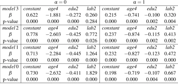
The final selected models include only the auxiliary variables appearing in Table 1. We have included three statistically significant variables that have a relevant meaning in the socio-economic sense. We have selected the variables age4(age group 50-65),
edu2(secondary education completed) andlab2(unemployed). Regression parameters and their corresponding p-values are also presented in Table 1 forα=0 andα=1.
By observing the signs of the regression parameters forα=0 (poverty proportion), we interpret that there is an inverse relation between poverty proportion and the cate-goriesage4and edu2of explanatory variables. That is, poverty incidence tends to be smaller in those domains with larger proportion of population in the subset defined by age between 50 and 64, and by secondary education level completed. On the other hand, poverty incidence tends to be larger in those domains with larger proportion of popu-lation in the subset defined bylab2, i.e. in the category of unemployed people. All the p-values are lower than 0.05 for all the considered auxiliary variables, except forlab2in model 3. By doing the same exercise with the signs of the regression parameters in the caseα=1 (poverty gap), we can give the same interpretations as before. Again all the p-values are lower than 0.05.
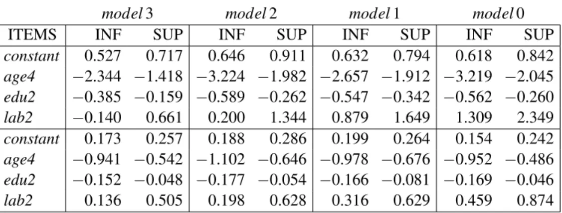
The asymptotic confidence intervals (CIs) for theβ’s at the 90% confidence level are presented in Table 2 (top) for α= 0 and in Table 2 (bottom) for α =1. The columns with labels INF and SUP contains the low and upper limits respectively. By
Table 1: β-parameters and p-values forα=0(left) andα=1(right).
α=0 α=1
model3 constant age4 edu2 lab2 constant age4 edu2 lab2
β 0.622 −1.881 −0.272 0.260 0.215 −0.741 −0.100 0.320
p-value 0.000 0.000 0.000 0.284 0.000 0.000 0.002 0.004
model2 constant age4 edu2 lab2 constant age4 edu2 lab2
β 0.778 −2.603 −0.425 0.772 0.237 −0.874 −0.115 0.413
p-value 0.000 0.000 0.000 0.026 0.000 0.000 0.002 0.002
model1 constant age4 edu2 lab2 constant age4 edu2 lab2
β 0.713 −2.284 −0.445 1.264 0.232 −0.827 −0.123 0.472
p-value 0.000 0.000 0.000 0.000 0.000 0.000 0.000 0.000
model0 constant age4 edu2 lab2 constant age4 edu2 lab2
β 0.730 −2.632 −0.411 1.829 0.198 −0.719 −0.107 0.667
Table 2: 90%confidence intervals forα=0(top) and forα=1(bottom).
model3 model2 model1 model0
ITEMS INF SUP INF SUP INF SUP INF SUP
constant 0.527 0.717 0.646 0.911 0.632 0.794 0.618 0.842 age4 −2.344 −1.418 −3.224 −1.982 −2.657 −1.912 −3.219 −2.045 edu2 −0.385 −0.159 −0.589 −0.262 −0.547 −0.342 −0.562 −0.260 lab2 −0.140 0.661 0.200 1.344 0.879 1.649 1.309 2.349 constant 0.173 0.257 0.188 0.286 0.199 0.264 0.154 0.242 age4 −0.941 −0.542 −1.102 −0.646 −0.978 −0.676 −0.952 −0.486 edu2 −0.152 −0.048 −0.177 −0.054 −0.166 −0.081 −0.169 −0.046 lab2 0.136 0.505 0.198 0.628 0.316 0.629 0.459 0.874
observing these confidence intervals, we conclude that all the regression parameters are significantly different from zero in both cases. The only exception islab2in model 3 for α=0.
Table 3 presents the CIs for the variance components at the 90% confidence level, under models 3-0, forα=0 andα=1. The columns with labels INF and SUP contains the low and upper limits respectively. The column with label 0∈CI contains T (true) if 0 belongs to the CI and F (false) otherwise. Concerning model 3, we observe that the CIs forρA−ρB andσA2−σ2Bcontain the 0. In the case ofα=0, the observed value of the
likelihood ratio statistics for testingH0:ρA=ρBisλ=0.5738 and the corresponding
p-value is 0.4487. In the case ofα=1, the observed value of the likelihood ratio statistics for testingH0:ρA=ρBisλ=3.8195 and the corresponding p-value is 0.0506. These
facts suggest that model 3 is not the model fitting best to data. Table 3: 90%confidence intervals for variances.
α=0 α=1
Model Parameter INF SUP 0∈CI INF SUP 0∈CI
3 σ2 A 0.0002 0.0008 F 0.0003 0.0005 F σ2 B 0.0005 0.0014 F 0.0002 0.0004 F σ2A−σ2B −0.0010 0.0001 T −0.0000 0.0003 T ρA 0.8662 0.9957 F 0.5416 0.7484 F ρB 0.8598 0.9344 F 0.6017 0.8843 F ρA−ρB −0.0409 0.1087 T −0.2734 0.0774 T 2 σ2A 0.0101 0.0154 F 0.0014 0.0019 F σ2 B 0.0023 0.0038 F 0.0004 0.0005 F σ2 A−σ2B 0.0070 0.0124 F 0.0009 0.0015 F ρ 0.4050 0.6108 F 0.3528 0.5756 F 1 σ2A 0.0025 0.0040 F 0.0004 0.0004 F σ2 B 0.0028 0.0045 F 0.0006 0.0007 F 0 σ2u 0.0025 0.0040 F 0.0004 0.0006 F
Table 4: Normalized Euclidean distances forα=0,1.
Model 3 Model 2 Model 1 Model 0
α Men Women Men Women Men Women Men Women
0 0.0194 0.0255 0.0083 0.0421 0.0285 0.0486 0.0648 0.0673 1 0.0115 0.0116 0.0121 0.0221 0.0188 0.0229 0.0290 0.0303
For models 2-0 Table 3 shows that the CIs forσ2
A,σ2Bandσ2udo not contain the origin
0 in any case, so the variances are significatively positive. Table 3 also presents the CIs for the difference of variancesσ2
A−σB2and the CIs forρunder model 2. The variances
σ2
Aandσ2Bcan be considered as different at the 90% confidence level and the correlation
parameterρ is significantly greater than zero in both cases (α=0 and α=1). In the caseα=0 the REML likelihood ratio statistic (LRS) for testingH0:σA2=σ2Btakes the
value 1210.06 and its corresponding p-value is 0.00. In the case ofα=1 the value of the REML LRS for testingH0:σ2A=σ2B is 1599.96 and the corresponding p-value is
0.00. In both cases we reject the null hypothesis of equality of variances. Therefore we can recommend model 2 for both poverty indicators.
Table 4 presents the normalized Euclidean distances between the direct and the EBLUPs estimates in both casesα=0 andα=1. We use the formula
D(y1,y2) = 1 M D
∑
d=1 md∑
t=1 (y1dt−y2dt)2 !1/2 .The obtained results are somehow expected. The models with more parameters present the lower normalized Euclidean distances. The extreme case would be a saturated model with as many parameters as observations, which has a perfect fit to data. As our target is explaining the data relationships, instead of looking for the best way of predicting the observedy-values, we do not modify our decision about model 3.
For being more confident about our decision of selecting model 2 as true generating model, we still give some diagnostics for models 0-2. At this stage, we drop out Model 3 from the selection procedure because of the hypotheses tested in Table 3.
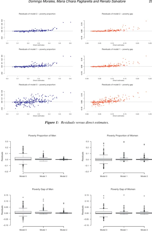
Residuals ˆedt =y¯dt−x¯Tdtβˆ −uˆdt of fitted models 2, 1 and 0 are plotted against the
observed values ¯ydt in the Figure 1 forα=0 (left) andα=1 (right). The dispersion
graph shows a great difference in the pattern of the plots, passing from the basic model 0 to the more complex model 2. In particular, residuals of model 2 present a more flattened shape than the ones of the other two models. Figure 2 presents the boxplots of residuals of models 0-2 and also shows that partitioned models 1 and 2 fit much better to the data than model 0. This conclusion coincides with the results appearing in Table 4, where Euclidean distances decrease as moving from model 0 to model 2. So we conclude that model 2 fits better to the direct estimates and therefore we can recommend it.
−0.2
0.0
0.1
0.2
0.3
Residuals of model 2 − poverty proportion
Direct estimates 0.0 0.1 0.2 0.3 0.4 0.5 0.6 −0.2 0.0 0.1 0.2 0.3 −0.2 0.0 0.1 0.2 0.3
Residuals of model 1 − poverty proportion
Direct estimates 0.0 0.1 0.2 0.3 0.4 0.5 0.6 −0.2 0.0 0.1 0.2 0.3 −0.2 0.0 0.1 0.2 0.3
Residuals of model 0 − poverty proportion
Direct estimates 0.0 0.1 0.2 0.3 0.4 0.5 0.6 −0.2 0.0 0.1 0.2 0.3 −0.10 0.00 0.10
Residuals of model 2 − poverty gap
Direct estimates 0.00 0.05 0.10 0.15 0.20 0.25 −0.10 0.00 0.10 −0.10 0.00 0.10
Residuals of model 1 − poverty gap
Direct estimates 0.00 0.05 0.10 0.15 0.20 0.25 −0.10 0.00 0.10 −0.10 0.00 0.10
Residuals of model 0 − poverty gap
Direct estimates
0.00 0.05 0.10 0.15 0.20 0.25
−0.10
0.00
0.10
Figure 1: Residuals versus direct estimates.
−0.2 −0.1 0.0 0.1 0.2 0.3
Poverty Proportion of Men
Residuals
Model 0 Model 1 Model 2
−0.10 −0.05 0.00 0.05 0.10 0.15
Poverty Gap of Men
Residuals
Model 0 Model 1 Model 2
−0.2 −0.1 0.0 0.1 0.2 0.3
Poverty Proportion of Women
Residuals
Model 0 Model 1 Model 2
−0.10 −0.05 0.00 0.05 0.10 0.15
Poverty Gap of Women
Residuals
Model 0 Model 1 Model 2
0.0 0.1 0.2 0.3 0.4 0.5 0.6
Estimated poverty proportion − MEN
Domains 1 6 10 15 19 24 28 33 37 42 46 51 0.0 0.1 0.2 0.3 0.4 0.5 0.6 Dir EBLUP 2 0.00 0.02 0.04 0.06 0.08 0.10
Root mean squared error of poverty proportion − MEN
Domains 1 6 10 15 19 24 28 33 37 42 46 51 0.00 0.02 0.04 0.06 0.08
0.10 Root MSE DirRoot MSE EBLUP 2
0.0 0.1 0.2 0.3 0.4 0.5 0.6
Estimated poverty proportion − WOMEN
Domains 1 6 10 15 19 24 28 33 37 42 46 51 0.0 0.1 0.2 0.3 0.4 0.5 0.6 Dir EBLUP 2 0.00 0.02 0.04 0.06 0.08 0.10
Root mean squared error of poverty proportion − WOMEN
Domains 1 6 10 15 19 24 28 33 37 42 46 51 0.00 0.02 0.04 0.06 0.08
0.10 Root MSE DirRoot MSE EBLUP 2
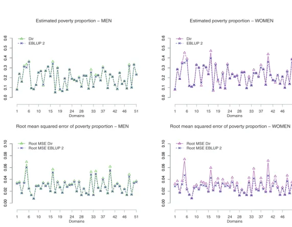
Figure 3: Estimates of poverty proportion (top) and squared root of their estimated MSEs (bottom) respectively for men (on the left) and women (on the right) in 2006.
The poverty proportion estimates, direct and EBLUP under model 2, are plotted in the Figure 3 with respect to the partition of the domains in men (left) and women (right). Figure 4 presents the same plots for the poverty gap. Concerning the root MSEs, these figures show that the EBLUPs under model 2 have lower MSE than the direct estimator. Therefore it is worthwhile using model-based estimators instead of the direct ones. As the estimated root MSE of the direct estimate of domain 42 is too large, Figure 3 does not plot the estimates of this domain and renumbers domains 43 to 52 as 42 to 51.
In the Figure 5 the Spanish provinces are plotted in 4 colored categories depending on the values of the EBLUP2 estimates in % of the poverty proportions and the gaps, i.e.
pd=100·Yˆ
eblup2
0;d,2006 andgd=100·Yˆ
eblup2
1;d,2006. We observe that the Spanish regions where
the proportion of the population under the poverty line is smallest are those situated in the north and east, like Catalu˜na, Arag´on, Navarra, Pa´ıs Vasco, Cantabria and Baleares. On the other hand the Spanish regions with higher poverty proportion are those situated in the centre-south, like Andaluc´ıa, Extremadura, Murcia, Castilla La Mancha, Canarias, Ceuta and Melilla. In an intermediate position we can find regions that are in the centre-north of Spain, like Galicia, La Rioja, Castilla Le´on, Asturias, Comunidad Valenciana and Madrid. If we investigate how far the annual net incomes of population under the
0.00
0.05
0.10
0.15
0.20
Estimated poverty gap − MEN
Domains 1 6 10 15 19 24 28 33 37 42 46 51 0.00 0.05 0.10 0.15 0.20 Dir EBLUP 2 0.00 0.01 0.02 0.03 0.04
Root mean squared error of poverty gap − MEN
Domains 1 6 10 15 19 24 28 33 37 42 46 51 0.00 0.01 0.02 0.03
0.04 Root MSE Dir Root MSE EBLUP 2
0.00
0.05
0.10
0.15
0.20
Estimated poverty gap − WOMEN
Domains 1 6 10 15 19 24 28 33 37 42 46 51 0.00 0.05 0.10 0.15 0.20 Dir EBLUP 2 0.00 0.01 0.02 0.03 0.04
Root mean squared error of poverty gap − WOMEN
Domains 1 6 10 15 19 24 28 33 37 42 46 51 0.00 0.01 0.02 0.03
0.04 Root MSE Dir Root MSE EBLUP 2
Figure 4: Estimates of poverty gap (top) and squared root of their estimated MSEs (bottom) respectively for men (on the left) and women (on the right) in 2006.
Table 5: Estimated poverty proportions (α=0) and RMSE’s in 2006.
Men Women
Province nd DIR EB2 RMSE⋆ RMSE2 nd DIR EB2 RMSE⋆ RMSE2 Soria 24 0.247 0.231 0.107 0.080 18 0.604 0.351 0.126 0.057 Segovia 60 0.234 0.231 0.061 0.055 60 0.438 0.360 0.071 0.046 Palencia 73 0.228 0.210 0.054 0.049 72 0.280 0.246 0.058 0.041 ´ Alava 98 0.083 0.079 0.034 0.033 100 0.079 0.085 0.032 0.028 Zamora 109 0.332 0.317 0.048 0.045 100 0.268 0.259 0.046 0.037 Huelva 124 0.192 0.191 0.036 0.035 124 0.253 0.235 0.040 0.033 Burgos 169 0.127 0.127 0.029 0.028 167 0.124 0.129 0.028 0.025 Albacete 173 0.237 0.239 0.035 0.034 193 0.285 0.283 0.037 0.031 Granada 189 0.301 0.297 0.036 0.035 229 0.342 0.326 0.034 0.030 Crdoba 221 0.312 0.311 0.034 0.032 233 0.307 0.303 0.033 0.029 C´aceres 261 0.252 0.252 0.030 0.029 303 0.332 0.328 0.031 0.027 Tenerife 373 0.263 0.262 0.027 0.027 397 0.286 0.283 0.026 0.024 Sevilla 473 0.209 0.209 0.020 0.020 492 0.228 0.227 0.020 0.019 Zaragoza 556 0.101 0.101 0.014 0.014 577 0.136 0.139 0.017 0.016 Barcelona 1367 0.083 0.084 0.008 0.008 1494 0.108 0.109 0.008 0.008
Table 6: Estimated poverty gapss (α=1) and RMSE’s for men in 2006.
Men Women
Province nd DIR EB2 RMSE⋆ RMSE2 nd DIR EB2 RMSE⋆ RMSE2 Soria 24 0.153 0.074 0.088 0.038 18 0.235 0.091 0.111 0.023 Segovia 60 0.070 0.069 0.021 0.019 61 0.123 0.102 0.025 0.017 Palencia 73 0.056 0.053 0.017 0.016 78 0.052 0.053 0.020 0.015 lava 98 0.025 0.024 0.010 0.010 87 0.107 0.101 0.018 0.014 Zamora 109 0.126 0.112 0.024 0.021 100 0.099 0.087 0.022 0.016 Huelva 124 0.105 0.091 0.027 0.023 124 0.091 0.077 0.021 0.015 Burgos 169 0.042 0.042 0.015 0.014 165 0.089 0.085 0.014 0.012 Albacete 173 0.096 0.095 0.017 0.016 181 0.053 0.051 0.012 0.010 Granada 189 0.135 0.124 0.020 0.018 194 0.112 0.109 0.017 0.014 Crdoba 221 0.082 0.083 0.011 0.011 230 0.114 0.106 0.015 0.012 Cceres 261 0.075 0.076 0.011 0.011 247 0.207 0.171 0.023 0.016 Tenerife 373 0.081 0.081 0.010 0.010 397 0.093 0.092 0.011 0.010 Sevilla 473 0.034 0.034 0.004 0.004 501 0.043 0.044 0.005 0.005 Zaragoza 556 0.043 0.043 0.009 0.009 605 0.027 0.028 0.005 0.005 Barcelona 1367 0.031 0.031 0.003 0.003 1494 0.036 0.036 0.004 0.004 pd<10 10<pd<20 20<pd<30 pd>30
Poverty Proportion − Men
pd<10 10<pd<20 20<pd<30 pd>30
Poverty Proportion − Women
gd<3 3<gd<6 6<gd<10 gd>10
Poverty Gap − Men
gd<3 3<gd<6 6<gd<10 gd>10
Poverty Gap − Women
Figure 5: EBLUP2 estimates of poverty proportions (top) and gaps (bottom) for men (left) and women (right) in 2006.
poverty linez2006 are fromz2006, we observe that in the Spanish regions situated in the
centre-north there exist a distance that is generally lower than the 6% ofz2006. However,
the cited distance is in general greater than 6% ofz2006in the centre-south.
Tables 5-6 present the direct and EBLUP estimates under model 2 of poverty proportions (α=0) and poverty gaps (α=1) for some Spanish provinces. The provinces were selected accordingly with the quantiles of the set of domain sample sizesnd. The
EBLUP estimates under the model 2 are labelled by EB2 and the direct estimates by
DIR. The squared root of MSEs are labelled by RMSE⋆for the direct estimator and by RMSE2for the EBLUP under the model 2 respectively. Numerical results are sorted by
sex. Regarding the reduction of the MSE when passing from direct to EBLUP estimates, we observe that model 2 performs better in domains with small sample size.
4. Discussion
As poverty indicators are nonlinear, unit-level model-based estimation approaches can-not always be used. However, their direct estimators are weighted sums that can be modelled by area-level models. Area-level models thus provide an easy-to-apply solu-tion. These idea motivates the introduction of partitioned temporal models that borrow strength from time. The use of information from past time instants, the greater avail-ability of auxiliary variables at the domain level and the possibility of introducing mod-elling differences by sex might compensate the loss of information when passing from unit-level models to area-level models. We thus considered four area-level linear mixed models and we applied the methodology to Spanish EU-SILC data.
We would also like to point out that model (1) and its particularizations have some features of interest, from a methodological point of view. It is somewhat different from the Rao-Yu model (Rao and Yu, 1994, and Rao, 2003), viewed as an extension of the Fay-Herriot area-level model in the case of time-correlated data. As we can note, the covariance matrix of the model does not contain the variance component connected with the random-effect at the domains, as clusters of time-correlated data. This fact permits to the random time-area effect to absorb completely the variation of the EBLUP due to the correlated observation, without considering any cluster-oriented random-effect components.
Another characteristic of main interest of the model (1), is that is a “partitioned” model. This means that different variance components in the covariance matrix of the random-area effects can accommodate different inputs of information, due to some relevant issues related to the specific levels of auxiliary variables. In the case of the application on the poverty indicators in Spain, the partitioning of the variance of the random-effect is significative for the gender-based class of survey domains. In fact, relevant differences in terms of the data in these classes of domains, as inputs in the fixed-effects regression, seems to drive at the same time to different variations in the related class of random-area effects.
The R programming language has been employed for doing all the computations in this paper. The deliverable D22 on software for small area estimation of the Euro-pean SAMPLE project (http://www.sample-project.eu/) gives a primary version of the employed R codes.
References
Das, K., Jiang, J. and Rao, J. N. K. (2004). Mean squared error of empirical predictor. Mean squared error of empirical predictor.The Annals of Statistics, 32, 818–840.
Datta, G. S. and Lahiri, P. (2000). A unified measure of uncertainty of estimated best linear unbiased predictors in small area estimation problems.Statistica Sinica, 10, 613–627.
Esteban, M. D., Morales, D., P´erez, A. and Santamar´ıa, L. (2012a). Small area estimation of poverty proportions under area-level time models.Computational Statistics and Data Analysis, 56, 2840– 2855.
Esteban, M. D., Morales, D., P´erez, A. and Santamar´ıa, L. (2012b). Two area-level time models for estimating small area poverty indicators.Journal of the Indian Society of Agricultural Statistics, 66, 75–89.
Foster, J., Greer, J. and Thorbecke, E. (1984). A class of decomposable poverty measures.Econometrica, 52, 761–766.
Ghosh, M. and Rao, J.N.K. (1994). Small area estimation: An appraisal.Statistical Science, 9, 55–93. Herrador, M., Esteban, M. D., Hobza, T. and Morales, D. (2011). A Fay-Herriot model with different
random effect variances.Communications in Statistics (Theory and Methods), 10, 785–797. Jiang, J. and Lahiri, P. (2006). Mixed model prediction and small area estimation.Test, 15, 1–96.
Marhuenda, Y., Molina, I. and Morales, D. (2013). Small area estimation with spatio-temporal Fay-Herriot models.Computational Statistics and Data Analysis, 58, 308–325.
Pfeffermann, D. (2002). Small area estimation-new developments and directions.International Statistical Review, 70, 125–143.
Pfeffermann, D. (2013). New important developments in small area estimation.Statistical Science, 28, 1– 134.
Prasad, N. G. N. and Rao, J. N. K. (1990). The estimation of the mean squared error of small-area estimators. Journal of the American Statistical Association, 85, 163–171.
Rao, J. N. K. (1999). Some recent advances in model-based small area estimation.Survey Methodology, 25, 175–186.
Rao, J. N. K. (2003).Small Area Estimation. John Wiley.
Rao, J. N. K. and Yu, M. (1994). Small area estimation by combining time series and cross-sectional data. Canadian Journal of Statistics, 22, 511–528.