Anomaly detection in GPS data based on visual analytics

(1)

c

(2)

ANOMALY DETECTION IN GPS DATA BASED ON VISUAL ANALYTICS

BY BINBIN LIAO

THESIS

Submitted in partial fulfillment of the requirements for the degree of Master of Science in Computer Science

in the Graduate College of the

University of Illinois at Urbana-Champaign, 2010

Urbana, Illinois Adviser:

(3)

ABSTRACT

Modern machine learning techniques provide robust approaches for data-driven modeling and critical information extraction, while human experts hold the advantage of possessing high-level intelligence and domain-specific expertise. We combine the power of the two for anomaly detection in GPS data by integrating them through a visualization and human-computer in-teraction interface.

In this thesis we introduce GPSvas (GPS Visual Analytics System), a system that detects anomalies in GPS data using the approach of visual analytics: a conditional random field (CRF) model is used as the machine learning component for anomaly detection in streaming GPS traces. A vi-sualization component and a user-friendly interaction interface are built to visualize the data stream, display significant analysis results (i.e., anomalies or uncertain predications) and hidden information extracted by the anomaly detection model, which enable human experts to observe the real-time data behavior and gain insights into the data flow. Human experts further provide guidance to the machine learning model through the interaction tools; the learning model is then incrementally improved through an active learning procedure.

(4)

(5)

ACKNOWLEDGMENTS

Thanks to Professor Yizhou Yu for his instruction and persistent help. Thanks to Tian Xia for discussion on the user interface design of the system. And special thanks to Wenjie for her constant support and love.

(6)

LIST OF TABLES

3.1 Feature set for anomaly detection in taxi GPS traces . . . 16 6.1 Summary of labeling accuracy. . . 32

(8)

LIST OF FIGURES

1.1 visual analytics approach illustration . . . 3 2.1 Overview of the system architecture . . . 6 2.2 A snapshot of the visual interface . . . 8 3.1 A graphical representation of a linear-chain CRF. For time

stept,Ytis a discrete hidden state, andXtis an observation data vector. The feature function set is defined over the

observation vector. . . 11 3.2 Illustration of data organization for CRF-based labeling.

A GPS data stream is divided into non-overlapping seg-ments, and the observation vectors within each segment are taken as an input sequence to the CRF model. Dt is the GPS raw data at time step t, and Xt is the derived observation vector. The output state sequence Y is the

anomaly detection result. . . 14 5.1 Example Hermite splines that approximate taxi

trajecto-ries given position samples (the red squares). . . 23 5.2 A visual representation of GPS traces. Taxi A is loaded

with passengers, and is highlighted with an orange stroke color to signal a potential anomaly. Taxi B is not loaded with passengers. Taxi C is selected by the mouse and high-lighted with a red stroke color. Nearby taxis of the selected taxi has a blue stroke color. The trajectory of the selected

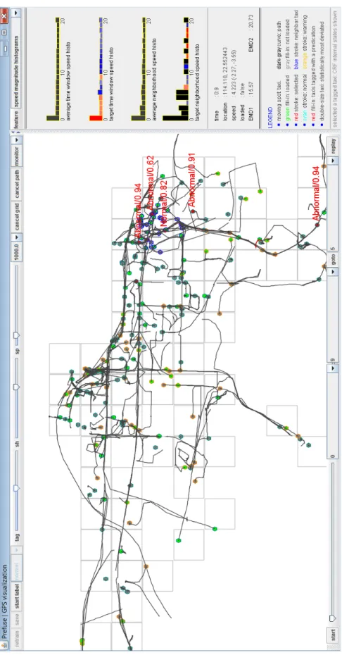
taxi is highlighted in red. . . 24 5.3 CRF internal states visualization. Top: the speed

his-togram for a time window, Bottom: the speed histogram for a spatial neighborhood. Each bucket in the histograms corresponds to a feature with the feature value represented by the height. Colors are used to reveal the degree of

(9)

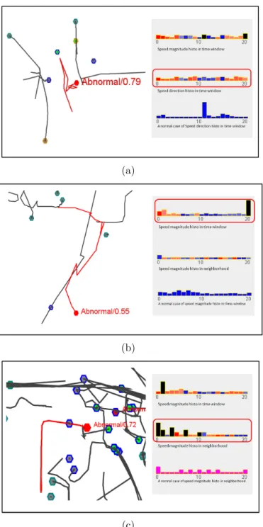
5.4 Representative abnormal cases and histograms. (a) An ab-normal case with an irregular pattern of driving directions. (b) An abnormal case involving high speed. (c) An ab-normal case with a crowded neighborhood (possible traffic jam). An identified critical factor is highlighted with a red

rectangle with rounded corners. . . 30 5.5 Information exploration at different scales. (a) A global

view of taxi trajectories with a superposed grid, (b) a zoom-in to a local area where anomalies occur, (c) further zoom-in to a finer scale to view the local taxi distribution

(10)

LIST OF ABBREVIATIONS

GPS Global Positioning System GPSvas GPS Visual Analytics System CRF Conditional Random Field MRF Markov Random Field HMM Hidden Markov Model

POS Part-Of-Speech

NER Name Entity Recognition

BFGS Broyden-Fletcher-Goldfarb-Shanno EMD Earth Mover’s Distance

(11)

LIST OF SYMBOLS

X Observation data variable for CRFs

Y Hidden states of CRFs

x Assignment of X y Assignment of Y

f Feature function vector of a CRF model

λ Weight vector of feature functions in a CRF model

S Candidate data sequence set

P(Y|X) Conditional probability of Y given X

C(y|x) Confidence estimation of predicationy given x

(12)

CHAPTER 1 INTRODUCTION

With the prevalence of the Global Positioning System (GPS), an increasing number of electronic devices and vehicles have been equipped with a GPS module for a variety of applications including navigation and location-based search. In addition to such conventional use, the GPS module can also be treated as a sensor that can regularly report the position and other status of the hosting vehicle or object. Such GPS traces provide very useful informa-tion regarding the temporal trajectory and the moving pattern of the host as well as indirect information regarding the surroundings of the host. In this paper, we focus on data analytics and anomaly detection of GPS traces of urban taxis.

There are three major objectives of such data analysis: 1) use taxi GPS traces to assist urban traffic monitoring because the speed of a taxi indirectly indicates the traffic condition on the street where the taxi is; 2) improve the safety of pedestrians and taxi passengers by monitoring and detecting reck-less behaviors of taxi drivers; 3) discover potential emergencies or abnormal situations associated with taxi drivers or passengers. There exist a few chal-lenges to achieve these objectives. First, we need to deal with a large number of simultaneous real-time data streams because there are typically a large number of taxis in an urban area; second, we need to efficiently analyze the temporal patterns of individual GPS traces as well as spatial distributions of these traces to report any abnormal traffic conditions or driving behaviors in

(13)

real time.

Manually analyzing hundreds of GPS traces is obviously unrealistic. On the other hand, a completely automatic approach would not be feasible either since abnormal situations need to be confirmed by human experts. There-fore, a visual analytics approach is taken to develop a semi-automatic system. There should exist both data analysis and visualization components in the system to support collaboration between machines and human analysts. The data analysis component is based on machine learning models. Fast auto-matic analysis is first performed by the data analysis component, which is also capable of providing the uncertainty of the analysis results. GPS traces along with analysis results are presented through the visualization engine. Human analysts can make use of the visualization in multiple different ways. Most of the time, the automatic analysis results are correct with high confi-dence. Therefore, human analysts can directly take the results provided by the machine. When a result is presented with high uncertainty, a human analyst can interact with our system to look at the details of the spatial and temporal patterns to correct the automatic analysis result. More impor-tantly, any user-provided analysis results can also be used as training data to improve the performance of the automatic data analysis component so that it can achieve a higher level of accuracy on future incoming data.

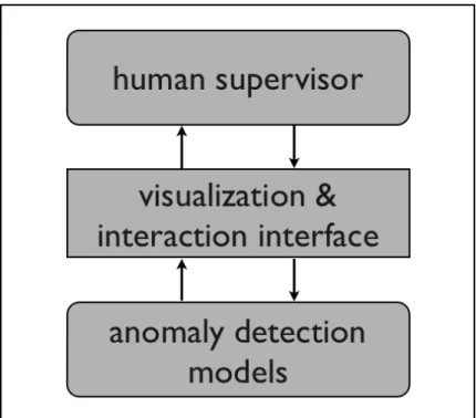
Our system harnesses the computing power of machine learning models and the high-level intelligence of human experts through a visualization en-gine and a human-computer interaction interface. Through the visualization and the interaction tools, human experts can choose to browse the most rele-vant information and provide guidance to the anomaly detection component. Figure 1.1 shows a high level view of these components. We use a state-of-the-art discriminative machine learning model, conditional random fields

(14)

Figure 1.1: visual analytics approach illustration

(CRFs), for anomaly detection. CRFs require supervised training. To mini-mize the amount of manual labeling, the performance of our CRF model is in-crementally improved through an active learning procedure. Active learning is a machine learning paradigm that the learner (machine model) selectively choose data items with a high prediction uncertainty as training set. This is because such data items are the most critical ones that can directly remove ambiguities in the machine model and effectively improve its performance.

The rest of this paper is organized as follows. In Section 2, we give an overview of our visual analytics system. In Section 3, we first give an overview of conditional random fields and then discuss in detail how to perform feature extraction in our CRF model for GPS anomaly detection. In Section 4, we first review the active learning approach, and then present the criteria we use to select candidate training data. In Section 5, we present our visualization component and the human-machine interface of our system. After that, we

(15)

demonstrate experimental results of our system on a set of GPS traces in Section 6. Related work and conclusions are given in Sections 7 and 8.

(16)

CHAPTER 2 OVERVIEW

GPS traces from hundreds of taxis within an urban area serve as the input to our system. Such data can be streamed to our system in real time. Data is automatically collected from every taxi once every few seconds. These collected data items form the trajectory of a taxi over time. A data item consists of 6 attributes: (ID, latitude, longitude, loaded, speed, time). ID

is the identification number of the taxi from which the data is collected.

latitude and longitude define the global location of the taxi. loaded is a boolean value indicating whether the taxi is loaded with passengers or not.

speed is simply the speed of the taxi at the time of collection. time is the time stamp of the GPS data item.

Our system consists of four major components: a machine model for anomaly detection, an active learning module, a visualization component, and a human-machine interaction interface. Figure 2.1 gives a overview of the system architecture.

The human-machine interaction interface forms the front-end of the sys-tem, while the back-end consists of the visualization engine, the active learn-ing module and an anomaly detection component based on the conditional random field (CRF) model. Since CRFs perform supervised classification, an initial CRF model with a reasonable classification accuracy needs to be trained in advance. The interaction interface supports three modes: basic mode, monitoring mode and tagging mode. A user can switch among these

(17)

Figure 2.1: Overview of the system architecture

three modes at any time. The basic mode only visualizes the raw GPS traces, and users can only perform basic exploration.

In the monitoring mode, the anomaly detection component is activated, and anomaly tags are shown dynamically on the screen. As shown in Figure 2.1, data passes through the visualization engine and the CRF model. At every time step, the CRF model predicts the status (normal or abnormal) of every taxi by analyzing the new incoming data together with previous data falling within a causal time window. The visualization engine takes the incoming GPS traces and the predicted labels from the CRF model to update the visualization on the screen. In addition, upon request from the user, the visualization engine can also show internal feature values used by the CRF model. Thus, human experts can not only verify the final analysis results from the CRF model but also gain additional insights by checking the evidences the CRF model uses to reach its conclusions.

(18)

In the tagging mode, the active learning module is activated. It uses the CRF model to mark data items whose labels are highly uncertain. High uncertainty indicates the current version of the CRF model has become inad-equate to label these data items automatically. Human experts are requested to manually label a representative subset of these marked items. Such labeled data can then be used to train an improved version of the CRF model.

The visual analytics approach taken in our system enables reliable detec-tion of anomalies with minimal user intervendetec-tion by effectively integrating automatic state-of-the-art machine learning techniques with human experts’ insights. Figure 2.2 shows a snapshot of the system.

(19)

(20)

CHAPTER 3 ANOMALY DETECTION BASED ON CRFS

3.1 Conditional Random Fields

Conditional random fields is a machine learning model for representing the conditional probability distribution of hidden states Ygiven observationsX. Intuitively, a conditional random field model builds the conditional proba-bility distributionP(Y|X) for determining the most probable labeling of ob-servation data. It was first introduced by Lafferty et al.[1] for text sequence segmentation and labeling, and has been successfully applied to many prob-lems in text processing, such as part-of-speech (POS) tagging [1] and name entity recognition (NER) [2], as well as problems in other fields, such as bioinformatics [3, 4] and computer vision [5].

Conditional random fields is a conditionally trained Markov random field (MRF) Y (hidden states) over observation data X. Different from genera-tive models, such as Hidden Markov Model (HMMs) [6], which model the joint probability P(Y,X), CRFs is a discriminative model that models the conditional probability P(Y|X). Two advantages are offered by taking a discriminative model over a generative model: (1) It takes the flexibility to include overlapping or long-range interaction features over the global input sequence X without any independence assumption to be made, since in a discriminative model we do not directly model the distribution of X, such as what a generative model does. (2) A discriminative model P(Y|X) can

(21)

be regarded as a generative model P(Y,X) = P(Y|X;θ)P(X;θ0) with the assumption that the estimations of θ and θ0 decouple [7], which means a discriminative model encompasses a broader set of probability distribution of (Y,X) and thus can fit the data better than a generative model, which assumes θ=θ0. In applications where the observationX is simple to model, a full generative model can offer certain advantage such as faster convergence given smaller set of training data [8]; however, in many real world applica-tions such as NLP, Bioinformatics, vision, or GPS traces, the observation data X tends to span a very large space and have complex internal interde-pendency structures. A generative model (e.g., HMMs) for such applications will either suffer from decrease in accuracy by making strong independence assumptions or loss of computational tractability by modeling the internal dependencies ofX. Given the two properties listed above, a conditional ran-dom fields model can often outperform over a generative model in the above mentioned applications.

In the remainder of the paper we limit our discussion of CRFs to linear-chain CRFs, which is the model we use for our GPS data anomaly detection.

3.2 Linear-Chain Conditional Random Fields

The state variables Y in a linear-chain conditional random field [1, 9] are restricted to form a chain. This assumption greatly simplifies the model complexity and yet is a very natural assumption in applications where the input X has a sequential form, such as text sequences for natural language processing problems or gene sequences for bioinformatics problems. Linear-chain condition random fields are well suited for modeling and classifying GPS data too because GPS data streams are essentially temporal signals

(22)

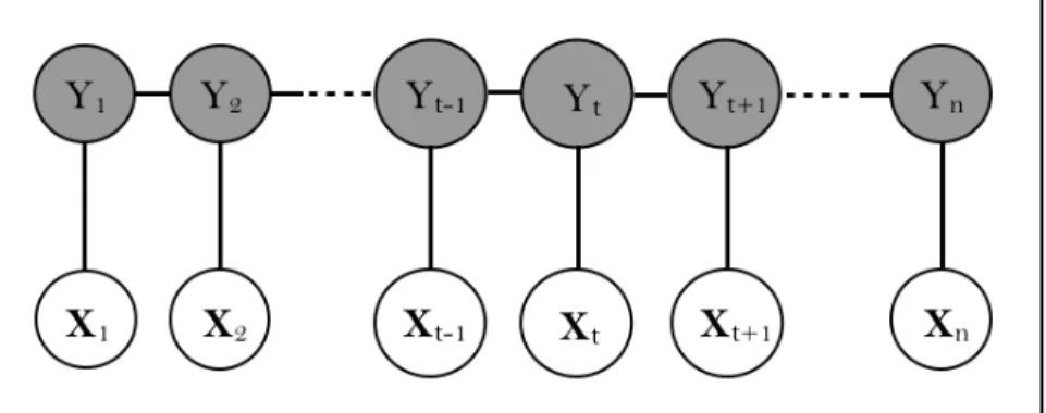
Figure 3.1: A graphical representation of a linear-chain CRF. For time step

t,Yt is a discrete hidden state, andXt is an observation data vector. The feature function set is defined over the observation vector.

and have a sequential nature.

The graphical representation of a linear-chain CRF is shown in Figure 3.1.

Yt is the hidden state variable for the node at positiont in the sequence, Xt is the observed data at positiont. Each state variableYtis only connected to the immediately preceding and following states. The probability distribution over the random variables (X,Y) is modeled after a Markov random field (undirected graphical model), as is shown in Figure 3.1. By the fundamental theorem of Markov random fields [10], which states that the joint probability of a MRF can be factorized into a product of potential functions over local cliques in the graph, the joint probability of the hidden state sequence y

conditioned on x can be written in the following form:

P(y|x) = 1 Z(x)exp{ N X t=1 K X k=1 λkfk(yt, yt−1,xt)} where Z(x) is the normalization item:

Z(x) =X y exp{ N X t=1 K X k=1 λkfk(yt, yt−1,xt)}

(23)

length of the input sequence and K is the size of the feature function set. Each fk is a feature function (potential function) that is defined over a local clique in the graph, and takes yt, yt−1 and items in the input observation

sequence as arguments. A weight vector λ = {λ1, ..., λk} is associated with the feature function set. The values in the weight vector determine how the feature functions contribute to the conditional probability computed by the model. The feature functions, {f1, ..., fk}, define a set of clique templates

for the CRF model: given an input sequence x, the graphical model for the sequence can be constructed by moving the feature templates over the sequence. Therefore, a CRF model is fully specified by the feature function set and the weight vector (f, λ).

Since a conditional random field is a supervised machine learning model, it needs to go through a supervised training stage before being used for new testing data.

• Training The training process computes the model parameters (the weight vector) according to labeled training data pairs {y,x}m _such that the log-likelihood

m X i=1 logP(y(i)|x(i)) = m X i=1 N X t=1 K X k=1 λkfk(y (i) t , y (i) t ,x (i) t )− m X i=1 logZ(x(i)) is maximized. The above objective function is convex so gradient-based optimization can guarantee to find the globally optimal solution. The state-of-the-art gradient ascent method for such an optimization problem is the limited-memory BFGS algorithm [11].

• Inference When a trained CRF model is applied to a novel input sequence, it tries to find the most likely hidden state assignmenty, i.e.,

(24)

the label sequence

y=argmax

y P(y|x)

for the unlabeled input sequence x. For linear-chain CRFs, this can be efficiently performed by dynamic programming (the Viterbi algo-rithm [6]) over the sequential hidden variables y.

For a detailed discussion on inference and training algorithms for CRFs, interested readers are referred to [9]. In the following section, we describe the task-specific details of our GPS anomaly detection component using linear-chain CRFs.

3.3 Feature Extraction

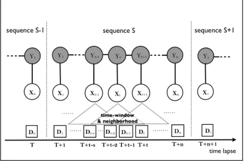
Given raw GPS data streams from taxi GPS devices, our anomaly detection component intends to automatically identify taxis with abnormal driving be-haviors. The value of hidden statesYis thus limited to{abnormal, normal}. The observation sequence X is derived from the raw GPS streams. Specif-ically, at each time step, incoming raw data items are preprocessed, and a new observation vectorXtis extracted for every taxi. The observation vector is derived from data with a time stamp inside a time window and a spatial location inside a neighborhood of the target taxi. A detailed description of the feature functions used in our CRF model is given in the following part of the section. We divide a GPS data stream into non-overlapping segments, and take the observation vectors within each segment as an input sequence to the CRF model. In our system, a segment typically includes 200 seconds of data. For each input sequence, the computed hidden states are used as the predicted labels of the taxi over a corresponding time interval. Figure 3.2

(25)

Figure 3.2: Illustration of data organization for CRF-based labeling. A GPS data stream is divided into non-overlapping segments, and the

observation vectors within each segment are taken as an input sequence to the CRF model. Dt is the GPS raw data at time step t, and Xt is the derived observation vector. The output state sequence Y is the anomaly detection result.

illustrates how the data is organized and processed in the CRF framework. To a large extent the performance of a CRF model is determined by the selection of the feature function set. In our GPS anomaly detection, the features at a time step are based on speed, time, location and passenger loading information. See the summarization of features in Table 3.1.

• speed: Speed is a primary source of cues that indicate driving behaviors. Instead of simply taking the speed of the target taxi at a single time step alone as a feature function, we rely on statistical properties, including his-tograms of the target taxi’s speed in a time window [T−s, T], whereT is the current time step, and histograms of the speed of taxis in a neighborhood of the target taxi at T. Speed is decomposed into magnitude and direction. Therefore there are four histograms in total, the histogram of speed magni-tude in a time window, the histogram of speed direction in a time window,

(26)

the histogram of speed magnitude in a spatial neighborhood, and the his-togram of speed direction in a spatial neighborhood. Each hishis-togram has 20 bins, and every bin of a histogram defines a feature function. Specifically, for a histogram of speed magnitude, the magnitude is discretized into 20 intervals, and each bin represents one interval. Similarly, for a histogram of speed direction, the direction is also discretized into 20 intervals, and each bin represents an angular interval of 18 degrees. The count (height) of a bin is the number of occurrences with the corresponding attribute interval. In addition to individual histograms, a mean histogram of each of the four types is also calculated over all taxis; for each taxi, the Earth Mover’s Dis-tance (EMD) [12] between its individual histogram and the corresponding mean histogram is taken as an additional feature function. These EMDs serve as a global measurement of how much an individual histogram deviates from the overall average.

•time: Time is a potential feature function in the CRF feature function set. In GPS traces, time is represented as seconds from the start of the day. Time is discretized into the following intervals: morning, morning rush hour, noon, afternoon, afternoon rush hour, night, late night. This allows the model to detect important relation between time of a day and abnormal driving trends from training data, and use it as a cue for predication.

• location: Location in the raw GPS data is expressed as (longitude, lati-tude) coordinates. We partition the target urban area into a rectangular grid (districts in the urban area), and let the feature selection procedure automat-ically discovers implicit relationships between districts and the occurrence of abnormal driving cases. Again, We use location feature to automatically detect implicit relations between city region and abnormal driving trends.

(27)

type feature description

speed magnitude histogram in a time window speed direction histogram in a time window

speed speed magnitude histogram of the taxis in the neighborhood speed direction histogram of the taxis in the neighborhood speed magnitude histogram difference from averaged histogram

speed direction histogram difference from averaged histogram

location longitude and latitude interval discretization

time time interval discretization

loaded boolean value indicating whether loaded with passengers

Table 3.1: Feature set for anomaly detection in taxi GPS traces •load: With the same idea from time and location, whether a taxi is loaded with passengers is also taken as a potential feature function.

Note that the above discussion describes all candidate feature functions for the CRF model. During the training stage, the feature selection procedure automatically chooses a subset of most relevant features as the actual feature function set in the CRF model.

3.4 Comparisons

The conditionally trained CRF model is called a discriminative model. For our application such a discriminative model is preferred overgenerative mod-els, which model the joint probability P(Y,X) of the hidden states and observations. The reason lies in that in our GPS anomaly detection task, the observation sequence X has a high degree of inter-dependency relation. Generative models such as Hidden Markov Models simply ignore the inter-dependencies among X to achieve computational tractability at the cost of performance; while more complicated generative models that take into ac-count the internal dependency structures of the input sequence X will suffer

(28)

from loss of computational tractability during training and inference. How-ever, by directly modeling the conditional probability P(Y|X), CRFs avoid modeling the internal structure of the observation X without suffering from loss of performance. Another advantage is, the feature functions in a dis-criminative model do not need to specify completely a state or observation, while in a generative model each local feature function must specify all pos-sible state or observation value enumerations. Given this property we could expect that a CRF model can be estimated with less training data. A CRF model is also preferred for GPS anomaly detection over simpler models such as a logistic regression or naive Bayes model in terms of performance. In a logistic regression or a naive Bayes model, it treats the labeling of each hid-den state as an isolated task given the local feature set, without considering the states of previous and next time slice. CRFs optimizes the overall label assignment over a sequence of observation by modeling both the local fea-ture set and the state transition probabilities. Thus we could expect CRFs to produce more smooth and reliable labeling results.

(29)

CHAPTER 4 ACTIVE LEARNING

Active learning is a general learning paradigm and many variations exist. The active learning scenario we have in the system is most related to pool-based active learning, where the learner proactively chooses a sample set of data items from a (usually very large) set of unlabeled data as the candidate training set to limit the amount of labeled data required for the learner to reach an acceptable level of accuracy [13, 14] or an increased level of general-ization [15,16]. Pool based active learning is a practical and effective learning method in many applications where unlabeled data is easily obtainable while manual labeling is expensive. This is exactly the case in our system. We have an unlimited amount of streaming data while manual labeling on such data is laborious. The success of an active learning procedure depends on the sample selection criteria. In the literature, many different criteria have been proposed including label uncertainty [16] and prediction variance [17].

In our system, we adapt the criteria proposed in [18] for CRF-related sam-ple selection. These criteria take into account samsam-pleuncertainty, representa-tiveness, anddiversity to choose non-redundant samples of high uncertainty as the training set. Among the three, uncertainty measures the level of confi-dence a CRF model labels a data sequence. Representativeness and diversity measure the similarity among samples. The active learning procedure first chooses a set of candidate samples with the highest uncertainty, and then uses the representativeness criterion to refine the candidate set by filtering

(30)

out redundant data items in the candidate set. In the last step, we use the diversity criterion to select from the candidate set the ones that have not yet been covered in the training set. In the following we discuss our adapted version of these sample selection criteria.

Uncertainty A conditional random field provides a natural confidence measurement of the prediction it makes. For a sequence x, the confidence (conditional probability) of labelyi ofxi P(yi|x) can be efficiently computed using the forward/backword algorithm [18]. The overall confidence C(y|x) of the label sequence ygiven input sequencexis defined to be the minimum confidence among all labels in the sequence, i.e., C(y|x) = miniP(yi|x). Given the definition of the confidence of a sample sequence x, the uncer-tainty measure is defined as

U ncertainty(x) = 1−C(y|x).

Representativeness For the subset of data sequences with high uncer-tainty S, a representativeness measure is defined over each sequence Si as following, Representativeness(Si) = 1 |S| −1 |S| X j=1,j6=i 1−Sim(Si,Sj),

where Sim(Si,Sj) is the similarity between two sequences. Given two se-quences Si =< pi1, ...pim > and Sj =< pj1, ...pjm > (pik is the k-th data item in sequence Si, m is the length of a sequence. Note that in our system all sequences are of the same length), Sim(Si,Sj) = _m1 Pm_k₌₁cos (pik, pjk) =

1

m

Pm

k=1

pik·pjk

kpikkkpjkk, which is the average pairwisecosine similarity over the en-tire sequences. A high representativeness value means that a sample sequence

(31)

is not similar to any other sequence in the candidate set. Note the the more complicated calculation of representativeness in a general context [18] has been simplified in our system because the sequences are of the same length.

We use the following empirical formula

L(Si) = 0.6U ncertainty(Si) + 0.4Representativeness(Si)

to choose a candidate training set whose combined score L(Si) exceeds a prescribed threshold.

Diversity Once the candidate set with the highest combined scores have been chosen, we use the diversity measure to remove items that are redundant with respect to data items that are already in the training set from the pre-vious iteration. Specifically, for each of the sequencesSi in the candidate set, we add it to our final training set if the similarity score between Si and any item currently in the training set is not greater than η = (1 +avgSim)/2, where avgSim is the average pairwise similarity among all sequences cur-rently in the training set.

(32)

CHAPTER 5 VISUALIZATION AND INTERACTION

Visualization and interaction play a critical role in our system. It connects the back-end machine learning components with human analysts who moni-tor and guide the system’s execution. Three major functionalities have been accommodated in the visualization and interaction components.

• The visualization engine displays taxi trajectories and their associated text annotations generated from the anomaly detection component. This provides a general impression of the traffic flow and individual driving behaviors, for example, possible traffic jam zones and aggressive passing behaviors, to the system user.

• In addition to the above basic visualization functionality, our system can also visualize the internal feature values that the CRF model relies on to automatically label a vehicle, i.e., the most critical features that vote for or against the decision on an anomaly detection label. This information helps analysts gain additional insights on the streamed GPS data.

• The human-computer interaction interface allows the user to select spe-cific information to explore and to provide guidance to the underlying machine learning models.

Note that these three functionalities are organized as integrated visualization and interaction components of the system. They coordinate with each other

(33)

for presenting data and information, and conveying human knowledge and guidance to the machine models. The following three subsections discuss these three functionalities respectively.

We use the Prefuse visualization toolkit [19] for our visualization task. Prefuse is an extensible software framework for developing interactive infor-mation visualization applications with a rich set of layout, aniinfor-mation and dis-tortion functionalities. It also supports separation (mapping) of data items from their visual representations through table, graph or tree data struc-tures, which makes data better organized and visual representations more easily manipulated.

5.1 Visualizing GPS Traces

The GPS traces of the taxis pass through the system as data streams. These data streams are scanned only once and kept in the system for a while be-fore being discarded. Visualization of such GPS traces includes updating the location of the taxis, displaying a partial trajectory of each taxi as well as vi-sually presenting other information that is available in the trace records, such as whether a taxi is loaded with passengers. We also base on the statistics of speed in a time window to highlight potential anomalies.

Taxi Trajectory According to the sampling rate of the GPS data, the actual position of each taxi is updated every 10-20 seconds. Directly con-necting these position updates with line segments would produce unnatural zigzagging trajectories. We use a Cardinal spline [20] to generate a plausi-ble trajectory given the position samples. Since the original GPS position samples are not sufficiently dense, to avoid unrealistic undulations in the

(34)

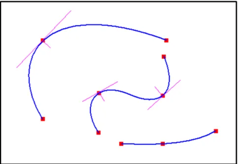
re-Figure 5.1: Example Hermite splines that approximate taxi trajectories given position samples (the red squares).

sulting spline, we choose an appropriate tension parameter for the Cardinal spline. Afterwards, the approximate position of the taxi at any time can be computed using this spline. This generates more continuous and natural trajectories of the taxis and produces smoother vehicle movements. Figure 5.1 shows some Hermite splines generated by interpolating a set of sample positions. The actual look of the taxi trajectories interpolated by Cardinal splines can be found in Figure 5.2. Note that the length of the partial tra-jectory of a taxi is determined by a fixed-size causal time window. A longer partial trajectory indicates a higher average speed in the time window.

Passenger Loading Each taxi is visually represented as a thick solid dot. Its filled color is used to indicate whether a taxi is loaded with passengers or not. Specifically, a green filled dot indicates the taxi is loaded, and black indicates the opposite.

(35)

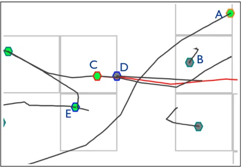
Figure 5.2: A visual representation of GPS traces. Taxi A is loaded with passengers, and is highlighted with an orange stroke color to signal a

potential anomaly. Taxi B is not loaded with passengers. Taxi C is selected by the mouse and highlighted with a red stroke color. Nearby taxis of the selected taxi has a blue stroke color. The trajectory of the selected taxi is highlighted in red.

Potential Anomalies In this part of visualization, we use a simple cue, speed magnitude, for detecting potential abnormal driving behaviors in an unsupervised way. Specifically, we calculate a histogram of speed for every taxi within a causal time window, and compute the Earth Mover’s Distance (EMD) between this histogram and the average histogram among all taxis. We also build a prior Gaussian model over the EMDs. Histograms with an EMD to the average histogram larger than twice the standard deviation of the Gaussian are considered potential anomalies. We use the stroke color of the solid dot to distinguish the potential anomalies from others. Orange is used for highlighting taxis with potential anomalies, and cyan is used for the others. In addition, at every time step, the taxi whose histogram has the largest EMD to the average histogram is highlighted by scaling its dot size by a factor of 3.

(36)

Such potential anomalies may be different from the anomalies labeled by the CRF model built using supervised training. These potential anomalies focus on fast moving taxis, which exhibit potentials to have true anomalous situations, while the anomalies labeled by the CRF model are more reliable because they are decided using a richer set of features with a sufficiently trained CRF model.

An example snapshot (part of the full screen) of trace visualization is shown in Figure 5.2.

5.2 Visualizing CRF Features

In a typical application, a CRF model is used as a black box: a user trains the model weights with a set of training data, and use the trained model to make predictions on unlabeled data afterwards. It is usually unclear to a user how the predictions are made. More specifically, what are the critical factors that contribute to the model’s output. In our visualization compo-nent, we developed a module that visualizes the internal information of the CRF model to illustrate how a decision is made inside the CRF model. The internal information includes the current state of features and their weights. Visualizing such information provides the possibility that if inappropriate weights are found in the CRF model, one could tune those weights in the right direction by adding specific labeled training data through the active learning procedure. To the best of our knowledge, this is the first attempt to visualize the internal states of CRF models.

A CRF model consists of two parts: the feature set, and the weights associated with the features. In practical applications, the feature set tends to be very large such that it would be impossible to gain understanding into

(37)

Figure 5.3: CRF internal states visualization. Top: the speed histogram for a time window, Bottom: the speed histogram for a spatial neighborhood. Each bucket in the histograms corresponds to a feature with the feature value represented by the height. Colors are used to reveal the degree of correlation (positive or negative) with the predicted label.

the model by directly displaying them in plain texts. In our visualization component, we use visual representations of the features and their weights instead. When a user selects a specific data item, the subset of features that is turned on for the specific data item are visualized, as well as the associated weights. For example, for a specific taxi at time step t, an ”on” feature could be ”the number of other nearby taxis whose speed is lower than 10 is between 5 and 10”. In the next time step, this feature would probably become ”the number of other nearby taxis whose speed is lower than 10 is less than 5”. From this example we see that for different taxis or different time steps, each feature takes potentially a different value. In our visualization scheme, a feature is represented by a rectangular bar, the height of which encodes its value (count), and the color of which encodes the weight associated with the feature. Positive weights are shown as red while negative

(38)

weights are shown as blue. A linear interpolation is used to obtain colors for intermediate weights. Figure 5.3 shows an example of the visualization of a feature set consisting of bins in the speed histograms. Representative abnormal cases and their histograms are shown in Figure 5.4.

5.3 Interaction Interface

Human-machine interaction is another indispensable part of our system. In our system, interaction is bi-directional: on one hand users explore the vi-sualized taxi partial trajectories and their associated text labels indicating whether any anomalies have been automatically detected; on the other hand, the underlying active learning module proactively selects items with highly uncertain labels and requests feedbacks from human experts. Human ex-perts give responses by manually providing labels to the requested items. Such labels are used for training an improved version of the CRF model.

To accommodate different types of user interaction described above, our system is designed to have three interaction modes: basic mode, monitor-ing mode and tagging mode. The basic mode only visualizes the raw GPS traces without any labels, and users can only perform basic exploration. In the monitoring mode, the anomaly detection component is activated, and anomaly tags are shown dynamically on the screen. Users can also choose to view the internal CRF states of the tagged data items. In the tagging mode, the active learning module is activated. Highly uncertain labels from the CRF model are highlighted, requesting for user input. CRF model train-ing with the newly labeled data is also activated in the taggtrain-ing mode. In the following we describe each of these three modes and their corresponding interactions.

(39)

Basic Mode Basic interactions in this mode includes: (a) zoom-in/zoom-out, which is controlled by mouse scroll, (b) dragging, which translates the center of the view port on the 2D plane by direct mouse dragging, (c) taxi selection, which highlights the selected taxi whose detailed information is also displayed on screen, (d) replay, which goes back in time to show the data that has just passed by. This allows users to check important scenarios of the traffic when necessary. There are a few other interaction operations such as pause/resume, change neighborhood radius for extracting the neighborhood features, information filtering to control the set of visual items (trajectories, grid) to be rendered on screen, and change the size of the fonts and taxi items, etc. Note that all the operations in this mode are available in the other modes as well. Figure 5.5 shows the zoom-in affects with various visualization settings at different levels.

Monitoring Mode The extra computation in the monitoring mode is run-ning the anomaly detection component. Feature sequences of the taxis are periodically fed to the CRF model, which returns automatically tagged re-sults to the visualization engine, which adds text annotations to the taxis if being labeled as anomalies. The anomalies are highlighted by setting the filled color to red. The annotation for a detected anomaly consists of a text string and an associated confidence value. In this mode, internal CRF fea-ture values and weights that contribute to a labeling result can be visualized when the analyst selects the specific taxi which the labeling result is associ-ated with.

Tagging Mode Different from the monitoring mode, the tagging mode is not for monitoring the anomalous cases but for collecting manually labeled

(40)

results used in active learning. In the tagging mode, the active learning mod-ule selects representative taxis whose predicted labels are highly uncertain and send them to the visualization engine. The visualization engine shows such predicted labels (”normal” or ”abnormal”) and their uncertainty values together with the taxis. Human experts can select any of these items and assign it a manual label to either confirm or correct the predicted label. The number of mouse clicks is minimized in such a way that clicks are only re-quired when the label needs to be flipped. At the end of manual tagging, the user can trigger the system to train an improved version of the CRF model using the manually labeled data. Once the training concludes, our system switches to the updated CRF model.

(41)

(a)

(b)

(c)

Figure 5.4: Representative abnormal cases and histograms. (a) An abnormal case with an irregular pattern of driving directions. (b) An abnormal case involving high speed. (c) An abnormal case with a crowded neighborhood (possible traffic jam). An identified critical factor is

(42)

(a)

(b) (c)

Figure 5.5: Information exploration at different scales. (a) A global view of taxi trajectories with a superposed grid, (b) a zoom-in to a local area where anomalies occur, (c) further zoom-in to a finer scale to view the local taxi distribution (trajectories of unselected taxis are hidden).

(43)

CHAPTER 6 ANOMALY DETECTION PERFORMANCE

We have tested the anomaly detection performance of our GPS visual analyt-ics system on an Intel i7-860 2.8GHz Quad Core processor. In this following we discuss the experimental setup and results on anomaly detection using CRFs.

Query by Committee We use the query-by-committee strategy instead of a single model to improve the robustness of anomaly detection. Specifi-cally, Five separate CRF models are initially trained using different sets of training sequences. Given a new sequence, each of the five models makes an independent prediction and the one with the highest confidence level is chosen as the final result. In other words, we choose the prediction result by the committee member who has the highest confidence in its decision.

train 1 2 3 4 5 AVG QBC baseline 0.62 0.72 0.77 0.61 0.66 0.67 0.66 0.28 0.28 0.36 0.40 0.32 0.32 0.44 train1 0.83 0.73 0.87 0.79 0.77 0.80 0.88 0.44 0.28 0.48 0.32 0.48 0.40 0.40 train2 0.83 0.78 0.82 0.82 0.82 0.81 0.90 0.48 0.32 0.48 0.40 0.44 0.42 0.52

Table 6.1: Summary of labeling accuracy.

Accuracy Table 6.1 summarizes the prediction accuracy of the individual models, averaged result and the query-by-committee model. The first line of

(44)

each compound row is the item accuracy and the second line is thesequence accuracy. Sequence accuracy is the ratio of testing sequences on which the predication label sequence matches the labeled sequence in every position. Item accuracy measures the testing accuracy by breaking each test sequence into separate items (labels at individual time slices).

Prediction accuracy is shown for three different versions of each model, the initial version trained with relatively little training data, and two versions trained after the first and second round of active learning. It is obvious that active learning steadily improves labeling accuracy over iterations. Given the prediction accuracy of the five individual CRF models, their average (ex-pected) accuracy and the final prediction accuracy of the query-by-committee model, we confirm that the query-by-committee strategy can in general im-prove prediction accuracy (compare the last two columns of Table 6.1), and can potentially achieve performance better than any of the individual mod-els.

(45)

CHAPTER 7 RELATED WORK

GPS signal indicates the temporally changing location of the GPS device wearer. Many techniques and systems have been developed to visualize GPS or trajectory data in a 2D or 3D space. A system is introduced in [21] for visualizing real-time multi-user GPS data from the Internet in a 3D VRML model. GPSVisualizer, Google Earth, Yabadu Maps, GPS-Track-Analyse.NET and FUGAWI Global Navigator are examples of online sys-tems that support the visualization of GPS data in various applications. The prevalence of GPS devices and wearable computing devices make wear-able computing [22, 23] a new emerging field of research. A recent technique for visualizing aircraft trajectories has also been presented in [24].

Our system integrates GPS data visualization with anomaly detection us-ing conditional random field models. This type of application has not yet been found in the visual analytics literature. In machine learning, however, there is an increasing popularity in information retrieval [25], behavior clas-sification or human activity understanding [26, 27] based on mobile sensor data, i.e., GPS data. In [25], the authors use hierarchically constructed conditional random fields to model human activities and extract significant locations in a map from GPS traces. Although [25] uses a similar type of data and learning model as we do, the difference lies in that their goal is to discover important patterns and locations in human activities while our goal is to perform anomaly detection in taxi driving behaviors. They try to

(46)

develop a completely automatic method while our system is semi-automatic and human-computer interaction is essential. We adopt a visual analytics approach to integrate human expertise and achieve a good performance. An-other difference is that the data in [25] has simpler patterns than our taxi GPS traces since the everyday activities of a person is more predictable than taxi moving patterns.

(47)

CHAPTER 8 CONCLUSIONS AND FUTURE WORK

In this thesis, we have introduced a visual analytics system for anomaly de-tection in urban taxi GPS data streams, and demonstrated that such an approach effectively integrates the power of machine learning models with human intelligence. Human understanding to the data and machine perfor-mance on anomaly labeling are mutually enhanced. In the system, we applied the conditional random field model to anomaly detection in GPS data and proposed a feature selection method, which is shown effective for the task by our experimental results. Active learning is used for minimizing the data labeling effort, providing a solution to incremental model improvement and allowing the model to adapt to the latest data as time involves. For stream-ing data, such an active learnstream-ing methodology is more adaptive compared with a passive learning one. Visualization and user interaction have been designed to selectively display the information according to users’ demand. In particular, we took effort to visualize the internal features and weights of a CRF model, which reveals critical internal mechanisms of such models that have been previously used as a black box.

There exist a few directions for future work. From the user’s perspective, more interaction tools and visualization affects can be developed for better information exploring to enhance human experts’ understanding to the data, for example, to support multi-window that shows information from different scales or views, or adding an external map as background to the visualization.

(48)

From the learning model’s perspective, one possible direction is to increase the number of hidden states, such as driving skill level and regional traffic status, in the CRF model, given that GPS traces provide relevant information as a type of sensor data. Another potential direction for future work is to extend the linear-chain CRF model to more complex models. For example, a hierarchical hidden Markov model [28] allows hidden states to be defined at different levels of granularity to model a hierarchical structure, or a semi-CRF model [29], which models hidden state transitions as a semi-Markov chain. Both models have a higher computational complexity, but with careful model design, we expect better performance in label prediction.

(49)

REFERENCES

[1] J. Lafferty, A. McCallum, and F. Pereira, “Conditional random fields: Probabilistic models for segmenting and labeling sequence data,” in Pro-ceedings of the International Conference on Machine Learning (ICML-2001), 2001.

[2] A. McCallum and W. Li, “Early results for named entity recognition with conditional random fields, feature induction and web-enhanced lex-icons,” in Proceedings of The Seventh Conference on Natural Language Learning (CoNLL-2003), 2003.

[3] Y. Liu, J. Carbonell, P. Weigele, and V. Gopalakrishnan, “Segmentation conditional random fields (scrfs): A new approach for protein fold recog-nition,” inACM International conference on Research in Computational Molecular Biology (RECOMB05), 2005.

[4] K. Sato and Y. Sakakibara, “Rna secondary structure alignment with conditional random fields,” in Bioinformatics, 2005, pp. 237–242. [5] S. Kumar and M. Hebert, “Discriminative fields for modeling spatial

dependencies in natural images,” in Advances in Neural Information Processing Systems 16. MIT Press, Combridge, MA, 2003.

[6] L. Rabiner, “A tutorial on hidden markov models and selected applica-tions in speech recognition,” in Proceedings of The IEEE, vol. 77, 1989. [7] T. Minka, “Discriminative models, not discriminative training,” in

Mi-crosoft Research Technical Report, 2005.

[8] A. Ng and M. Jordan, “On discriminative vs. generative classifiers: A comparison of logistic regression and naive bayes,” inAdvances in Neural Information Processing Systems 14, 2001, pp. 841–848.

[9] C. Sutton and A. McCallum, “An introduction to conditional random fields for relational learning,” in Introduction to statistical relational learning, chapter 4. MIT Press, Combridge, MA, 2007.

[10] J. M. Hammersley and P. Clifford, “Markov fields on finite graphs and lattices,” in unpublished manuscript, 1971.

(50)

[11] D. C. Liu and J. Nocedal, “On the limited memory bfgs method for large scale optimization,” in Mathematical Programming 45, 1989, pp. 503–528.

[12] E. Levina and P. Bickel, “The earthmovers distance is the mallows dis-tance: Some insights from statistics,” in Proceedings of International Conference on Computer Vision, 2001, pp. 251–256.

[13] M. Sassano, “An empirical study of active learning with support vec-tor machines for japanese word segmentation,” in Proceedings of the 40th Annual Meeting of the Association for Computational Linguistics (ACL), 2002.

[14] A. Finn and N. Kushmerick, “Active learning selection strategies for information extraction,” in ECML-03 Workshop on Adaptive Text Ex-traction and Mining, 2003.

[15] D. Cohn, L. Atlas, and R. Ladner, “Improving generalization with active learning,” in Machine Laerning, vol. 15, 1992, pp. 201–221.

[16] G. Schohn and D. Cohn, “Less is more: Active learning with support vector machines,” in Proceedings of the 17th International Conference on Machine Learning, 2000.

[17] Y. Freund, H. S. Seung, E. Shamir, and N. Tishby, “Selective sampling using the query by committee algorithm,” in Machine Learning, 1997, pp. 133–168.

[18] C. T. Symons, N. F. Samatova, R. Krishnamurthy, B. H. Park, T. Umar, D. Buttler, T. Critchlow, and D. Hysom, “Multi-criterion active learning in conditional random fields,” in Proceedings of the 18th IEEE Interna-tional Conference on Tools with Artificial Intelligence (ICTAI’06), 2006. [19] J. Heer, S. K. Card, and J. A. Landay, “prefuse: a toolkit for inter-active information visualization,” in Proceedings of Computer Human Interaction, 2005, pp. 421–430.

[20] I. J. Schoenberg, Cardinal Spline Interpolation. Society for Industrial Mathematics, 1987.

[21] I. Rakkolainen, S. Pulkkinen, and A. Heinonen, “Visualizing real-time gps data with internet’s vrml worlds,” inProceedings of the 6th ACM in-ternational symposium on Advances in geographic information systems, 1998, pp. 52–56.

[22] M. Billinghurst, S. Weghorst, and T. Furness, “Wearable computing for three dimensional cdcw,” inProceedings of the International Symposium on Wearable Computing, 1997.

(51)

[23] S. Feiner, B. MacIntyre, T. Hllerer, and A. Webster, “A touring ma-chine: Prototyping 3d mobile augmented reality systems for exploring the urban environment,” in Personal and Ubiquitous Computing, 2006, pp. 208–217.

[24] C. Hurter, B. Tissoires, and S. Conversy, “Fromdady: Spreading aircraft trajectories across views to support iterative queries,” in IEEE Trans-actions on Visualization and Computer Graphics, 2009, pp. 1017–1024. [25] L. Liao, D. Fox, and H. Kautz, “Extracting places and activities from gps traces using hierarchical conditional random fields,” International Journal of Robotics Research, vol. 26, 2007.

[26] B. L. Harrison, S. Consolvo, and T. Choudhury, “Using multi-modal sensing for human activity modeling in the real world,” in Handbook of Ambient Intelligence and Smart Environments, 2009.

[27] H. Lu, W. Pan, N. D. Lane, T. Choudhury, and A. T. Campbell, “Sound-sense: Scalable sound sensing for people-centric applications on mobile phones,” in The International Conference on Mobile Systems, Applica-tions, and Services, 2009.

[28] S. Fine and Y. Singer, “The hierarchical hidden markov model: Anal-ysis and applications,” in MACHINE LEARNING. Kluwer Academic Publishers, Boston, 1998, pp. 41–62.

[29] S. Sarawagi and W. W. Cohen, “Semi-markov conditional random fields for information extraction,” in In Advances in Neural Information Pro-cessing Systems 17, 2004, pp. 1185–1192.