WORKING PAPER SERIES
Predictable Dynamics in the S&P 500 Index
Options Implied Volatility Surface
Silvia Gonçalves
and
Massimo Guidolin
Working Paper 2005-010A
http://research.stlouisfed.org/wp/2005/2005-010.pdf
January 2005
FEDERAL RESERVE BANK OF ST. LOUIS
Research Division
411 Locust Street
St. Louis, MO 63102
______________________________________________________________________________________ The views expressed are those of the individual authors and do not necessarily reflect official positions of the Federal Reserve Bank of St. Louis, the Federal Reserve System, or the Board of Governors.
Federal Reserve Bank of St. Louis Working Papers are preliminary materials circulated to stimulate discussion and critical comment. References in publications to Federal Reserve Bank of St. Louis Working Papers (other than an acknowledgment that the writer has had access to unpublished material) should be cleared with the author or authors.
Predictable Dynamics in the S&P 500 Index Options
Implied Volatility Surface
∗
S´
õlvia Gon¸calves
†CIREQ, CIRANO and D´epartement de Sciences ´
Economiques, Universit´
e de Montr´
eal
Massimo Guidolin
University of Virginia
‡October 15, 2004
Abstract
One key stylized fact in the empirical option pricing literature is the existence of an implied volatility surface (IVS). The usual approach consists of Þtting a linear model linking the implied volatility to the time to maturity and the moneyness, for each cross section of options data. How-ever, recent empirical evidence suggests that the parameters characterizing the IVS change over time. In this paper we study whether the resulting predictability patterns in the IVS coefficients may be exploited in practice. We propose a two-stage approach to modeling and forecasting the S&P 500 index options IVS. In theÞrst stage we model the surface along the cross-sectional moneyness and time-to-maturity dimensions, similarly to Dumas et al. (1998). In the second-stage we model the dynamics of the cross-sectionalÞrst-stage implied volatility surface coefficients by means of vector autoregression models. WeÞnd that not only the S&P 500 implied volatility surface can be success-fully modeled, but also that its movements over time are highly predictable in a statistical sense. We then examine the economic signiÞcance of this statistical predictability with mixed Þndings. Whereas proÞtable delta-hedged positions can be set up that exploit the dynamics captured by the model under moderate transaction costs and when trading rules are selective in terms of expected gains from the trades, most of this proÞtability disappears when we increase the level of transaction costs and trade multiple contracts offwide segments of the IVS. This suggests that predictability of the time-varying S&P 500 implied volatility surface may be not inconsistent with market efficiency.
JEL code: G12, G13.
∗We would like to thank Peter Christoffersen, Steven Clark, Patrick Dennis, Kris Jacobs, and seminar participants at the 2003 Midwest Finance Association meetings for helpful comments. We are especially grateful to an anonymous referee, Ren´e Garcia, Rob Engle and Hal White for their comments and suggestions at various stages of this project, which greatly improved the paper.
†C.P. 6128, succ. Centre-Ville, Montr´eal, QC, H3C 3J7, Canada. Tel: (514) 343 6556. Email:
[email protected]. Gon¸calves acknowledgesÞnancial support from IFM2.
‡Correspondence to: Massimo Guidolin, Department of Economics, University of Virginia, Charlottesville - 114 Rouss
1. Introduction
Volatilities implicit in observed option prices are often used to gain information on expected market volatility (see e.g. Poterba and Summers 1986; Jorion 1995; Christensen and Prabhala 1998, and Fleming 1998). Therefore accurate forecasts of implied volatilities may be valuable in many situations. For instance, in derivative pricing applications, volatility characterizes the beliefs of market participants and hence is intimately related to the fundamental pricing measure. Implied volatilities are commonly used by practitioners for option pricing purposes and risk management.
Implied volatilities are typically found by Þrst equating observed option prices to Black-Scholes (1973, henceforth BS) theoretical prices and then solving for the unknown volatility parameter, given data on the option contracts and the underlying asset prices. Contrary to the BS assumption of constant volatility, implied volatilities tend to systematically vary with the options strike price and date of expiration, giving rise to animplied volatility surface (IVS). For instance, Canina and Figlewski (1989) and Rubinstein (1994) show that when plotted against moneyness (the ratio between strike price and the underlying spot price), implied volatilities describe either an asymmetric smile or a smirk. Campa and Chang (1995) show that implied volatilities are a function of time to expiration. Furthermore, the IVS is known to dynamically change over time, in response to news affecting investors’ beliefs and portfolios.
Practitioners have long tried to exploit the predictability in the IVS. The usual approach consists ofÞtting linear models linking implied volatility to time to maturity and moneyness, for each available cross-section of option contracts at a point in time. The empirical evidence suggests that the estimated parameters of such models are highly unstable over time. For instance, Dumas, Fleming and Whaley (1998) (henceforth DFW) propose a model in which implied volatilities are a function of the strike price and time to maturity. They observe that the coefficients estimated on weekly cross-sections of S&P 500 option prices are highly unstable. Christoffersen and Jacobs (2004) report identical results. Similarly, Heston and Nandi (2000) estimate a moving window nonlinear GARCH(1,1) and show that some of the coefficients are unstable. To explain the superior performance of their GARCH-pricing model, Heston and Nandi (2000) stress the ability of the GARCH framework to exploit the information on path-dependency in volatility contained in the spot S&P 500 index. Thus, time variation of the S&P 500 IVS matters for option pricing purposes.
In this paper we propose a modeling approach for the time series properties of the S&P 500 index options implied volatility surface. Our approach delivers easy-to-compute forecasts of implied volatilities for any strike price or maturity level. This is in contrast to the existing literature which has focused on either modeling the cross-section of the implied volatilities, ignoring the time series dimension, or on modeling the time series properties of an arbitrarily chosen point on the IVS, i.e. the volatility implicit in contracts with a given moneyness and/or time-to expiration. To the best of our knowledge, we are theÞrst to jointly model the cross-sectional features and the dynamics of the IVS for stock index options.
We ask the following questions: Given the evidence of time variation in the IVS, is there any gain from explicitly modeling its time series properties? In particular, can such an effort improve our ability to forecast volatility and hence option prices? To answer these questions, we combine
a cross-sectional approach to Þtting the IVS similar to DFW (1998) with the application of vector autoregression (VAR) models to the (multivariate) time series of estimated cross-sectional coefficients. Therefore, our approach is a simple extension of the DFW approach where modeling occurs in two distinct stages. In aÞrst stage, weÞt daily, cross-sectional models that describe implied volatilities as a function of moneyeness and time-to-maturity. Consistently with the previous literature, we report evidence of structure in the S&P 500 IVS and Þnd that a simple model linear in the coefficients and nonlinear in moneyness and time to maturity achieves an excellent Þt. The documented instability of the estimated cross-sectional coefficients motivates our second step: we Þt time series models of a VAR-type to capture the presence of time variation in the Þrst-stage estimated coefficients. We Þnd that the Þt provided by this class of models is remarkable and describes a law of motion for the IVS which conforms to a number of stylized facts.
To assess the performance of the proposed IVS modeling approach, we use both statistical and economic criteria. First, we study its ability to correctly predict the level and the direction of change of one-day-ahead implied volatility. We Þnd that our models achieve good accuracy, both in absolute terms and relatively to a few natural benchmarks, such as random walks for implied volatilities and Heston and Nandi’s (2000) NGARCH(1,1). Second, we evaluate the ability of our forecasts to support portfolio decisions. WeÞnd that the performance of our two-stage, dynamic IVS models at predicting one-step-ahead option prices is satisfactory. We then simulate out-of-sample delta-hedged trading strategies based upon deviations of volatilities implicit in observed option prices from model-based predicted volatilities with a constant,Þxed investment of $1,000 per day. The simulated strategies that rely on two-stage IVS models generate positive and statistically signiÞcant out-of sample returns when low-to-moderate transaction costs are imputed on all traded (option and stock) contracts. These proÞts are abnormal as signalled by Sharpe ratios in excess of benchmarks such as buying and holding the S&P 500 index, i.e. they are hardly rationalizable in the light of the risk absorbed. Importantly, ourÞnding of abnormal proÞtability appears to be fairly robust to the adoption of performance measures that take into account non-normalities of the empirical distribution of proÞts and to imputing transaction costs that account for the presence of bid-ask spreads. In particular, our approach is most accurate (hence proÞtable) on speciÞc segments of the IVS, mainly out-of-the-money and short- to medium-term contracts.
These results turn mixed when higher transaction costs and/or trading strategies that imply trades on large numbers of contracts along the entire IVS are employed in calculating proÞts. We conclude that predictability in the structure of the S&P 500 IVS is strong in statistical terms and ought to be taken into account to improve both volatility forecasting and portfolio decisions. On the other hand, such predictability patterns hardly represent outright rejections of the tenant that deep and sophisticated capital markets such as the S&P 500 index options market are informationally efficient. In particular, even whenÞlters are applied to make our trading rules rather selective in terms of the ex-ante expected proÞts per trade, we Þnd that as soon as transaction costs are raised to the levels that are likely to be faced by small (retail) speculators, all proÞts disappear.
The option pricing literature has devoted many efforts to propose pricing models consistent with the stylized facts derived in the empirical literature, of which the implied volatility surface is probably
the best known example. Models featuring stochastic volatility, jumps in returns and volatility, and the existence of leverage effects (i.e. a non-zero covariance between returns and volatility) are popular approaches (see Garcia, Ghysels and Renault (2003) for a review of the literature). More recently, several papers have proposed models relying on a general equilibrium framework to investigate the economics of these stylized facts.1 For instance, David and Veronesi (2002) propose a dynamic asset pricing model in which the drift of the dividend growth rate follows a regime switching process. In-vestors’ uncertainty about the current state of the economy endogenously creates stochastic volatility and leverage, thus giving rise to an implied volatility surface. Because investors’ uncertainty evolves over time and is persistent, this model induces predictability in the implied volatility surface. Similarly, Guidolin and Timmermann (2003) propose a general equilibrium model where dividends evolve on a binomial lattice. Investors learning is found to generate asymmetric skews and systematic patterns in the implied volatility surface. The changing beliefs of investors within a rational learning scheme imply dynamic restrictions on how the implied volatility surface evolves over time. Finally, in Gar-cia, Luger and Renault’s (2003) utility-based option pricing model, investors learn about the drift and volatility regime of the joint process describing returns and the stochastic discount factor, modeled as a bivariate regime switching model. Under their assumptions, the implied volatility surface depends on an unobservable latent variable characterizing the regime of the economy. Persistence of the process describing this latent variable implies predictability of the implied volatility surface. These models are examples of equilibrium-based models that generate time varying implied volatility patterns consistent with those observed in the data. We view our approach as a reduced form approach to model the time variation in the implied volatility surface that could have been generated by any of these models. As is often the case in forecasting, a simple reduced form approach as ours is able to efficiently exploit the predictability generated by more sophisticated models.
A few existing papers are closely related to ours. Harvey and Whaley (1992) study the time variation in volatility implied by the S&P 100 index option prices for short-term, nearest at-the-money contracts. They test the hypothesis that volatility changes are unpredictable based on regressions of the changes in implied volatility on information variables that include day-of-the-week dummy variables, lagged implied volatilities, interest rate measures and the lagged index return. They conclude that one-day-ahead volatility forecasts are statistically quite precise, but do not help devising proÞtable trading strategies once transaction costs are taken into account. We depart from Harvey and Whaley’s analysis in several ways. First, we look at European-style S&P 500 index options. Second, we do not reduce the IVS to a single point (at-the-money, short term) and instead model the dynamics of the entire surface. Noh, Engle and Kane (1994) compare mean daily trading proÞts for two alternative forecasting models of the S&P 500 volatility, a GARCH(1,1) model (with calendar adjustments) and a regression model applied to daily changes in weighted implied volatilities. Trading strategies employ closest-at the money, short-term straddles. They report the superior performance of GARCH one-day ahead volatility forecasts at delivering proÞtable trading strategies, even after accounting for transaction costs
1
Bakshi and Chen (1997) derive option pricing results in a general equilibrium model with a representative agent. In equilibrium both interest rates and stock returns are stochastic, with the latter having a systematic and an idiosyncratic volatility component. They show that this model is able to reproduce various shapes of the smile, although the dynamic properties of the IVS are left unexplored.
of magnitude similar to those assumed in our paper. Although Noh, Engle and Kane’s (1994) implied volatility-based model has a time series dimension, a generalized least-squares procedure (Day and Lewis 1988) is applied to compress the entire daily IVS in a single, volume-weighted volatility index, so that the rich cross-sectional nature of the IVS is lost. Instead, we evaluate our dynamic models over the entire IVS and thus consider trading in option contracts of several alternative moneyness levels and expiration dates. We also adopt a GARCH-type model as a benchmark, but estimate it on options data (cf. Heston and Nandi 2000), while Noh, Engle and Kane (1994) obtain quasi-maximum likelihood estimates from stock returns data.
Diebold and Li (2003) use a two step approach similar to ours in an unrelated application to modeling and forecasting the yield curve. In aÞrst step, they apply a variation of the Nelson-Siegel exponential component framework to model the yield curve derived from US government bond prices at the cross-sectional level. In a second step, they propose ARIMA-type models for the coefficients estimated in theÞrst step. Finally, Rosenberg and Engle (2002) propose a ßexible method to estimate the pricing kernel. Their empirical results suggest that the shape of the pricing kernel changes over time. To model this time variation, Rosenberg and Engle (2002) postulate a VAR model for the parameters that enter the pricing kernel at each point in time. Using hedging performance as an indicator of accuracy, they show that their time varying model of the pricing kernel outperforms a time-invariant model, and thus conclude that time variation in the pricing kernel is economically important.
The plan of the paper is as follows. Section 2 describes the data and a few stylized facts concerning the time variation of the S&P 500 IVS. We estimate a cross-sectional model of the IVS and discuss the estimation results. In Section 3, we propose and estimate VAR-type models for the estimated parameters obtained in the Þrst-stage. Section 4 is devoted to out-of-sample statistical measures of prediction accuracy whereas Section 5 examines performance in terms of simulated trading proÞts, under a variety of assumptions concerning the structure of transaction costs. Section 6 discusses some robustness checks that help us qualify the extent of the IVS predictability previously isolated. Section 7 concludes.
2. The Implied Volatility Surface 2.1. The Data
We use a sample of daily, closing prices for S&P 500 index options (calls and puts) from the Chicago Board Options Exchange covering the period January 3, 1992 - June 28, 1996. S&P 500 index options are European-style and expire the third Friday of each calendar month. Each day up to six contracts are traded, with a maximum expiration of one year. We use trading days to calculate days-to-expiration (DT E) throughout. Given maturity, prices for a number of strikes are available. The data set is completed by observations on the underlying index (S) and T-bill yields (r), interpolated to match the maturity of each option contract, proxing for the risk-free rate.
For European options, the spot price of the underlying must be adjusted for the payment of discrete dividends by the stocks in the S&P 500 basket. As in Bakshi et al. (1997) and DFW (1998), we assume these cashßows to be perfectly anticipated by market participants. For each contract traded on dayt
with days to expirationDT E, weÞrst calculate the present valueDt of all dividends paid on S&P 500 stocks betweent and t+DT E. We then subtract Dt from the time t synchronous observation on the spot index to obtain the dividend-adjusted stock price. Data on S&P 500 cash dividends are collected from the S&P 500Information Bulletin.
Five exclusionary criteria are applied. First, we exclude thinly traded options, with an arbitrary cutoff chosen at 100 contracts per day. Second, we exclude all options that violate at least one of a number of basic no-arbitrage conditions. Violations of these conditions are presumably due to mis-recordings and are unlikely to derive from thick trading. Third, we discard data for contracts with less than six trading days to maturity as their prices are noisy,2 possibly containing liquidity-related biases, and because they contain very little information on the time dimension of the IVS. We also exclude all contracts with more than one year to maturity. Fourth, we follow DFW (1998) and Heston and Nandi (2000) by excluding options with absolute moneyness in excess of 10%, where moneyness is deÞned as m≡ forward pricestrike price −1.3 Fifth andÞnal, as in Bakshi et al. (1997) we exclude contracts with price lower than $3/8 to mitigate the impact of price discreteness on the IVS structure. The Þltered data correspond to a total of 48,192 observations, of which 20,615 refer to call contracts and 27,577 to puts. The average number of options per day is 41 with a minimum of 5 and a maximum of 63.
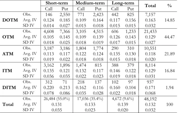
Table 1 reports summary statistics for implied volatilities computed by BS formula adjusted for dividend payments. We divide the data into several categories according to moneyness and time-to-maturity. A put contract is said to be deep-in-the-money (DITM) if m > 0.06; in-the-money (ITM) if 0.06 ≥ m > 0.01; at-the-money (ATM) if 0.01 ≥m ≥ −0.01; out-of-the-money (OTM) if −0.01 > m ≥ −0.06; and deep-out-of-the-money (DOTM) if −0.06 > m. Equivalent deÞnitions apply to calls, with identical bounds but with m replaced with −m in the inequalities. The classiÞcation based on time-to-expiration follows Bakshi et al. (1997): an option contract is short-term if DT E < 60 days; medium-term if 60 ≤ DT E ≤ 180; long-term if DT E > 180 days. Roughly 61% of the data is represented by short- and medium-term OTM and ATM contracts. DITM and long-term contracts are grossly underrepresented.
Table 1 provides evidence on the heterogeneity characterizing S&P 500 implied volatilities as a function of moneyness and time to expiration. For call options, implied volatilities describe an asym-metric smile for short-term contracts, and perfect skews (i.e. volatilities increase moving from DOTM to DITM) for medium- and long-term contracts. Similar patterns are observed for puts, with the dif-ference that volatilities decrease when moving from DOTM to DITM: protective (DOTM) puts yield higher prices and thus higher volatilities. Table 1 also shows that the smile is inßuenced by time to maturity: implicit volatilities are increasing in DT E for ATM contracts (calls and puts), while they are decreasing inDT E for DOTM puts and DITM calls.
2
See Section 6 and Hentschel (2003) for measurement error related issues related to the calculation (estimation) of implied volatilities.
3
2.2. Fitting the Implied Volatility Surface
In this section, weÞt an implied volatility model to each cross section of options available each day in our sample. Given the evidence presented above, two factors seem determinant in modeling the implied volatilities for each daily cross section of option contracts: moneyness and time to expiration. In a second stage, we will model and forecast the estimated volatility function coefficients.
Let σi denote the BS implied volatility for contract i, with time to maturity τi (measured as a fraction of the year, i.e. τi ≡DT Ei/252) and strike price Ki. We consider the following time-adjusted measure of moneyness:4 Mi ≡ ln³ Ki exp(rτi)S ´ √τ i .
Mi is positive for out-of-the-money calls (in-the-money puts) and negative for in-the-money calls (out-of-the-money puts).
Each day we estimate the following cross-sectional model for the IVS by ordinary least squares (OLS):
lnσi=β0+β1Mi+β2Mi2+β3τi+β4(Mi×τi) +εi, (1) where εi is the random error term, i = 1, . . . , N, and N is the number of options available in each daily cross section. We use log implied volatility as the dependent variable. This has the advantage of always producing non-negative implied volatilities. We estimated a variety of other speciÞcations (see Pe˜na et. al. 1999). These included models in which the IVS was only a function of moneyness (either a linear or a quadratic function, or a stepwise linear function of moneyness), and models using both the moneyness and time-to-expiration variables, included in the regression in the logarithmic or quadratic form, without any interaction term. We omit the estimation outputs to save space and because these alternative models showed a worseÞt (as measured by their adjustedR2s) than (1).
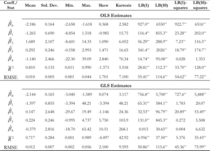
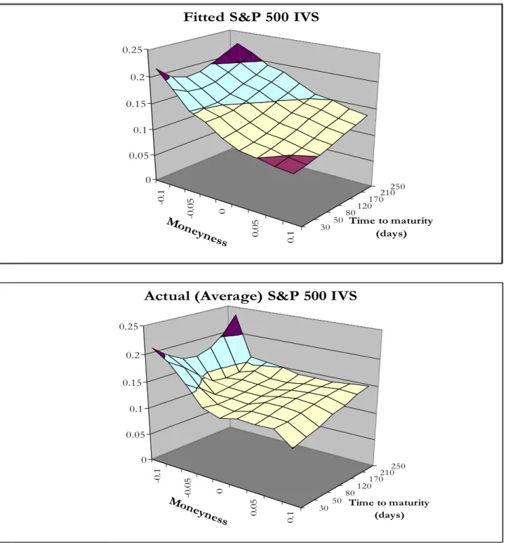
For each day in our sample, we estimate β = (β0,β1,β2,β3,β4)0 by OLS and obtain a vector βˆ of daily estimates.5 To assess the in-sample Þt of our cross-sectional model, we present in Table 2 summary statistics for the adjusted R2 as well as for the RMSE of implied volatilities. On average, the value of ¯R2 is equal to 81%, with a minimum value of 1.1% and a maximum value of 99%. The time series of the daily values of the adjustedR2 and RMSE of implied volatilities (not reported) shows that there is considerable time variation in the explanatory power of equation (1). The functional form implied by this model is nevertheless capable of replicating various IVS shapes, including skews and smiles as well as non-monotone shapes with respect to time to expiration. In the upper panel of Figure 1 we plot the implied “average” Þtted IVS model (i.e. theÞtted model evaluated at the mean values
4Gross and Waltner (1995) and Tompkins (2001) also use a similar measure of moneyness. According to this measure,
the longer the time-to-maturity of an option, the larger the difference should be between the strike price and the forward stock price in order for it to achieve the same normalized moneyness as a short-term option.
5As recently remarked by Hentschel (2003), measurement errors may introduce heteroskedastiticy and autocorrelation
inεi, making the OLS estimator inefficient. In Section 6 we apply the feasible GLS estimator of Hentschel (2003) as a
of the estimated coefficients obtained from Table 2) as a function of moneyness and time-to-maturity. For comparison, in the lower panel of the sameÞgure we present the average actual implied volatilities for each of theÞfteen categories in Table 1, i.e. we plot the average volatility in correspondence to the mid-point moneyness and time-to-maturity characterizing each of the table’s cells. The two plots show close agreement between raw andÞtted implied volatilities.
Figure 2 plots the time series of the daily estimatesβˆ. Figure 2 shows that the shape of the S&P 500 IVS is highly unstable over time, both in the moneyness and in the time to maturity dimensions. Table 2 and Figure 3 contain some descriptive statistics for the estimated coefficients. In particular, the Ljung-Box (LB) statistics at lags 1 and 10 indicate that there is signiÞcant autocorrelation for all coefficients (one exception is ˆβ4), both in levels and squares, suggesting that some structure exists in the dynamics of the estimated coefficients. Figure 3 plots the auto- and cross-correlations for the time series of OLS estimates. The cross-correlograms between pairs of estimated coefficients show strong association between them, at both leads and lags as well as contemporaneously. This suggests the appropriateness of multivariate models for the set of estimated cross-sectional coefficients, whose speciÞcation and estimation we will consider next.6
3. Modeling the Dynamics of the Implied Volatility Surface 3.1. The Model
In this section we model the time variation of the IVS as captured by the dynamics of the OLS coefficients entering the cross-sectional model analysed previously. More speciÞcally, weÞt VAR models to the time series of OLS estimatesnβˆtoimplied by equation (1), where βˆt denotes dayt’s coefficient estimates. Our approach is a reduced form approach to modeling the time variation in the implied volatility surface that results from more structural models such as the investors’ learning models of option prices. In particular, if the state variables that control the dynamics underlying the fundamentals in these models are persistent and follow a regime switching model (such as in David and Veronesi (2002) or Garcia, Luger and Renault (2003)), a VAR model appears to be a reasonable reduced form approach to model the predictability in the implied volatility surface.
We consider the following multivariate model for the vector of estimated coefficientsβˆt: ˆ βt=µ+ p X j=1 Φjβˆt−j+ut, (2) whereut∼i.i.d. N(0,Ω).
For later reference, letπ denote the vector containing all parameters (including the elements of Ω) entering (2). Equations (1) and (2) describe our two-stage, dynamic IVS model. We selectp using the
6Although the mapping between the persistence of the cross-sectional coefficients and the persistence of (log-) implied
volatilities is a complicated one, for ATM contracts the mean-reversion speed is well-approximated by the autocorrelation function ofβ0 and appears to be consistent with an AR(1) model with autoregressive coefficient of 0.9. This estimate is
lower than the volatility mean reversion parameter reported for instance by Heston and Nandi (2000). However, we note that Heston and Nandi (2000) study the volatility of the underlying (in levels), not implied volatilities. Christensen and Prabhala (1998) study log-implied volatilities andÞnd an autoregressive coefficient of 0.7.
BIC criterion, starting with a maximum value ofpequal to 12. This is our main model (which we label Model 1).7 For comparison purposes, we consider DFW’s (1998) ad-hoc strawman, which has proven to
be hard-to-beat in out-of-sample horse races. Christoffersen and Jacobs (2004) have recently employed this benchmark to show that once the in-sample and out-of-sample loss functions used in estimation and prediction are correctly ‘aligned’, this practitioners’ Black-Scholes model is hard to outperform even using state-of-the-art structural models. This model (henceforth Model 2) is a special case of equation (2) when µ = 0, p = 1, Φ1 = I5, a 5×5 identity matrix, Φj = 0 for j = 2, ..., p, and Ω a diagonal matrix. It is a random walk model in whichβˆt=βˆt−1 plus an i.i.d. random noise vector, i.e. the best forecast of tomorrow’s IVS parameters is today’s set of (estimated) coefficients.
We estimate Model 1 by applying OLS equation-by-equation. For comparison purposes, we also estimate on our options data a third structural model, Heston and Nandi’s (2000) NGARCH(1,1). Heston and Nandi (2000) report the superior performance (in- and out-of-sample) of this model over DFW’s ad-hoc strawman when estimated on weekly S&P 500 options data for the period 1992-1994. In contrast to the dynamic IVS models considered here, the NGARCH(1,1) model does not allow for time varying coefficients (although it implies time-varying risk neutral densities). Thus, it seems sensible to require that Model 1 be able to perform at least as well as Heston and Nandi’s NGARCH. We estimate Heston and Nandi’s (2000) model by minimizing the sum of the squared deviations of the BS implied volatilities from the BS implied volatilities derived by “inverting” the NGARCH(1,1) option prices.8 This is in contrast to Heston and Nandi (2000), who apply a nonlinear least squares (NLS) method to option prices directly. By estimating Heston and Nandi’s (2000) model in the implied volatility space, we preserve the consistency with the dynamic IVS models.9
3.2. Estimation Results
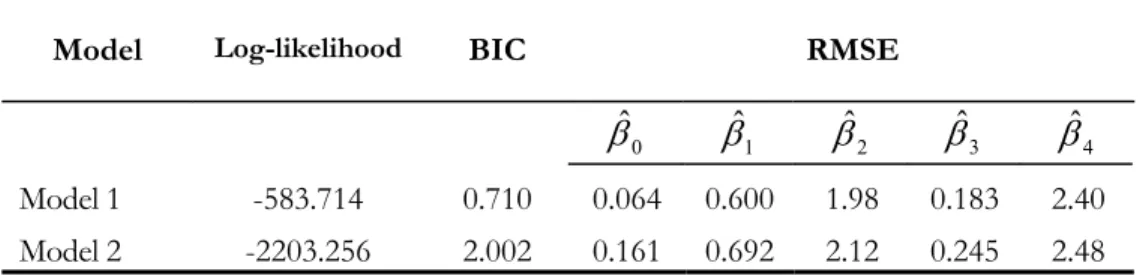
Table 3 reports estimation results for Models 1 and 2, Þtted to the parameter estimates from the cross-sectional model described by equation (1). Model 1 outperforms the more parsimonious Model 2 in-sample, as signalled by its high value for the log-likelihood function and the smallest RMSE values for theÞrst-step parameter estimatesβˆt.We will evaluate the two models out-of-sample to account for the possibility that the superior performance of Model 1 is due to overÞtting the data.
7
(2) allows for a variety of dynamic speciÞcations of the implied volatility surface (as described by the cross-sectional coefficient estimatesβˆt), depending on the choice of pand on the restrictions imposed on its coefficients. In an earlier version of this paper, we considered two further model speciÞcations: one in which the lag order was selected by a sequential likelihood ratio testing algorithm, and one in which exogenous information in the form of lagged returns on the S&P 500 index entered the VAR model. Since the out-of-sample performance of these models turned out to be inferior to Model 1, we omit related results (see Gon¸calves and Guidolin (2003) for details).
8
We obtained the following estimates: rt = rf − 12 √ ht + √ htz∗t, with ht = (0.83 × 10⁻⁶) + (0.67 × 10⁻⁶)£zt∗−1+ ¡1 2 + 316.5 + 2.45 ¢√ ht−1¤ 2
+ 0.91ht−1, where we use notation similar to Heston and Nandi (2000). The
implied nonlinear GARCH process has high persistence (β+αξ2 = 0.98), as typically found in the literature (Heston
and Nandi (2000) found persistence levels of roughly 0.9-0.95 on their S&P 500 index options weekly data). Also the estimate of the risk premium is standard (Heston and Nandi’s estimates are between 0.5 and 2). The NGARCH(1,1) models reaches an average root-mean squared implied volatility error of 2.01%, which is quite impressive considering that the model speciÞesÞve parameters only.
9
In order to obtain an idea of the predictions implied by our two-stage IVS model, Figure 4 plots the sequence of IVS snapshots over the period January 3, 1992 through June 28, 1996 implied by Model 1’s estimates. In particular, in the Þrst row we plot Þtted implied volatilities against time and moneyness, given two distinct maturities (DT E= 30 andDT E = 120), whereas in the second row we plot Þtted implied volatilities against time and maturity, given two distinct moneyness levels (m = 0 and m = 0.05, i.e. ATM and ITM puts (and ATM and OTM calls)). Figure 4 shows that Model 1 is capable of generating considerable heterogeneity in the implied volatility surface, consistent with well-known stylized facts: skews for short-term contracts; relatively higher implied volatilities in 1992, early 1994 and at the Spring of 1996; less accentuated skews, which become asymmetric smiles when higher implied volatilities are observed, etc. For medium-term contracts, Model 1 implies instead a
ßatter and practically linear IVS; skews dominate.
The bottom row of plots in Figure 4 shows that some heterogeneity affects also the Þtted IVS in the term structure dimension. Although positively sloping shapes dominate, ßat and even downward sloping schedules occasionally appear. For instance, between the end of 1992 and early 1993, theÞtted term structure is steeply upward sloping, implying volatilities in the order of almost 30% for ATM, long-term contracts (vs. 10% for short-term ones); on the opposite, early 1995 is characterized byßat term structures. For ITM puts (OTM calls), weÞndßatter schedules on average, although substantial heterogeneity remains. Interestingly, in this case many schedules are actually non-monotone, i.e. they are at Þrst decreasing (for very short maturities, less than one month) and then slowly increasing in time to expiration. We interpret Figure 4 as evidence of the possibility to accurately model not only the cross-sectional structure of the S&P 500 IVS but also its dynamics. The conceptually simple vector autoregressive Model 1 provides a very goodÞt and produces implied volatility surfaces that are plausible both in their static structure and in their evolution.
4. Statistical Measures of Predictability
Our approach to modeling the IVS dynamics proves successful in-sample, as previous results show. Nevertheless, a good model of the IVS should not only Þt well in-sample, but also provide good out-of-sample predictions. The main goal of this section is thus to analyze the out-out-of-sample forecasting performance of Models 1 and 2 at forecasting one-step ahead, daily implied volatilities (and option prices). For comparison purposes, we include Heston and Nandi’s (2000) NGARCH(1,1) model, as well as a random walk model for daily implied volatilities (henceforth called the ‘random walk model’). According to this random walk model, today’s implied volatility for a given option contract is the best forecast of tomorrow’s implied volatility for that same contract. Harvey and Whaley (1992, p. 53) comment that “(...) while the random walk model might appear naive, discussions with pratictioners reveal that this model is widely used in trading index options.”
We estimate each of the models using data for the periods January 1, 1992 through December 31, 1992; January 1, 1992 - December 31, 1993; and so on, up to January 1, 1992 - December 31, 1995. This yields four distinct (and expanding) estimation windows. For each day in a given estimation window, we estimate the cross-sectional IVS parameters βt by OLS. We obtain a time series nˆβto, which we then use as raw data to obtain estimates ofπ, the parameters of the multivariate models described by (2). We
allow the model’s speciÞcation (e.g. the number of lagsp) to change in each estimation window. For the NGARCH(1,1) benchmark, we follow Heston and Nandi’s (2000) approach and estimate its parameters (which we also denote byπ to simplify notation) by NLS, except that our objective function is deÞned in the implied volatility space. Letπˆ denote the parameter estimates for each of these models and for a given estimation window. We then holdπˆ constant for the following six months – i.e. January 1, 1993 through June 30, 1993; January 1, 1994 - June 30, 1994, etc. up to January 1, 1996 - June 28, 1996 – and produce daily one-step ahead forecasts of the estimated coefficientsβˆ. Because the IVS on dayt+ 1 depends onβˆt+1, forecasting βˆt+1allows us to forecast implied volatilities (and option prices) for each of these four six-month prediction windows, given moneyness levels and time-to-maturity. Importantly, non-overlapping estimation and prediction windows guarantee that only past information on the dynamic properties of the S&P 500 IVS are used for prediction purposes.
To assess the out-of-sample performance of the Þtted models for the second half of each of the four years under consideration, each day in a given prediction window we compute the following six measures for each model:
(i) The root mean squared prediction error in implied volatilities (RMSE-V) is the square root of the average squared deviations of BS implied volatilities (obtained using actual option prices) from the model’s forecast implied volatilities, averaged over the number of options traded.
(ii) The mean absolute prediction error in implied volatilities (MAE-V) is the average of the absolute differences between the BS implied volatility and the model’s forecast implied volatility across traded options.
(iii) The mean correct prediction of the direction of change in implied volatility (MCP-V) is the average frequency (percentage of observations) for which the change in implied volatility predicted by the model is of the same sign as the realized change in implied volatility.10
(iv) The root mean squared prediction error in option prices (RMSE-P) is computed as in (i) but with reference to option prices.
(v) The mean absolute prediction error in option prices (MAE-P) is computed as in (ii) but with reference to option prices.
(vi) The mean correct prediction of the direction of change of option prices (MCP-P) is computed as in (iii) but with reference to option prices.
In computing (iv) - (vi) above, we compare actual option prices with the model’s forecast of option prices. We use the BS formula to compute the model’s forecast of option price, using the corresponding implied volatility forecast as an input (conditional on the current values of the remaining inputs such as index value, interest rate and the contract’s features). Our use of the BS model is obviously inconsistent with the volatility being a function of moneyness and/or time to maturity. Nevertheless, such a pricing scheme is often used by market makers (cf. Heston and Nandi (2000)). It is our goal here to see whether
a theoretically inconsistent but otherwise ßexible approach can deliver statistically and economically signiÞcant forecasts. We follow Harvey and Whaley (1992) and view our IVS models as a “black box”, which is Þrst used to obtain implied volatilities from option prices for forecasting purposes, and then transforms implied volatilities back into prices.11
Table 4 (panel A) contains the average values of the out-of-sample daily performance measures (i) - (vi) aggregated across all four out-of-sample periods.12 The aggregated out-of-sample root mean squared error in annualized implied volatilities is 1.43%, 2.30%, 2.07% and 1.49% for Models 1 and 2, the NGARCH(1,1) model and the random walk model, respectively. The values for the out-of-sample measures related to forecasting option prices are $1.00, $1.75, $1.71, and $1.64, respectively. The best performing model according to these measures is Model 1, the VAR model forβˆt. Similar results are obtained in terms of average percentage of correct predictions for the sign of the change of volatilities between two consecutive trading days: the best performance is provided by Model 1 (62.2%), followed by Model 2 (55.8%). Modeling the dynamics of the IVS offers real advantages over a simpler, static DFW-type speciÞcation (Model 2) in which the structure of the IVS is predicted not to change from one day to the next. Model 1 also compares favorably with the two benchmarks considered, outperforming both the NGARCH(1,1) model and the practitioners’ random walk model for implied volatilities. Similarly to Heston and Nandi (2000), weÞnd that the NGARCH(1,1) model outperforms Model 2.13
To formally assess the statistical signiÞcance of the difference in out-of-sample performance of Model 1 compared to each of the remaining models, we employ the equal predictive ability test proposed by Diebold and Mariano (1995). We consider three types of performance indicators: the difference in squared forecast errors (corresponding to measures (i) and (iv)); the difference in absolute forecast errors (corresponding to measures (ii) and (v)); and the difference between two indicator functions, where each indicator function takes the value one if the realized change in the variable being predicted (e.g. the implied volatility) has the same sign as the predicted change (i.e. the forecast error), and zero otherwise. This last performance indicator is consistent with the out-of-sample measures given in cases (iii) and (vi). To compute the Diebold and Mariano (1995) test, we use the Newey-West (1987) HAC (heteroskedasticity and autocorrelation consistent) variance estimator. Table 4 (panel B) reports the values of the statistic and associated signiÞcance levels. With very few exceptions, we reject the null hypothesis of equal forecast accuracy of Model 1 compared to the benchmark models. We conclude that the out-of-sample superior performance of Model 1 is statistically signiÞcant. Moreover, in the
11The forecasting exercises underlying our computation of the performance measures (iv) through (vi) are subject to
Christoffersen and Jacobs’ (2003) critique that the loss function used in estimation (based on implied volatility matching) differs from the out-of-sample loss function (based on BS option prices). Since BS is non-linear in implied volatility, severe biases may be introduced. Based on the results of Christoffersen and Jacobs’ (2003), we expect that the use of the “correct loss” function in estimation will reduce the values of the out-of-sample statistics in Table 4 for our approach.
12Note that it is not possible to calculate the mean percentage of correct prediction of the direction of change of implied
volatility for the random walk model since this model implies zero predicted changes in implied volatility by construction.
13
In unreported results, we also studied out-of-sample performance for each of the four prediction windows. The overall picture remains favorable to our approach, although years of higher volatility and turbulent markets (like 1994) deteriorate the performance of our approach. We also investigated the forecasting accuracy in multi-step ahead forecasting. We considered horizons of 2, 3 and 5 trading days. The ranking across models remains identical to the one from Table 4: Model 1 outperforms Model 2 and the NGARCH(1,1) benchmarks at all horizons. However, although superior, the accuracy of Model 1 declines faster than Model 2 and the NGARCH as the prediction horizon is increased.
rare occasions in which Model 1 underperforms the benchmarks, the difference is not only rather small in absolute terms, but we cannot reject the hypothesis of equal predictive accuracy.
The superior out-of-sample performance of Model 1 relative to Model 2, the static ad hoc model heavily used by practitioners, conÞrms that time variation in the implied volatility surface is statis-tically important. Importantly, economic models of the IVS such as those that allow for investors’ learning to affect equilibrium option prices can explain these Þndings. If on a learning path beliefs are persistent because the updating occurs in a gradual fashion, the stochastic discount factor should inherit these properties and imply predictability of the IVS. This implies that Model 2 which ignores such predictability − i.e. a random walk for the Þrst-stage coefficients − has a hard time capturing the dynamics of the IVS. Instead, Model 1 represents a reduced form framework able to capture the dynamic properties of the IVS. As often documented in forecasting applications, such a reduced form approach works very well, outperforming the more complex structural model of Heston and Nandi (2000).
In order to further analyze the nature of the forecasting ability of Model 1, Table 5 reports out-of-sample average prediction errors by different option moneyness and maturity categories. SpeciÞcally, for each category we report the average out-of-sample root mean squared error for implied volatilities (and option prices), expressed as a percentage of the mean implied volatility (and mean option price) in that category. Scaling by mean volatility and price is important to gain comparative insight on the sources of Model 1’s out-performance. For comparison purposes, we also include Model 2, the restricted (static) version of the moreßexible dynamic Model 1. In addition, we consider a simple AR(1) model for (log-) implied volatilities, as in Christensen and Prabhala (1998). Contrary to Model 1, this model does not exploit the panel structure of options data as it applies to a single time series of (log-) implied volatilities. In particular, for a given options class, we create a time series of (log-) implied volatilities by selecting each day the contract that is closest to the mid-point in this category.14 Since this simple AR(1) model does not utilize any cross-sectional restrictions on implied volatilities, we expect it to perform worse than Model 1.
Our Þndings are as follows. We start with Model 1. For any given moneyness level, medium-term contracts are associated with the smallest prediction errors, both in implied volatilities and in option prices. The ranking between short-term and long-term contracts depends on moneyness. For in-the-money and ATM options, long term contracts have smaller prediction errors than short-term contracts (in both the volatility and price metrics). For out-the-money options the opposite is true. For a given maturity level, RMSE’s (in volatilities and option prices) are generally decreasing when moving from DITM to DOTM, i.e. it is easier to predict out-the-money than in-the-money implied volatilities and option prices. The only exception to this pattern is when forecasting implied volatilities for long term
14
For a given options class, on each day for which there are options available in that class we select the contract that solves the following problem:
min mi,τi · (mi−mc)2 σ2 m +(τi−τc) 2 σ2 τ ¸ ,
wheremc andτcare the mid-points of the moneyness and maturity intervals deÞning the class, andσ2m andσ2τ are the variances of moneyness and time to expiration for all contracts in the class traded that day.
contracts, for which a U-shaped pattern of RMSE-V emerges.
In sum, the forecasting strength of Model 1 seems to originate mainly from the short- and medium-term, out- and at-the-money segments of the market.
For the AR(1) model, RMSE’s tend to decrease with maturity, given moneyness. One exception is the DOTM class, for which short-term options have the lowest RMSE-P. For any maturity level, the AR(1) model achieves in general lower RMSE-V for ATM implied volatilities than in-the-money or out-of-the-money contracts. For short-term and medium term options, the RMSE-P decreases mono-tonically when moving from DITM to DOTM.
Table 5 shows that Model 1 generally beats the AR(1) model across all moneyness and time to expiration classes.15 Thus, the gain in forecasting from our two-stage approach seems to come from the cross-sectional restrictions. The greatest improvements in RMSE-V occur for out-the-money, short-and medium-term contracts; instead, the greatest gains in RMSE-P occur for in-the-money, short- short-and medium-term contracts. The smallest gains are obtained for ATM contracts. This conÞrms that the additional information contained in the segments of the IVS far from at-the-money may be crucial in improving the forecasting performance of IVS models.
Model 1 also outperforms Model 2 for all categories. The largest reductions in average prediction errors are obtained for ATM and out-the-money, short- and medium-term options, when forecasting implied volatilities, whereas ATM and in-the-money, short- and medium-term options show the largest reductions in RMSE-P. DITM options are in general associated with smaller reductions in implied volatilities prediction errors, suggesting that for this class of options the dynamics in the coefficients capturing the IVS shape is stable enough to allow accurate forecasting from Model 2.
For out-the-money, short- and medium-term options, Model 2 yields lower average prediction errors than the AR(1) model, which suggests that for these classes it is more important to model the cross-section dimension of the options data than the time series dimension. Instead, for ATM options, the simple AR(1) model outperforms Model 2, suggesting that it is important to model the dynamics of implied volatilities for this class of options.
5. Economic Analysis
The results of Section 4 suggest that implied volatilities (and corresponding option prices) are highly predictable in a statistical sense. The good out-of-sample statistical performance of our model, and the fact that our approach can be viewed as a reduced-form approach that captures the dynamics in the IVS that could be generated by equilibrium-based economic models suggest some robustness of our results to data mining. However, we cannot exclude entirely the possibility that our results are subject to mining biases. Therefore, as an additional test, we now examine the economic consequences and signiÞcance of this predictability. In particular, we ask: Would a hypothetical market trader be able to devise any proÞtable trading strategies based on the implied volatility forecasts produced by our two-stage dynamic IVS models? We follow Day and Lewis (1992), Harvey and Whaley (1992), and Noh, Engle and Kane (1994) and evaluate the out-of-sample forecasting performance of a number of
15The AR(1) model outperforms Model 1 only in two cases: for ITM, long-term options (when it achieves a smaller
competing models by testing whether certain trading rules may generate abnormal proÞts, i.e. proÞts that are not accounted for by the risk of the positions required by the strategies.16
5.1. Trading Strategies and Rate of Return Calculations
The trading strategies we consider are based on out-of-sample forecasts of volatility. More speciÞcally, if on a given day implied volatility is predicted to increase (decrease) the following day, the option is purchased (sold). Each day we invest $1,000 net in a delta-hedged portfolio of S&P 500 index options, which is held for one trading day.17 The trading exercise is repeated every day in the out-of-sample period and a rate of return is calculated.
Implied volatility forecasts are obtained as in Section 4: on daytwe use the time series of estimated coefficients βˆ describing the IVS, up to and including day t, to predict day’s t+ 1 coefficients βˆt+1
by means of the VAR-type models estimated from the appropriate estimation window. The forecast of ˆβt+1 is then used to predict day’s t+ 1 implied volatility associated with a given option. Since the index price and interest rate att+ 1 are not known as of timet, we assume that today’s prices of the primitive assets are tomorrow’s best forecasts. To delta hedge our options position, per each unit of call (put) options bought, we sell (buy) an amount of the underlying index equal to the Black-Scholes delta ratio (∆), calculated using the implied volatility forecast. Similarly, if we sell one call (put) option, we buy (sell) an amount of the underlying index equal to the corresponding Black-Scholes hedge ratio.18
To compute the rate of return, we assume funds may be freely invested at the riskless interest rate. Suppose that one particular trading rule has indicated that a certain subset of contractsQ should be traded at time t. Let Cit denote the price of a call contract i at time t and Pit the price of a put contracti at time t. The delta ratios corresponding to call and put options are denoted ∆C
it and ∆Pit, respectively. If no options are traded (i.e. Q is empty), we force the trader to invest her $1,000 in the riskless asset for one trading period. We distinguish between two cases: aÞrst case in which the overall timetnet cost of the delta-hedged portfolio is positive, and a second case in which the cost is negative. ConsiderÞrst the case in which the portfolio requires an injection of funds. LetVtdenote the price of a unit portfolio in which all contracts are sold or purchased in one unit:
Vt= X i∈Qcall + ¡ Cit−St∆Cit ¢ + X i∈Qput+ ¡ Pit+St∆Pit ¢ − X i∈Qcall ¡ Cit−St∆Cit ¢ − X i∈Qput ¡ Pit+St∆Pit ¢ , (3)
whereQcall+ (Qcall− ) is the subset ofQ for which a buying (selling) signal on calls was obtained; similar deÞnitions apply to puts. Then $1,000 are invested in a portfolio in which all options in Q (and their
16These experiments might be also constructed as tests of the informational efficiency of the S&P 500 index options
market. An efficient market ought to be able to produce option prices consistent with the implied volatility forecasts from our two-step estimation procedure. If abnormal proÞts can be made, the efficient market hypothesis is rejected. Alternatively, the most likely explanation is to be found in microstructural features that make the underlying index and option prices adjust to theßow of news at different speeds.
17
Delta hedging is intended to render the portfolio’s value insensitive to market movements so that our computed proÞts truly reßect proÞts in ‘trading in volatility’.
18
In practice hedging is accomplished by trading in S&P 500 futures with appropriate maturities. The resulting hedging is imperfect as the underlying consists of the spot index, and index and futures fail to be perfectly correlated (basis risk). For the sake of simplicity we ignore the complications arising from hedging with futures.
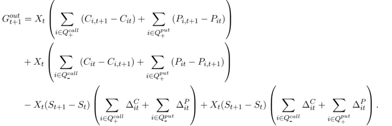
associated delta hedging positions in the S&P 500 index) are traded in the quantityXt= 1,V000t , with a total cost of $1,000. Hence the resulting portfolio is value-weighted. The net gain betweentand t+ 1 can be determined as:
Goutt+1=Xt X i∈Qcall + (Ci,t+1−Cit) + X i∈Qput+ (Pi,t+1−Pit) +Xt X i∈Qcall (Cit−Ci,t+1) + X i∈Qput+ (Pit−Pi,t+1) −Xt(St+1−St) X i∈Qcall + ∆Cit + X i∈Qput ∆Pit +Xt(St+1−St) X i∈Qcall ∆Cit + X i∈Qput+ ∆Pit . (4) Next, consider the case in which the portfolio generates cash inßows, e.g. most or all of the trading signals are selling signals. DeÞne Vt as in (3), except for the fact that now Vt < 0. In this case a portfolio worth $1,000 is created by trading each contract for which there exists an active signal in the quantityXt= 1|,V000
t| .We assume that the $1,000 option portfolio generated inßows plus the additional
$1,000 originally available are invested at the riskless interest ratert. The resulting net gain between tand t+ 1 can be calculated in a manner similar to (4):
Gint+1 =Goutt+1+ 2,000 exp(rt/252).
We consider several trading rules. In order to avoid noisy signals, all our trading strategies use a price deviation Þlter of 5 cents.19 This implies that trading occurs only when the price difference between the predicted option price (i.e. the BS predicted price based on our volatility forecast) and today’s observed price is larger than theÞlter.20 First, following Harvey and Whaley (1992), we consider a trading rule (henceforthTrading Rule A) in which trades only occur on closest-at-the-money, shortest-term contracts (thusQ≤1). Second, we consider a strategy (Trading Rule B) for which trading occurs only in two contracts, those for which the expected selling and the expected buying proÞts, respectively, are maximum. In this caseQ≤2 obtains at all times. In a third set of simulations (Trading Rule C), we consider trading only in one contract, the one giving the highest expected trading proÞt, so that Q≤1 again.
5.2. Trading ProÞts Before Transaction Costs
Table 6 presents summary statistics for proÞts deriving from Trading Rules A-C. We consider two mea-sures of abnormal returns (proÞtability): the Sharpe ratio and a risk measure due to Leland (1999). The Sharpe ratio is an appropriate measure of proÞtability when investors have mean-variance preferences.
19
Later we will increase the value of thisÞlter.
20
Since the theta of a European option (the rate of change of its value as time to maturity decreases) is normally negative, comparing predicted and current implied volatilities contains a small bias, in the sense thatceteris paribus the option price implied by predicted volatility will be normally slightly smaller than the current price because of the mere passage of time. By applying some minimalÞlter to the differences in implied prices adjusts for this bias.
This is hard to rationalize under non-normal returns. Instead, Leland’s (1999) risk measure allows for deviations from normality by taking into account skewness, kurtosis and other higher-order moments of the returns distribution. It derives from a marginal utility-based version of the single-period CAPM, as follows: A=E · Gt+1 1,000 ¸ −rt−B(E[rmkt]−rt),
where rmkt denotes the return on the market portfolio and B is conceptually similar to a preference-based CAPM beta (under power utility). Crucially, a positiveAindicates performance which is abnor-mal even when the features of higher-order moments (like negative skewness or excess kurtosis) of the empirical distribution of trading proÞts are taken into account. Appendix 1 provides further details on the calculations underlyingA and its inputs.
Three benchmarks are considered. One is the random walk model for implied volatilities. Since this model predicts tomorrow’s implied volatility to be equal to today’s value, it does not provide buy or sell signals, and therefore the resulting strategies trivially correspond to buying and holding T-bills every day in the prediction window. In this case, mean proÞts are negligible and the Sharpe ratio is zero by construction. One might wonder whether it is simply possible to make abnormal proÞts by randomly trading option contracts. We therefore include a random (delta-hedged) buy & sell option strategy as a benchmark: according to this rule, each option has a 0.5 probability of being traded; if selected, the option is sold with probability 0.5, otherwise it is purchased. The third benchmark we consider is the “S&P 500 Buy & Hold” rule, by which each day the $1,000 are simply invested in the underlying S&P 500 index, thus obtaining Sharpe ratios andA coefficients which are typical of the CAPM.
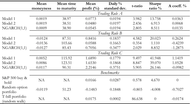
Table 6 shows that our two-step approach to modeling and forecasting the S&P 500 IVS is successful at generating proÞtable strategies. Indeed, Model 1 yields statistically signiÞcant positive mean proÞts under all three trading rules. Trading Rule A, based on trading the closest ATM, shortest maturity contract, implies a daily mean proÞt of 0.083%, with at-ratio of 4.2, followed by Trading Rule C (mean proÞt equal to 1.322% and t-ratio equal to 11.03) and by Trading Rule B (mean proÞt of 2.18%, with at-ratio equal to 3.9). As expected, Trading Rule A is less successful than the remaining trading rules as it is constrained in terms of moneyness. All trading rules yield Sharpe ratios that easily outperform the 4.7 ensured by the S&P 500 buy-and-hold strategies, i.e. they do reward risk in excess of the market portfolio. This conclusion is robust to the CAPM-based performance evaluation delivered by the coefficient A for Trading Rules A and C, for which A is positive. For Trading Rule B, a negative value ofA is obtained, despite the large value of the Sharpe ratio (17.4). The empirical distribution of trading proÞts for this trading rule reveals that it is associated with very high values of excess kurtosis, which is negatively weighted under theAcoefficient. Since the Sharpe ratio only takes into account the mean and variance of proÞts, it fails to include this feature, explaining the large value obtained. The negative value ofA suggests that daily rewards in excess of 2% per day are insufficient to compensate for the risk absorbed under Trading Rule B.
A comparison between Model 1 and the remaining models reveals that Model 1 yields in general higher mean daily proÞts than Model 2 and NGARCH(1,1). One exception is Trading Rule C, for which the NGARCH(1,1) model performs best, yielding a mean proÞt of 2.21% per day, against mean
proÞts of 1.35% for Model 2 and 1.32% for Model 1. Nevertheless, the high proÞts obtained by the NGARCH(1,1) under Trading Rule C are abnormally low as signalled by a negative value ofA. Instead, Models 1 and 4 are associated with large values of Sharpe ratios and positive values ofA, suggesting that their performance is truly abnormal.
5.3. Trading Results After Transaction Costs
The results from Section 5.2 suffer of two limitations. First, they ignore the effect of transaction costs. Second, Trading Rules A-C may be so narrowly deÞned as to imply that a very limited (typically, Q = 1) number of contracts are traded. Therefore, it is possible that a model that poorly predicts volatilities and prices out-of-sample, does manage to provide correct buy and sell signals, either for ATM short-term contracts or for the most aberrant misspricings (maximizing expected proÞts).
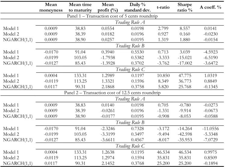
Table 7 presents results that take transaction costs into account. We re-compute rate of returns for Trading Rules A-C when the payment of aÞxed transaction cost per contract traded (both options and the S&P 500 index) is imposed. We apply two different levels of unit cost, $0.05 (Panel 1) and $0.125 (Panel 2). Panel 1 shows that low transaction costs barely change the conclusions reached in Table 6. As expected, after-transaction costs proÞts are lower on average, but the ranking of models is the same as in Table 6. Model 1 outperforms Model 2 and the NGARCH(1,1) for Trading Rules A and B, achieving the highest daily mean percentage proÞts and Sharpe ratios. For Trading Rule C, Model 1’s performance is similar to that of Model 2. Although both models yield lower daily mean proÞts than the NGARCH(1,1) model, they both guarantee positive A coefficients, with Model 1 achieving the largest percentage abnormal return. In contrast, the NGARCH(1,1) implies a negative value ofA. To test the robustness of our results, Panel 2 increases transaction costs to $0.125 per traded contract (round-trip). In this case, positive and signiÞcant mean daily proÞts result for all models under Trading Rule C, with the best performing model being the NGARCH(1,1) model, followed by Model 2 and Model 1. As before, the performance of the NGARCH(1,1) model cannot be considered abnormal as signalled by the (negative) value of theA coefficient, whereas the performance of Models 1 and 2 can. None of the models is nevertheless able to produce signiÞcantly positive proÞts under the other two trading strategies (Trading Rules A and B).
One of the strengths of our two-step approach is that it allows to model and forecast the entire S&P 500 IVS. The trading rules analyzed thus far are designed to pick a small number of option contracts (typicallyQ= 1 or 2), and therefore do not exploit entirely theßexibility provided by our approach. In order to allow for trade in a larger set of option contracts, we introduce a fourth type of trading strategy (Trading Rule D), which applies Þlter rules to the price deviation for selecting options to be traded. In particular, we considerÞlters equal to $0.125, $0.25, and $0.50, and allow trades in all contracts for which the absolute value of the price deviation exceeds the Þlter. Under these Þlter arrangements, Q can contain a large number of contracts, not being constrained to be at most one or two contracts, as in Trading Rules A-C. In addition to the price Þlters, we apply transaction costs of the same magnitude on each contract traded on a round-trip basis, as in Table 7.21 High transaction costs such as $0.50
21Transaction cost-basedÞlter strategies (i.e. strategies that discount the presence of a cost that is actually to be paid
are designed to represent the situation faced by retail customers, who often pay substantial commission fees in addition to the bid-ask spread.
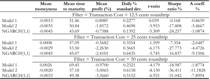
Table 8 reports the results for Trading Rule D. It shows that the proÞtability ofÞltered-based trading rules depends heavily on the magnitude of theÞlter/transaction cost employed. For aÞlter/transaction cost of $0.125, Model 1 is the only model that is able to guarantee signiÞcant (statistically and econom-ically) positive proÞts. This is in contrast with the static IVS model (Model 2) and the NGARCH(1,1) model, which predict negative (statistically signiÞcant) proÞts. Results, not reported here, show that most of Model 1’s proÞts come from trading short-term ATM and OTM contracts. Instead, DITM contracts yield losses on average, with proÞts being statistically signiÞcantly negative for medium-term contracts. This is consistent with our previous Þndings of smaller RMSE-P for out-of-the-money as compared to in-the-money options for Model 1 (cf. Table 5). When we increase theÞlter/transaction cost to $0.25,Model 1 predicts positive proÞts, but these are not statistically signiÞcant, the implied Sharpe ratio is single-digit, below what would be guaranteed by a simple buy & hold daily strategy applied to the S&P 500 index, and the value ofAbecomes negative. All models predict negative proÞts when theÞlter/transaction cost of $0.50 is applied. Therefore, it seems that as the level of transaction costs is progressively raised above $0.25 (on a round-trip basis), mean daily proÞts for all models dis-appear, i.e. for the levels of frictions that are most likely to be faced by small (retail) speculators, the strong statistical evidence of predictability in the IVS dynamics fails to be matched by equally strong evidence of a positive economic value.
To shed further light on the relationship between the proÞtability of trading rules that rely on our predictabilityÞndings and transaction costs, we perform a further experiment: we calculate the exact level/structure of transaction costs such that mean daily proÞts are either zero or stop being statistically signiÞcant at conventional levels. In particular, we apply a Þxed $10 commission to all transactions (i.e. an ex-ante -1% return on a $1,000 investment) and proceed to vary the per-contract (round-trip) cost between $0.02 and $0.75. For comparison purposes with Table 8, we apply this range of friction levels to Trading Rule D. We also apply the same structure of transaction costs to the underlying stock index. Results are reported in Figure 5, where the upper panel reports mean daily percentage returns as a function of the per-contract cost, and the lower panel shows related t-statistics. Clearly, the plots illustrate that both mean proÞts and their statistical signiÞcance disappear (and turn negative) as transaction costs are raised. In particular, it seems that for Model 1 proÞts disappear when the cost per contract is around $0.12-$0.14, consistently with theÞndings in Table 8. In practice trading proÞts stop being signiÞcant already for $0.10, while they eventually become signiÞcantly negative for per contract costs of approximately $0.40. Interestingly, Model 1 systematically outperforms both Model 2 and the NGARCH model. In fact, Model 2 never produces signiÞcantly positive proÞts, once theÞxed commission is deducted.22
contain only signals that, at least in expectation, imply positive after-transaction-cost proÞts. On the other hand, and because we apply transactions costs of the same magnitude as theÞlter, they obviously depress after-transaction costs realized proÞts. Which effect turns out to be stronger is an empirical issue. For instance, Harvey and Whaley (1992, table 5)Þnd thathighenough transaction costs used asÞlters induce positive and signiÞcant proÞts (however, their simulation does not apply transaction costs equal toÞlters).
6. Robustness
In this section, we present some additional results intended to check the robustness of our previous
Þndings to two issues. One is the existence of measurement errors in the inputs entering the BS formula (such as the S&P 500 index level and/or in option prices). The second check we consider refers to the effects of bid-ask spreads on the rate of returns calculations.
6.1. Effects of Measurement Errors
Hentschel (2003) has recently stressed that even small measurement errors in option prices or in the S&P 500 index level can produce large errors in implied volatilities for options away from the money. Thus, it is important to investigate whether the presence of such measurement errors is driving our predictability results. As Hentschel (2003) shows, the existence of measurement errors in the underlying prices induces heteroskedasticity and autocorrelation in the errors of the cross-sectional IVS model (equation (1) above). This implies that OLS estimates of β are inefficient. To obtain more efficient estimates of β, and thus of implied volatilities, we follow Hentschel (2003) and re-estimate equation (1), day by day, using a feasible GLS method. The details of the implementation of this method are in Appendix 2.
Table 2 (bottom panel) presents summary statistics for the feasible GLS estimates as well as for the adjusted R2 and RMSE of implied volatilities. The estimates are on average similar to those obtained by OLS, with the exception of ˆβ2 and ˆβ4. The in-sample goodness of Þt (as measured by
¯
R2 and RM SE) deteriorates only slightly under GLS estimation as compared with OLS. As before, the signiÞcant values of the LB statistics indicate that there is strong serial correlation (in levels and squares) in the estimates, suggesting a second stage multivariate modeling approach.
Table 4 (panel A) presents the out-of-sample forecasting measures (i) through (vi) deÞned in Section 4 when the GLS estimates are used as the raw data in the second-stage. On average, the RMSE and MAE of implied volatilities are slightly higher for all models, although interestingly the pricing RMSE and MAE are often lower than those obtained by OLS. Model 1 remains the best model out-of-sample, yielding a RMSE-V of 1.516 (vs. 1.429 under OLS) and a RMSE-P of 93 cents (vs. $1 under OLS). It still clearly outperforms the benchmarks in terms of BS pricing (MAE-P and RMSE-P) and percentage accuracy at predicting the direction of change.
In Table 9 we present summary statistics for trading proÞts before transaction costs for Trading Rules A-C under GLS estimation. As obtained before under OLS (cf. Table 6), Model 1 performs best for Trading Rules A and B, yielding the highest average proÞt rates, with statistically signiÞcantt-ratios, large Sharpe ratios and positive values of A. However, the use of GLS estimates implies a reduction on the mean proÞts for these trading rules, which is especially large in the case of Trading Rule B (the mean proÞt is now equal to 0.84% per day whereas before it was equal to 2.18%). Interestingly, for Trading Rule C, Models 1 and 2 yield higher mean proÞts under GLS than under OLS.
Table 10 shows that these results are largely robust to the introduction of transaction costs, similarly the impliedÞlters are also increased in a way that makes trading (under rule D) more selective and possibly more proÞtable. This explains theßat (or even upward sloping) segments generally obtained for intermediate costs, $0.30 - $0.40.
to Table 7. Even a commission fee of 12.5 cents per contract fails to completely remove the proÞtability of some of the trading rules, especially the selective rule C. Surprisingly enough, GLS estimation does even increase mean daily returns for Trading Rule C. ThisÞnding suggests that efficient estimation of the IVS may be important to improve the prediction accuracy in the segments of the IVS over which selective trading rules are most likely to produce buy and/or sell signals.
6.2. Effects of Bid-Ask Spreads
Although we have attempted to take into account the effects of transaction costs in computing trading proÞts, we have so far ignored the effects of bid-ask spreads as our simulated trading strategies have used observed closing prices (calculated as mid-points of the spread). Since actual transactions would have to take place inside the bid-ask spread but not necessarily at its midpoint, it is reasonable to assume that on average half of the bid-ask spread must be incurred as an additional transaction cost in the options market when a trade takes place, in addition toÞxed commission costs. In this section, we try to take into account the effects of bid-ask spreads in our rate of return calculations.
Given that our data set does not include bid-ask spreads, we resort to DFW’s (1998) data set, which contains (transaction-based) information on bid-ask spreads at a weekly frequency (every Wednesday).23 In order to complete our data set, we impute to all days within the same week of each Wednesday in DFW’s data set the bid-ask spreads sampled for that Wednesday.24 Daily returns are computed as before, with the difference that we now simulate purchases at the ask (minus one qu