Stock Market Declines and Liquidity
ALLAUDEEN HAMEED, WENJIN KANG, and S. VISWANATHAN*
ABSTRACT
Consistent with recent theoretical models where binding capital constraints lead to sudden liquidity dry-ups, we find that negative market returns decrease stock liquidity, especially during times of tightness in the funding market. The asymmetric effect of changes in aggregate asset values on liquidity and commonality in liquidity cannot be fully explained by changes in demand for liquidity or volatility effects. We document inter-industry spill-over effects in liquidity, which are likely to arise from capital constraints in the market making sector. We also find economically significant returns to supplying liquidity following periods of large drop in market valuations.
*Allaudeen Hameed and Wenjin Kang are from the Department of Finance, NUS Business School, National University of Singapore. S. Viswanathan is from the Fuqua School of Business, Duke University. We thank Viral Acharya, Yakov Amihud, Michael Brandt, Markus Brunnermeier, Andrew Ellul, Bob Engle, Doug Foster, Joel Hasbrouck, David Hsieh, Frank de Jong, Pete Kyle, Ravi Jagannathan, Christine Parlour, David Robinson, Ioanid Rosu, Avanidhar Subrahmanyam, Sheridan Titman, two anonymous referees, and participants at the NBER 2005 microstructure conference, 2007 American Finance Association meeting, 2007 European Finance Association Meeting, 2008 First Erasmus Liquidity Conference, Australian National University, Case Western Reserve University, Erasmus University, Hong Kong University, Hong Kong University of Science and Technology, Nanyang Technological University, National University of Singapore, New York University, Peking University, University of Alberta, University of Evry (France), University of Melbourne, and University of Texas (Austin) for their comments. Hameed and Kang acknowledge financial support from the NUS Academic Research Grants and Viswanathan thanks IIMA Bangalore for their hospitality during year 2005 when this paper was started.
In recent theoretical research, the idea that market declines cause asset illiquidity has received much attention. Liquidity dry-ups are argued to occur because market participants engage in panic selling (a demand effect), or financial intermediaries withdraw from providing liquidity (a supply effect), or both. In this paper, we explore empirically what happens to market liquidity after large market declines and whether supply effects exist in equity markets. It is difficult to establish the actual identity of financial intermediaries in equity markets as they could be specialists, floor traders, limit order providers, or other traders like hedge funds. Furthermore, the actual positions and balance sheets of these intermediaries are unknown. We therefore take an encompassing approach by investigating the impact of market declines on various dimensions of liquidity, including: (a) time-series as well as cross-sectional variation in liquidity; (b) commonality in liquidity; and (c) cost of liquidity provision.
Theoretical models obtain illiquidity after market declines in a variety of ways. In collateral-based models, market makers make markets by absorbing temporary liquidity shocks. However, they also face funding constraints and obtain financing by posting margins and pledging the securities they hold as collateral. Thus, when stock prices decline considerably, the intermediaries hit their margin constraints and are forced to liquidate. In Brunnermeier and Pedersen (2009), for instance, a large market shock triggers the switch to a low liquidity, high margin equilibrium, where markets are illiquid, resulting in larger margin requirements. This illiquidity spiral further restricts dealers from providing market liquidity. Anshuman and Viswanathan (2005) present a slightly different model where leveraged investors are asked to provide collateral when asset values fall and decide to endogenously default, leading to asset liquidation. At the same
time, market makers face funding constraints as they are able to finance less in the repo market for the assets they own. Garleanu and Pedersen (2007) show that tighter risk management by institutions in response to higher volatility in market downturns reduces their risk bearing capacity and lowers market liquidity. Garleanu and Pedersen also stress a feedback effect, where the decrease in market liquidity further tightens risk management. Gromb and Vayanos (2002) emphasize that the reduction in supply of liquidity due to capital constraints has important welfare and regulatory implications. Partly motivated by the Long Term Capital Management (LTCM) crisis, the balance sheets of intermediaries matter in these collateral-based models as the intermediaries face financial constraints that are often binding precisely when it is most incumbent for them to provide liquidity.1
In limits-to-arbitrage based models such as Kyle and Xiong (2001) and Xiong (2001), shocks to noise traders make prices move away from fundamentals and arbitrageurs provide liquidity and take advantage of the arbitrage opportunities. These liquidity providers have decreasing absolute risk aversion preferences, or face capital constraints with mark-to-market losses, and their demand for risky assets declines following market downturns -- they become liquidity demanders as they liquidate their positions in risky assets. Mitchell, Pedersen, and Pulvino (2007) show that convertible hedge funds, which provide liquidity in normal times, were forced to liquidate their convertible bond positions due to binding capital constraints following large capital redemptions from investors in 2005 and the large drop in security values during the LTCM crisis.
In the coordination failure models of Bernardo and Welch (2003) and Morris and Shin (2004), traders face differing trading limits that cause them to sell. Since one trader hitting his limit may push down the price and make other traders’ limits be hit, early liquidation gives a better price than late liquidation. Here, traders rush to liquidate following negative shocks, and when prices fall enough, liquidity black holes emerge, analogous to a model of bank runs. Vayanos (2004) presents an asset pricing model where investors have to liquidate when asset prices fall below a lower bound, leading to liquidation risk being priced. Vayanos links the risk of needing to liquidate to volatility, especially for stocks with large exposure to market volatility.
While the exact details of the theoretical models above differ, they all predict that large market declines increase the demand for liquidity as agents liquidate their positions across many assets and reduce the supply of liquidity as liquidity providers hit their wealth or funding constraints.
Using the proportional bid-ask spread (as a proportion of the stock’s price) as one of our key measures of liquidity, we find that changes in spreads are negatively related to market returns. In particular, large negative market returns have a stronger impact on weekly changes in a firm’s bid-ask spread than positive returns, and the average spread increases by 2.8 (6.2) basis points after a (large) market decline. These changes in liquidity last for about two weeks and then reverse in the subsequent weeks. Moreover, we find that the impact of negative market returns on liquidity is stronger when financial intermediaries are more likely to face funding constraints. For example, negative market returns reduce liquidity more when there are also large declines in the aggregate balance sheets of financial intermediaries or in the market value of the investment banking
sector.2 This asymmetric relation between market returns and liquidity is robust to the inclusion of firm-level control variables such as lagged own stock returns, turnover, and buy-sell order imbalance, as well as changes in volatilities as suggested in Vayanos (2004). Brunnermeier and Pedersen (2009) suggest that a deterioration of dealer capital leads to greater cross-sectional differences in liquidity of high and low volatility stocks. Consistent with this flight to liquidity prediction, we find that the impact of market declines on liquidity is strongest for high volatility firms. Our findings lend support to the hypothesis that the relation between liquidity and market declines is related to changes in the supply of liquidity.
Brunnermeier and Pedersen (2009) also suggest that a huge market wide decline in prices reduces the aggregate collateral of the market making sector, which feeds back as higher comovement in market liquidity. While there is some research on comovements in market liquidity in stock and bond markets (Chordia, Roll, Subrahmanyam (2000), Hasbrouck and Seppi (2001), Huberman and Halka (2001), and others) and evidence that market making collapsed after the stock market crisis in 1987 (see the Brady commission report on the 1987 crisis), there is little empirical evidence on the effect of stock market movements on commonality in liquidity. Naik and Yadav (2003) and Coughenour and Saad (2004) consider the effect of capital constraints on liquidity commonality. Kamara, Lou, and Sadka (2008) suggest that the time variation in systematic liquidity is related to concentration of institutional ownership and index trading.3 However, the extant empirical literature does not consider whether liquidity comovement increases dramatically after large market declines in a manner similar to the finding that stock return comovement goes up after large market drops (see Ang, Chen, and Xing (2006) on
downside risk and especially Ang and Chen (2002) for work on asymmetric correlations between portfolios).
We document that the commonality in liquidity (spreads) increases during periods of market declines. Specifically, we find that the liquidity beta increases by 0.31 (0.39) during periods when the market has experienced a (large) drop in valuations. We also document that liquidity commonality is positively related to market volatility but unrelated to idiosyncratic volatility, indicating that inventory effects are not likely to be the main source. In a follow-up to our paper, Comerton-Forde et al. (2008) provide supportive evidence that capital constraints, proxied by higher inventory holdings by NYSE specialists, lower market liquidity and are binding after negative market returns.4 We further find that while large negative return shocks to industry and market indices increase commonality in liquidity, the market effect is larger in magnitude. These findings suggest that spillover effects across all securities after negative market shocks are important and provide strong support to the idea of a contagion in illiquidity due to supply effects.
Next, using short-term price reversals as our measure of the return to supplying liquidity, we examine if the cost of supplying liquidity depends on the state of market returns. In Campbell, Grossman, and Wang (1993), risk-averse market makers require payment for accommodating heavy selling by liquidity traders. This cost of providing liquidity is reflected in the temporary decrease in price accompanying heavy sell volume and the subsequent increase as prices revert to fundamental values. We use two return reversal based trading strategies to empirically gauge the cost of supplying liquidity in different market states: a zero-cost contrarian investment strategy (Avramov, Chordia,
Goyal (2006)) and a limit order trading strategy (Handa and Schwartz (1996)).5 The zero-cost contrarian investment strategy that captures price reversals on heavy trading yields an economically significant return of 1.18% per week when conditioned on large negative market returns, and is much higher than the unconditional return of 0.58%. The stronger price reversals in large down markets lasts up to two weeks, is higher in periods of high liquidity commonality, and cannot be explained by standard Fama-French (1993) risk factors. We obtain similar results using the limit order trading strategy. Overall, our cumulative findings are consistent with the collateral-based view of liquidity put forward in recent theoretical papers.
The remainder of the paper is organized as follows. Section I provides a description of the data and key variables. The methodology and results on the relation between past returns and liquidity are presented in Section II. Section III presents the empirical results on the effect of market returns on commonality in liquidity. The findings from the investment strategy based on short-term price reversals are produced in Section IV. Section V concludes the paper.
I. Data
The transaction-level data are collected from the New York Stock Exchange Trades and Automated Quotations (TAQ) and the Institute for the Study of Securities Markets (ISSM). The daily and monthly return data are retrieved from the Center for Research in Security Prices (CRSP). The sample stocks are restricted to NYSE ordinary stocks from January 1988 to December 2003. We exclude NASDAQ stocks because their trading protocols are different. ADRs, units, shares of beneficial interest, companies incorporated
outside the U.S., Americus Trust components, close-ended funds, preferred stocks, and REITs are also excluded. In addition, to be included in our sample, the stock’s price must be within $3 and $999 each year. This filter is applied to avoid the influence of extreme price levels. The stock should also have at least 60 months of valid observations during the sample period. After applying all the above filters, the final database includes more than 800 million trades across about 1800 stocks over 16 years. The large sample enables us to conduct a comprehensive analysis on the relations among liquidity level, liquidity commonality, and market returns.
For the transaction data, if the trades are out of sequence, recorded before the market open or after the market close, or with special settlement conditions, they are not used. Quotes posted before the market open or after the market close are also discarded. The sign of the trade is decided by the Lee and Ready (1991) algorithm, which matches a trading record to the most recent quote preceding the trade by at least five seconds. If a price is closer to the ask quote it is classified as a buyer-initiated trade, and if it is closer to the bid quote it is classified as a seller-initiated trade. If the trade is at the midpoint of the quote, we use a “tick-test” and classify it as buyer- (seller-) initiated trade if the price is higher (lower) than the price of the previous trade. Anomalous transaction records are deleted according to the following filtering rules: (i) negative bid-ask spread; (ii) quoted spread > $5; (iii) proportional quoted spread > 20%; (iv) effective spread / quoted spread > 4.0.
In this paper, we use bid-ask spread as our measure of liquidity. We compute the proportional quoted spread (QSPR) by dividing the difference between ask and bid quotes by the midquote. We repeat our empirical tests with the proportional effective
spread, which is two times the difference between the trade execution price and the midquote scaled by the midquote, and find similar results (available in an Internet Appendix6). The individual stock daily spread is constructed by averaging the spreads for all transactions each day. During the last decade, spreads have narrowed with the decrease in tick size and growth in trading volume. Thus, to ascertain the extent to which the change in spread is caused by past returns, we adjust spreads for deterministic time-series variation such as changes in tick-size, time trend, and calendar effects.
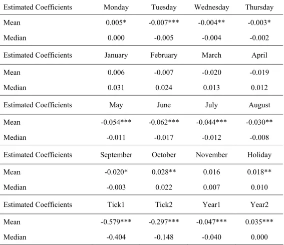
Following Chordia, Sarkar, and Subrahmanyam (2005), we regress stock i’s QSPR on day s on a set of variables known to capture seasonal variation in liquidity:
, 2 1 2 1 3, 4, 5, , , 2 , 1 11 1 , , 4 1 , , , s i s i s i s i s i s i k s k k i k s k k i s i ASPR YEAR f YEAR f TICK f TICK f HOLIDAY f MONTH e DAY d QSPR + + + + + + + =
∑
∑
= = (1)In equation (1), the following variables are employed: (i) day of the week dummies (DAYk,s) for Monday through Thursday; (ii) month dummies (MONTHk,s) for January
through November; (iii) a dummy for trading days around holidays (HOLIDAYs); (iv) tick
change dummies TICK1s and TICK2s to capture the tick change from 1/8 to 1/16 on
06/24/1997 and the change from 1/16 to the decimal system on 01/29/2001, respectively; and (v) time trend variables YEAR1s (YEAR2s), equal to the difference between the
current calendar year and 1988 (1997) or the first year when stock i started trading on NYSE, whichever is later. The regression residuals, including the intercept, give the adjusted proportional quoted spread (ASPR). The time-series regression equation is estimated for each stock in our sample.
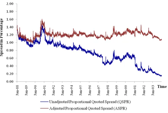
In results reported in the Internet Appendix, the cross-sectional average of the estimated parameters show seasonal patterns in the quoted spread: the bid-ask spreads are typically higher on Fridays and around holidays, and spreads are lower from May to September relative to other months. The tick-size change dummies also pick up a significant decrease in spreads after the change in tick rule on NYSE. These results comport well with the seasonality in liquidity documented in Chordia, Sarkar, and Subrahmanyam (2005). After adjusting for the seasonality in spreads, we do not observe any significant time trend. In Table I, the unadjusted spread (QSPR) exhibits a clear time trend with the annual average spread decreasing from 1.26% in 1988 to 0.26% in 2003, but the trend is removed in the time series of the seasonally adjusted spread (ASPR) annual averages. When plotting the two series, QSPR and ASPR, in Figure 1, we find that our adjustment process does a reasonable job in controlling for the deterministic time-series trend in stock spreads.
[Insert Table I and Figure 1 about here] II. Liquidity and Past Returns
A. Time-series Analysis
We start our analyses by first aggregating the daily adjusted spreads for each stock to obtain average weekly spreads. Denoting firm i’s adjusted proportional spread in week t as ASPRi,t, we perform our analysis on changes in weekly spreads, (ASPRi,t minus
ASPRi,t-1 ) or ΔASPRi,t.7 We regress ΔASPRi,t on the lagged market return (Rm,t-1), proxied
by the CRSP value-weighted index. Since the exact horizon over which declines in aggregate asset values affect liquidity is an empirical question, we examine the effect of up to four lags of weekly returns.8 We test the key prediction of the underlying
theoretical models that liquidity is affected by lagged market returns, particularly, negative returns. At the same time, it is possible that changes in liquidity are affected by lagged firm-specific returns, since large changes in firm value may have similar wealth effects. Firm i’s idiosyncratic returns (Ri,t) are defined as the difference between week t
returns on stock i and the market index.9
We introduce a set of firm-specific variables to control for other sources of intertemporal variation in liquidity. Market microstructure models in Demsetz (1968), Stoll (1978), and Ho and Stoll (1980) suggest that high volumes reduce inventory risk per trade and thus should lead to smaller spreads. We add weekly changes in turnover (ΔTURNit), measured by total trading volume divided by shares outstanding for firm i, to
control for the spread changes arising from the market maker’s inventory concerns. Chordia, Roll, and Subrahmanyam (2002) report that order imbalances are correlated with spreads and conjecture that this could arise because of the market maker’s difficulty in adjusting quotes during periods of large order imbalances. To control for this effect, we add changes in the relative order imbalance (ΔROIBit), measured by the change in
absolute value of the weekly difference in the dollar amount of buyer- and seller-initiated orders standardized by the dollar amount of trading volume over the same period.
It is well known that bid-ask spreads are positively affected by return volatility due to higher adverse selection and inventory risk (see, for example, Stoll (1978)). In the volatility-return literature, a drop in stock prices increases financial leverage, which makes the stock riskier and increases its subsequent volatility (see Black (1976) and Christie (1982)). This implies that negative returns may increase spreads through their impact on subsequent volatility. In Vayanos (2004), variation in demand for liquidity is
driven by changes in market volatility and during volatile periods increased risk aversion leads to a flight to quality (here transactions costs are fixed over time). Vayanos (2004) suggests that if transaction costs are higher during volatile times, the impact of volatility on liquidity (premia) would be even stronger, emphasizing an important connection between changes in market volatility and liquidity. We account for these volatility effects by including contemporaneous and lagged changes in weekly volatility of market returns (ΔSTDm,t) and volatility of stock i returns (ΔSTDi,t). Weekly volatility estimates are
obtained from daily returns over the previous four weeks using the method described in French, Schwert, and Stambaugh (1987). Finally, we add lagged changes in spreads to account for any serial correlations.
Weekly changes in adjusted spreads for each firm are regressed on weekly variables as defined above: , , 4 1 , , 1 , , 6 1 , 5 1 , 4 1 , 3 , 2 , 1 4 1 , , 4 1 , , , t i k ik it k t i i t i i t i i t m i t i i t m i k ik it k k ik mt k i t i ASPR ROIB c TURN c STD c STD c STD c STD c R R ASPR ε φ γ β α + Δ + Δ + Δ + Δ + Δ + Δ + Δ + + + = Δ
∑
∑
∑
= − − − − − = − = − (2)We run the time-series regression in equation (2) for each stock and report the mean and median of the estimated regression coefficients across all firms in our sample, taking into account the cross-equation correlations in the estimated parameters in computing the standard errors.10 Table II presents the equally weighted average coefficients. Consistent with previous literature, we find that a decrease in turnover or an increase in market and idiosyncratic volatility predict higher spreads. Further, spreads increase when there is an increase in contemporaneous or lagged volatility. The coefficient associated with changes in order imbalance (ΔROIBit), on the other hand, has a positive value as expected, but is
More importantly, we find that the lagged market returns in each of the past four weeks affect current changes in spreads, with the effects declining rapidly as we move to longer lags. Additionally, lagged idiosyncratic returns have a monotonically decreasing and significant relation with current changes in adjusted spreads. Thus, consistent with the theoretical predictions in Kyle and Xiong (2001), Brunnermeier and Pedersen (2009), Garleanu and Pedersen (2007), and others, the wealth effect of a market wide drop in asset prices is associated with a fall in liquidity.11
The models that link changes in market prices and liquidity actually pose a stronger prediction: the relation should be stronger for prior losses than gains. Accordingly, we modify equation (2) to allow spreads to react differentially to positive and negative lagged returns: , , 4 1 , , 1 , , 6 1 , 5 1 , 4 1 , 3 , 2 , 1 4 1 ,, , ,, 4 1 , , 4 1 ,, , , , 4 1 , , , t i k ik it k t i i t i i t i i t m i t i i t m i k DOWN ik it k DOWN it k k ik it k k DOWN ik mt k DOWN mt k k ik mt k i t i ASPR ROIB c TURN c STD c STD c STD c STD c D R R D R R ASPR ε φ γ γ β β α + Δ + Δ + Δ + Δ + Δ + Δ + Δ + + + + + = Δ
∑
∑
∑
∑
∑
= − − − − − = − − = − = − − = − (3)where DDOWN,m,t (DDOWN,i,t ) is a dummy variable that is equal to one if and only if Rm,t
(Ri,t) is less than zero. The control variables are identical to those defined in equation (2).
In Panel B of Table II, we find a significantly greater effect of negative market returns on liquidity: the regression coefficient on lagged market returns in week t-1 rises significantly from -0.413 to -1.223 when the market return is negative. Spreads are also asymmetrically related to lagged idiosyncratic returns, although the magnitude of the asymmetry is less dramatic, with the regression coefficient changing from -0.473 to -0.631. Interestingly, the sharp increase in spreads in week t-1, due to negative market
returns, reverses to its mean in weeks t-3 and t-4, indicating that the liquidity effects last up to two weeks.
[Insert Table II about here]
To examine whether the magnitude of lagged returns has any material impact on liquidity, the regression specification is
, , 4 1 , , 1 , , 6 1 , 5 1 , 4 1 , 3 , 2 , 1 4 1 ,, , ,, 4 1 ,, , ,, 4 1 , , 4 1 ,, , , , 4 1 ,, , , , 4 1 , , , t i k ik it k t i i t i i t i i t m i t i i t m i k UP LARGE ik it k UP LARGE it k k DOWN LARGE ik it k DOWN LARGE it k
k ik it k k UP LARGE ik mt k UP LARGE mt k
k DOWN LARGE ik mt k DOWN LARGE mt k k ik mt k i t i ASPR ROIB c TURN c STD c STD c STD c STD c D R D R R D R D R R ASPR ε φ γ γ γ β β β α + Δ + Δ + Δ + Δ + Δ + Δ + Δ + + + + + + + = Δ
∑
∑
∑
∑
∑
∑
∑
= − − − − − = − − = − − = − = − − = − − = − (4)where DDOWN LARGE,m,t (DUP LARGE,m,t ) is a dummy variable that is equal to one if and only
if Rm,t is more than 1.5 standard deviations below (above) its unconditional mean return.
Similarly, DDOWN LARGE,i,t (DUP LARGE,i,t ) is a dummy variable that is equal to one if and
only if Ri,t is more than 1.5 standard deviations below (above) its mean return.12
In Table II, Panel C, large negative market shocks significantly widen the bid-ask spreads while large positive market returns have an insignificant marginal effect, reinforcing the striking asymmetric effect of market returns on liquidity. Our findings add to those in Chordia, Roll, and Subrahmanyam (2001, 2002), who show that at the aggregate level, daily spreads increase dramatically following days with negative market returns but decrease only marginally on positive market daily returns. Consistent with the results in Panel B, the increase in spreads following large negative market returns in week t-1 reverses at longer lags.
(large) negative market return in week t-1, after controlling for other determinants of spreads. Second, Deuskar (2007) presents a model where an increase in investors’ perceived asset risk reduces current prices and makes the market more illiquid. In her model, higher forecasts of volatility affect investor sentiment and hence realized volatility and liquidity. Specifically, her model predicts lowers liquidity when misperceived volatility, measured by the difference between implied volatility of S&P 100 index options (VIX) and realized index volatility, is higher. Consistent with Dueskar (2007), we find that changes in weekly adjusted spread are significantly and positively related to contemporaneous and lagged misperceived weekly volatility. However, the misperceived volatility effects do not displace the strong negative influence of lagged returns.13 Moreover, adding more lags of volatility does not affect our results, indicating that the intertemporal influence of volatility is different from the return effects. Hence, our evidence on lower liquidity following a decrease in aggregate market value of securities is robust.
B. Evidence on the Effects of Funding Constraints
We interpret the relation between market declines and liquidity dry-ups as indicative of capital constraints in the marketplace. A direct test of this supply-side explanation requires that we identify independent changes in funding liquidity at weekly frequencies. Although we do not have access to direct measures of aggregate supply shocks, we use indirect measures from the financial sector to investigate if the contraction in liquidity is consistent with liquidity providers becoming more capital constrained. With equation (3) as a starting point, we examine if the sensitivity of changes in spreads to negative market
returns differs during periods when the suppliers of liquidity are likely to face capital tightness. The following regression model is estimated:
, , 4 1 , , 1 , , 6 1 , 5 1 , 4 1 , 3 , 2 , 1 4 1 ,, , ,, 4 1 , , 1 , 1 , , 1 , , , , 4 1 ,, , , , 4 1 , , , t i k ik it k t i i t i i t i i t m i t i i t m i k DOWN ik it k DOWN it k k ik it k t CAP t m DOWN t m k i CAP DOWN k DOWN ik mt k DOWN mt k k ik mt k i t i ASPR ROIB c TURN c STD c STD c STD c STD c D R R D D R D R R ASPR ε φ γ γ β β β α + Δ + Δ + Δ + Δ + Δ + Δ + Δ + + + + + + = Δ
∑
∑
∑
∑
∑
= − − − − − = − − = − − − − = − − = − (5)where DCAP,t is a dummy variable that takes a value of one only if week t is associated
with periods of higher capital constraints.
We use three proxies to capture tightness of capital in the market. The first proxy is based on the (value-weighted) return on the portfolio of investment banks and securities brokers and dealers listed on NYSE, defined by SIC code 6211.14 We compute the excess returns on the portfolio of stocks in the investment banking sector by the residuals from a one-factor market model regression. A large fall in the market value of the firms operating in investment banking and securities brokerage services is likely to reflect a weak aggregate balance sheet of the funding sector. Hence, when the excess returns on this portfolio of financial intermediaries are negative in week t, DCAP,t is set to one.15
Adrian and Shin (2008) show that the financial intermediaries adjust their leverage in a procyclical manner, with expansion and contraction of their balance sheets effected through repos. For example, when financial intermediaries have weak balance sheets, their leverage is too high. The ensuing capital shortage forces the intermediaries to contract their balance sheets.16 Adrian and Shin show that these changes in aggregate intermediary balance sheets are linked to funding liquidity through shifts in market wide risk appetite. We therefore use the weekly changes in aggregate repos as our second
measure of constraints in the funding market and set DCAP,t to one when there is a decline
in aggregate repos in week t.17
Our third measure of funding liquidity relies on the weekly spread in commercial paper (CP), measured as the difference in the weekly returns on the three-month commercial paper rate and three-month Treasury bill rate.18 It is well known that the CP market is very illiquid. As Krishnamurthy (2002) shows, the difference in the return on CP and T-bills (or the CP spread) reflects a liquidity premium demanded by the large investors in CP such as money market mutual funds and other financial corporations. Gatev and Strahan (2006) use the CP spread to measure liquidity supply and show that the spread widens during liquidity events. Since changes in CP spreads are related to the willingness of these intermediaries to provide liquidity, we argue that an increase in the weekly CP spread is likely to be associated with a period when the funding market is capital constrained. Hence, DCAP,t is equal to one when there is an increase in the CP
spread in week t.
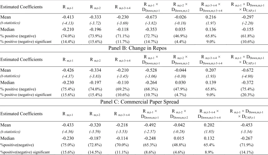
Panel A of Table III shows that a decline in aggregate market valuations leads to a significantly greater increase in bid-ask spreads when there is also an underperformance in the investment banking and brokerage sector.19 In Panel B, a contraction in the balance sheet of the financial intermediaries, measured by a decrease in repos, has a similar effect. To be precise, a negative return on the market index in week t-1 lowers the regression coefficient for market returns from -0.43 to -0.95. A simultaneous decrease in aggregate repos in the capital markets magnifies the impact of negative market returns to -1.63. Finally, our findings are reinforced by a similar amplification of the effect of negative market returns in Panel C, following an increase in CP spreads. Together, the
evidence in Table III is strongly supportive of our interpretation that liquidity dry-ups following market declines are related to tightness in funding liquidity.
[Insert Table III about here]
C. Cross-sectional Evidence
The theoretical models in Brunnermeier and Pedersen (2009) and Garleanu and Pedersen (2007) suggest that high volatility stocks require greater use of risk capital and are more likely to suffer higher haircuts (margin requirements) when funding constraints bind. Consequently, a drop in funding liquidity (large negative market return shock) increases the differential liquidity between high and low volatility securities.
In this subsection, we examine the cross-sectional differences in the relation between lagged returns and spreads among stocks that differ in volatility, controlling for firm size. Firms are sorted into nine size-volatility portfolios based on two-way dependent sorts on each firm’s beginning-of-year market capitalization and its return volatility in the previous year, and the portfolio composition is rebalanced each year. In each week t, we average the adjusted spreads on each firm to produce nine portfolio-level spreads, ASPRp,t. Similar to the firm-specific variables defined in equation (3), for each week t, we
average the relative order imbalance across all firms in each portfolio, denoted as ROIBp,t,
and calculate portfolio turnover, TURNp,t, portfolio-specific returns (Rp,t) and volatility,
STDp,t. We regress the change in spreads at the portfolio level on changes in the control
variables as well as portfolio and market returns, analogous to equation (3), but for portfolio p, where p=1,2,…,9:
, , 4 1 , , 1 , , 6 1 , 5 1 , 4 1 , 3 , 2 , 1 4 1 , , , , , 4 1 , , 4 1 , , , , , 4 1 , , , t p k pk pt k t p p t p p t p p t m p t p p t m p k DOWN pk pt k DOWN pt k k pk pt k k DOWN pk mt k DOWN mt k k pk mt k i t p ASPR ROIB c TURN c STD c STD c STD c STD c D R R D R R ASPR ε φ γ γ β β α + Δ + Δ + Δ + Δ + Δ + Δ + Δ + + + + + = Δ
∑
∑
∑
∑
∑
= − − − − − = − − = − = − − = − (6)The system of equations in (6) is estimated using the seemingly unrelated regression (SUR) method, allowing for cross-equation correlations. Consistent with the results in Table II, Table IV shows that changes in spreads are negatively related to market returns, controlling for portfolio-specific factors. The sensitivity of spreads to market returns is larger for high volatility portfolios, particularly during market downturns. These sharp increases in spreads reverse in subsequent weeks, revealing the short-run nature of the phenomenon. Our results are not a manifestation of size-related effects since we find analogous results within each of the size thirtiles. The reaction of spreads to own- portfolio negative returns are less dramatic, however. Hence, less liquidity is available for high volatility stocks when the liquidation of these assets (collateral) becomes more costly, consistent with a flight to liquidity.
[Insert Table IV about here]
It is interesting to note that the impact of negative market returns on liquidity is in the same direction for each of the nine size-volatility portfolios, suggesting a high commonality in liquidity, an issue that we investigate further in the next section.
III. Commonality in Liquidity
A. Commonality in Liquidity and Market Returns
When market makers and other intermediaries are constrained by their capital base, a large negative return reduces the pool of capital that is tied to marketable securities and
hence reduces the supply of liquidity. The theoretical model in Brunnermeier and Pedersen (2009), for example, predicts that the funding liquidity constraints increase the commonality in liquidity across securities. In a recent paper, Kamara, Lou, and Sadka (2008) find that liquidity betas change over time and that these changes are affected by market volatility as well as market returns.
We start with an investigation of the impact of market returns on a firm’s liquidity beta, using the regression framework in (3). We do this by introducing a measure of weekly market adjusted spreads, ASPRm,t, which is obtained by averaging the firm-level
adjusted spreads, (
∑
iN=1ASPRi,t)/N. The weekly change in market spreads (ASPRm,t-ASPRm,t-1) is denoted as ΔASPRm,t and the sensitivity of firm i’s spread to ΔASPRm,t is its
liquidity beta, bLIQ,i.
t i k ik it k t i i t i i t i i t m i t i i t m i k DOWN ik it k DOWN it k k ik it k k DOWN ik mt k DOWN mt k k ik mt k t m DOWN t m i DOWN LIQ t m i LIQ i t i ASPR ROIB c TURN c STD c STD c STD c STD c D R R D R R D ASPR b ASPR b ASPR , 4 1 , , 1 , , 6 1 , 5 1 , 4 1 , 3 , 2 , 1 4 1 ,, , ,, 4 1 , , 4 1 ,, , , , 4 1 , , , , , , , , , , ε φ γ γ β β α + Δ + Δ + Δ + Δ + Δ + Δ + Δ + + + + + Δ + Δ + = Δ
∑
∑
∑
∑
∑
= − − − − − = − − = − = − − = − (7) . , 4 1 , , 1 , , 6 1 , 5 1 , 4 1 , 3 , 2 , 1 4 1 ,, , ,, 4 1 , , 4 1 ,, , , , 4 1 , , , , , , , , , , , , , , , t i k ik it k t i i t i i t i i t m i t i i t m i k DOWN ik it k DOWN it k k ik it k k DOWN ik mt k DOWN mt k k ik mt k t m LARGE DOWN t m i LARGE DOWN LIQ t m SMALL DOWN t m i SMALL DOWN LIQ t m i LIQ i t i ASPR ROIB c TURN c STD c STD c STD c STD c D R R D R R D ASPR b D ASPR b ASPR b ASPR ε φ γ γ β β α + Δ + Δ + Δ + Δ + Δ + Δ + Δ + + + + + Δ + Δ + Δ + = Δ∑
∑
∑
∑
∑
= − − − − − = − − = − = − − = − (8)It should be noted that we exclude firm i in the computation of market spreads. Although changes in liquidity levels are different from liquidity commonality, it is possible that they are correlated. For example, if low market returns predict low liquidity
for all stocks, then liquidity covariance with aggregate liquidity may increase following low market returns. Hence, we test for both liquidity level and commonality effects in equation (7). Specifically, we examine whether bLIQ,i changes during periods of negative
market returns, as captured by bLIQ,DOWN,i . In equation (8) we also investigate whether
bLIQ,i changes when market returns are negative and small (bLIQ,DOWN,SMALL,i) or negative
and large (bLIQ,DOWN,LARGE,i), where small (large) is defined as negative market returns that
are less (more) than 1.5 standard deviations below the unconditional mean market returns.
Consistent with the findings in Kamara, Lou, and Sadka (2008), Panel A of Table V shows that bLIQ,i increases significantly from 0.56 to 0.87 in down market states. In Panel
B, the largest increase in liquidity commonality happens during large market downturns, when bLIQ,i increases to 0.95. Moreover, the asymmetric effect of market returns on
spreads documented in Section II persists after accounting for changes in liquidity commonality. Hence, the results in Table V emphasize two separate effects: an increase in illiquidity levels as well as commonality in response to market downturns.
[Insert Table V about here]
We also investigate the effect of market returns on commonality in liquidity using an alternate metric that captures comovement. The R2 statistic from the market model regression has been extensively used to measure comovement in stock prices (e.g., Roll (1988), Morck, Yueng, and Yu (2000)). We follow Chordia, Roll, and Subrahmanyam (2000) and use a single-factor market model to compute the commonality in liquidity. Changes in daily adjusted proportional spreads for firm i on day s (ΔASPRi,s) are
. , , , ,s i LIQi ms is i a b ASPR ASPR = + Δ +ε Δ (9)
For each stock i with at least 15 valid daily observations in month t, the market model regression yields a regression R2 denoted as R2i,t. A high R2i,t indicates that a large portion
of the variation in liquidity for stock i in month t is due to common, market wide liquidity movements. For each month t, the strength of liquidity commonality is measured by taking an equally weighted average of R2i,t, denoted as R2t.
Figure 2 shows significant time-series variation in liquidity commonality, R2t, over
the sample period 1988 to 2003. We observe spikes in liquidity commonality associated with periods of liquidity crisis. For example, the highest levels of commonality in liquidity in Figure 2 coincide with liquidity dry-ups during the Asian financial crisis (1997), LTCM crisis (1998), and September 11, 2001 terrorist attacks. These periods are also accompanied by large negative market returns, highlighting the episodic nature of illiquidity. The average liquidity R2 increases to 10.1% in large negative market returns states, compared to 7.4% when market returns are positive. In results available in the Internet Appendix, the dynamic conditional correlations (DCC) methodology introduced by Engle (2002) yields supportive findings: the conditional correlations in illiquidity (spreads) among size-sorted portfolios are significantly higher following large market declines. We also find a similar increase in the conditional correlation between two portfolios of stocks constructed based on whether the stock is an S&P 500 index stock or not. The latter result suggests that the common variation in liquidity cannot be fully explained by demand for liquidity by index-linked funds or index arbitrageurs (see
Harford and Kaul (2005)). Our results underscore the main idea that illiquidity becomes more correlated across all assets following market declines.
[Insert Figure 2 about here]
The intertemporal variation in liquidity commonality may also be affected by factors related to changes in demand for liquidity. In Vayanos (2004), investors become more risk averse and their preference for liquidity increases in volatile times. Consequently, a jump in market volatility, the main state variable in his model, is associated with higher demand for liquidity and conceivably increases liquidity commonality. Extreme aggregate imbalances in the buyer- and seller-initiated orders for securities may increase the demand for liquidity as shown by Chordia, Roll, and Subrahmnayam (2002). If high levels of aggregate order imbalance impose similar pressure across securities, they are also likely to increase commonality in spreads. In addition, correlated shifts in demand by buyer- or seller-initiated trades would lead to commonality in order imbalances. Hence, we explore the impact of both the level and commonality in order imbalances on liquidity commonality. The level of order imbalances (ROIB) is defined above in Section II. To measure commonality in order imbalances (ROIBCOM), we estimate the R2 from a
regression of individual firm order imbalances on market (equally weighted average) order imbalances, similar in spirit to the liquidity commonality measure using proportional spreads in equation (9).
We introduce these additional variables that may affect liquidity commonality within a regression framework. Since the R2
t values are constrained to be between zero and one
by construction, we define liquidity comovement as the logit transformation of R2t,
as well as market returns (Rmt), taking into account the sign and magnitude of market returns: , 3 2 , 1 , , , , , t t t t m t LARGE UP t m LARGE UP t LARGE DOWN t m LARGE DOWN t m t ROIBCOM c ROIB c STD c D R D R R a LIQCOM ε β β β + + + + + + + = (10)
where the return and dummy variables are defined in equation (4).
As shown in Table VI, liquidity comovement is strongest when there is a large drop in aggregate market prices. Shifts in the order imbalance comovement, which we interpret as a measure of correlation in demand for liquidity, are positively associated with liquidity commonality. The level of aggregate order imbalance (ROIB) also positively affects liquidity commonality. Consistent with the prediction in Vayonas (2004), uncertainty in the market (STDm,t) increases investor demand for liquidity and
subsequently increases liquidity commonality. Nevertheless, adding these measures of demand effects does not eliminate the significant asymmetric effect of market returns on liquidity commonality.
To the extent that comovement in order imbalances across securities picks up correlation in demand for liquidity, it would be interesting to document the sources that drive the common variations in order flow. We consider one more explanatory variable: monthly net flow of funds into U.S. equity mutual funds for our sample period from 1988 to 2003. We divide the net fund flow data from Investment Company Institute by the total assets under management by U.S. equity funds to generate our monthly time series of net mutual fund flow. When there is a large withdrawal of money by mutual fund owners in aggregate, fund managers are less willing and able to hold (particularly illiquid) assets, creating correlated demand for liquidity across stocks.
As reported in column (4) of Table VI, order imbalance comovement increases with market volatility and is negatively related to net mutual fund flows, corresponding to changes in demand for liquidity. Unlike the evidence on liquidity commonality, order imbalances across stocks decrease after a large decline in market valuations. The latter result is not surprising since market returns and constraints on aggregate capital are not expected to affect liquidity demand in the same way.
[Insert Table VI about here]
The positive correlation between the two comovement measures suggests that these variables may affect each other simultaneously. To address this endogeneity problem, we re-estimate the coefficients based on two-stage least squares (2SLS) estimation, using net mutual fund flow and lagged order imbalance comovement to identify the demand (commonality in order imbalance) equation. As shown in the last two columns of Table VI, our finding that liquidity commonality increases in large down market states is robust.
Overall, the results show that while liquidity commonality is driven by changes in supply as well as demand for liquidity, the demand factors cannot explain the asymmetric effect of market returns on liquidity. On the other hand, the increase in liquidity commonality in down market states is consistent with the adverse effects of a decrease in the supply of liquidity.
B. Industry Spillover Effects
Virtually all the theoretical models, including Kyle and Xiong (2001), Gromb and Vayanos (2002), Brunnermeier and Pedersen (2009), and Garnealu and Pedersen (2007),
suggest a contagion in illiquidity. We broaden our investigation by addressing whether industry-wide comovement in liquidity is affected by a decrease in the valuation of stocks from other industries, over and above the effect of own-industry portfolio returns. If commonality in liquidity is driven by capital constraints faced by the market making sector in supplying liquidity, we should observe correlated illiquidity within an industry increase with a decline in the market values of securities in other industries.
We begin by estimating in each month the following industry factor model for daily changes in spreads for security i (ΔASPRi,s):
, , , , ,s i LIQi INDjs is i a b ASPR ASPR = + Δ +ε Δ (11)
where the industry liquidity factor (ΔASPRINDj,s) is the daily change in the equally
weighted average of adjusted spreads across all stocks in industry j on day s. Similar to our approach in equation (9), we average the regression R2 from equation (11) for each month t, across all firms in industry j. To obtain an industry-wide measure of commonality in liquidity for each month t, we perform a logit transformation of the industry average R2, denoted as LIQCOMINDj,t. We form 17 industry-wide comovement
measures using the SIC classification derived by Fama and French, which is provided by Kenneth French’s online data library.20 LIQCOMINDj,t, is regressed on the monthly
returns on the industry portfolio j (RINDj,t) and the returns on the market portfolio,
excluding portfolio j (RMKTj,t), taking into account the sign and magnitude of these
returns: t t MKTj DOWN t MKTj DOWN t MKTj t INDj DOWN t INDj DOWN t INDj t INDj D R R D R R a LIQCOM ε β β δ δ + + + + + = , , , , , , , , , (12)
, , , , , , , , , , , , , , , , t t MKTj LARGE UP t MKTj LARGE UP t MKTj LARGE DOWN t MKTj LARGE DOWN t MKTj t INDj LARGE UP t INDj LARGE UP t INDj LARGE DOWN t INDj LARGE DOWN t INDj t INDj D R D R R D R D R R a LIQCOM ε β β β δ δ δ + + + + + + + = (13)
where the dummy variables are defined in the same way as in equations (3) and (4). The regression coefficient associated with the independent variable RMKTj,t measures liquidity spillover effects.
As presented in Table VII, we find that the returns on the market portfolio (i.e., the portfolio of securities in other industries, excluding own industry) exert a strong influence on comovement in liquidity within the industry, especially when the market returns are negative. In fact, the market portfolio returns dominate the industry returns in terms of the effect on industry-wide liquidity movements. The regression coefficient estimate on negative market returns is a significant -1.995 while the coefficient on negative industry returns is smaller at -0.986. When we separate the returns according to their magnitude, large negative market returns turn out to have the greatest impact on industry-level liquidity movements. In Table VII, we also obtain similar spillover effects of market wide returns when we replace LIQCOMINDj,t with the industry average liquidity
betas, bLIQ,t (defined in equation (11)). These results strongly support the idea that when
large negative market returns occur, spillovers due to capital constraints extend across industries, increasing the commonality in liquidity.
[Insert Table VII about here]
IV. Liquidity and Short-term Price Reversals
In Campbell, Grossman, and Wang (1993), risk-averse market makers require compensation for supplying liquidity to meet fluctuations in aggregate demand for
liquidity. This cost of providing liquidity is reflected in the temporary decrease in prices accompanying heavy sell volume and the subsequent increase as prices revert to fundamental values.21 Conrad, Hameed, and Niden (1994), Avramov, Chordia, and Goyal (2006), and Kaniel, Saar, and Titman (2008) provide empirical support for the relation between short-term price reversals and illiquidity and show that high volume stocks exhibit significant weekly return reversals. According to the collateral-based models discussed earlier, the return reversals should be stronger following market declines.
We examine the extent of price reversals in different market states using two empirical trading strategies, namely, contrarian and limit order trading strategies. The first strategy relies on the formulation in Avramov, Chordia, and Goyal (2006). We construct Wednesday to Tuesday weekly returns for all NYSE stocks in our sample for the period 1988 to 2003. Skipping one day between two consecutive weeks avoids the potential negative serial correlation caused by the bid-ask bounce and other microstructure influences. Next, we sort the stocks in week t into positive and negative return portfolios. For each week t, returns on stock i (Rit) that are higher (lower) than the
median return in the positive (negative) return portfolio are classified as winner (loser) securities. We use stock i’s turnover in week t (Turnit) to measure the amount of trading.
The contrarian portfolio weight of stock i in week t+1 within the winner and loser portfolios is given by + =−
∑
= Npt i it it t i t i t p i R Turn R Turn w 1 , , , , 1 ,, / , where Npt denotes the
number of securities in the loser or winner portfolios in week t. The contrarian investment strategy is long on the loser securities and short on the winner securities. The
contrarian profits for the loser and winner portfolios for week t+k are:
∑
= + + + = Np i i pt it k k t p, 1w, , 1R,π , which can be interpreted as the return to a $1 investment in each portfolio. The zero-investment profits are obtained by taking the difference in profits from the loser and winner portfolios.
We investigate the effect of lagged market returns by conditioning the contrarian profits on cumulative market returns over the previous four weeks. Specifically, we examine contrarian profits in four market states: large up (down) markets defined as market return being more than 1.5 standard deviations above (below) the mean return; and small up (down) markets, defined as market returns between zero and 1.5 (-1.5) standard deviations around the mean return.
In the second trading strategy, we follow Handa and Schwartz (1996) and devise a simple limit order trading rule to measure the profits to supplying liquidity.22 When a limit buy order is submitted below the prevailing bid price, the limit order trader provides liquidity to the market. If price variations are due to short-term selling pressure, the limit buy order will be executed and we should observe subsequent price reversals, reflecting compensation for liquidity provision. At the same time, the limit order trader expects to lose from the trade upon arrival of informed traders, in which case the price drop would be permanent (i.e., a limit buy order imbeds a free put option).
The limit order strategy is implemented as follows. At the beginning of each week t, a limit buy order is placed at x% below the opening price (Po). We consider three values
of x: 3%, 5%, and 7%. If the transaction price falls to Po (1- x%) or below within week t,
2). If the limit order is not executed in week t, we assume that the order is withdrawn. A similar strategy is employed to execute limit sell orders if prices reach or exceed Po (1+
x%). For the week t+1, we construct the cross-sectional average weekly returns (for buy and sell orders), weighting each stock i by its turnover in week t
∑
= + = Npt i it t i t i Turn Turnw, 1 , / 1 , . Again, we investigate whether the payoff to the limit order trading strategy varies across market states.
Table VIII, Panel A reports a significant contrarian profit of 0.58% in week t+1 (t-statistic=5.38) for the full sample period. The contrarian profit declines rapidly and becomes insignificant as we move to longer lags. Since the contrarian profits and price reversals appear to last for at most two weeks, we limit our subsequent analyses to the first two weeks after portfolio formation. Panel B of Table VIII shows that the largest contrarian profit is registered in the period following a large decline in market prices. Week t+1 profits in the large down market increase noticeably to 1.18% compared to profits of between 0.52% and 0.64% in other market states. We find a similar profit pattern in week t+2, although the magnitude falls quickly. It is worth noting that the loser portfolio shows the largest profit (above 1.0% per week) following large negative market returns.
To ascertain whether the difference in loser and winner portfolio returns can be explained by loadings on risk factors, we estimate the alphas from a Fama-French three-factor model. We regress the contrarian profits on market (return on the value-weighted market index), size (difference in returns on small and large market capitalization portfolios), and book-to-market (difference in returns on value and growth portfolios) factors. 23 The risk-adjusted profits in large down markets remain
economically large at 1.16% per week, indicating that these risk factors cannot explain the price reversals. In results available in the Internet Appendix, we find that the contrarian profits jump to 1.73% following periods of high liquidity commonality (as defined in Section III) and large market declines.
[Insert Table VIII about here]
Table IX, Panel A shows that our limit order trading strategy generates significant profits for all three discount values, that is, 3%, 5% and 7%, with weekly buy-minus-sell portfolio returns ranging from 0.37% to 0.97% in the first week. These returns become economically small in magnitude beyond one week. In Panel B, the buy-minus-sell portfolio returns are similar in all the market states, except for large down states. For example, the 5% limit order trading rule generates buy-minus-sell returns of between 0.63% and 0.68% per week in most market states. The striking exception is in large down markets, where the portfolio returns more than double to 1.56%.
[Insert Table IX about here]
Hence, the evidence from both strategies shows that the compensation for supplying liquidity increases in large down markets, indicative of supply effects in equity markets arising from tightness in capital.
V. Conclusion
This paper documents that liquidity responds asymmetrically to changes in asset market values. Consistent with theoretical models emphasizing changes in the supply of liquidity, negative market returns decrease liquidity much more than positive returns increase liquidity, with the effect being strongest for high volatility firms and during times when the market making sector is likely to face capital tightness. We show a drastic
increase in commonality in liquidity after large negative market returns, and peaks in the commonality measure coincide with periods often associated with liquidity crisis. Hence, market declines affect both liquidity level and liquidity commonality. We also document that liquidity commonality within an industry increases significantly when the returns on other industries (excluding the specific industry) are large and negative, suggesting contagion in illiquidity: illiquidity in one industry spills over to other industries.
The contagion in illiquidity and increase in liquidity commonality as aggregate asset values decline provide indirect evidence of a drop in the supply of liquidity affecting all securities. We argue that demand effects, such as buy-sell order imbalances, cannot fully explain our results. Finally, we use the idea that short-term stock price reversals following heavy trading reflect compensation for supplying liquidity and examine whether the cost of liquidity provision varies with large changes in aggregate asset values. We find that, indeed, the cost of providing liquidity is highest in periods with large market declines and high commonality in liquidity. For example, contrarian or limit order trading strategies based on return reversals produce economically significant returns (between 1.18% and 1.56% per week) after a large decline in aggregate market prices. Taken together, our results support a supply effect on liquidity as advocated by Kyle and Xiong (2001), Gromb and Vayanos (2002), Anshuman and Viswanathan (2005), Brunnermeier and Pedersen (2009), Garleanu and Pedersen (2007), and Mitchell, Pedersen, and Pulvino (2007). Further, our empirical results indicate that the illiquidity effect in the equity market lasts between one to two weeks, on average. We interpret our results as suggesting the presence of supply effects even in liquid markets like U.S. equities with capital flowing into the market fairly quickly.
Overall, our paper presents evidence supportive of the collateral view of market liquidity: market liquidity drops after large negative market returns because aggregate collateral of financial intermediaries falls and many asset holders are forced to liquidate, making it difficult to provide liquidity precisely when the market needs it. However, our evidence is indirect. A fruitful avenue for future research would be to investigate the effect of funding constraints using high frequency data on the balance sheet positions held by intermediaries.
REFERENCES
Acharya, Viral V., and Lasse Heje Pedersen, 2005, Asset pricing with liquidity risk, Journal of Financial Economics 77, 375-410.
Adrian, Tobias, and Hyun Song Shin, 2008, Liquidity and leverage, Working paper, Princeton University.
Allen, Franklin, and Douglas Gale, 2005, From cash-in-the-market pricing to financial fragility, Journal of European Economic Association 3, 535-546.
Amihud, Yakov, and Haim Mendelson, 1986, Asset pricing and the bid-ask spread, Journal of Financial Economics 17, 223-249.
Ang, Andrew, and Joe Chen, 2002, Asymmetric correlations in equity portfolios, Journal of Financial Economics 63, 443-494.
Ang, Andrew, Joe Chen, and Yuhang Xing, 2006, Downside risk, Review of Financial Studies 19, 1191-1239.
Anshuman, Ravi and S. Viswanathan, 2005, Costly collateral and liquidity, Working paper, Duke University.
Avramov, Doron, Tarun Chordia, and Amit Goyal, 2006, Liquidity and autocorrelation of individual stock returns, Journal of Finance 61, 2365-2394.
Baker, Malcolm and Jeremy C. Stein, 2004, Market liquidity as a sentiment indicator, Journal of Financial Markets7, 271-299.
Barber, Brad, Terrance Odean, and Ning Zhu, 2008, Do noise traders move markets? Review of Financial Studies, forthcoming.
Bernado, Antonio, and Ivo Welch, 2003, Liquidity and financial market runs, Quarterly Journal of Economics 119, 135-158.
Black, F., 1976, Studies of stock price volatility changes, Proceedings of the 1976 Meetings of the Business and Economics Statistics Section, American Statistical Association, 177-181.
Brunnermeier, Markus and Lasse Pedersen, 2009, Market liquidity and funding liquidity, Review of Financial Studies 22, 2201-2238.
Campbell, John Y., Sanford J. Grossman, and Jiang Wang, 1993, Trading volume and serial correlation in stock returns, Quarterly Journal of Economics, 108, 905-939. Chordia, Tarun, Richard Roll, and Avanidhar Subrahmanyam, 2000, Commonality in
Chordia, Tarun, Richard Roll, and Avanidhar Subrahmanyam, 2001, Market liquidity and trading activity, Journal of Finance 56, 501-530.
Chordia, Tarun, Richard Roll, and Avanidhar Subrahmanyam, 2002, Order imbalance, liquidity and market returns, Journal of Financial Economics 65, 111-130.
Chordia, Tarun, Asani Sarkar, and Avanidhar Subrahmanyam, 2005, An empirical analysis of stock and bond market liquidity, Review of Financial Studies 18, 85-129. Christie, Andrew A., 1982, The stochastic behavior of common stock variances: Value,
leverage and interest rate effect, Journal of Financial Economics 10, 407-432. Comerton-Forde, Carole, Terence Hendershott, Charles Jones, Pamela Moulton, and
Mark Seasholes, 2008, Time variation in liquidity: The role of market maker inventories and revenues, Working paper, UC-Berkeley.
Conrad, Jennifer, Allaudeen Hameed, and Cathy Niden, 1994, Volume and
autocovariances in short-horizon individual security returns, Journal of Finance 49, 1305-1329.
Coughenour, Jay, and Mohsen Saad, 2004, Common market makers and commonality in liquidity, Journal of Financial Economics 73, 37-69.
Demsetz, Harold, 1968, The cost of transaction, Quarterly Journal of Economics 82, 33-53.
Dueskar, Prachi, 2007, Extrapolative expectations: Implications for volatility and liquidity, Working paper, University of Illinois at Urbana-Champaign.
Eisfeldt, Andrea, 2004, Endogenous liquidity in asset markets, Journal of Finance 59, 1-30.
Engle, Robert, 2002, Dynamic conditional correlation: A simple class of multivariate generalized autoregressive conditional heteroskedasticity models, Journal of Business & Economic Statistics 20, 339-350.
Fama, Eugene F. and Kenneth R. French, 1993, Common risk factors in the return on stocks and bonds, Journal of Financial Economics 33, 3-56.
French, Kenneth, G. William Schwert, and Robert Stambaugh, 1987, Expected stock returns and volatility, Journal of Financial Economics 19, 3-29.
Garleanu, Nicolae, and Lasse Heje Pedersen, 2007, Liquidity and Risk Management, American Economic Review 97, 193-197.
Gatev, Evan, and Philip E. Strahan, 2006, Banks Advantage in Hedging Liquidity Risk: Theory and Evidence from the Commercial Paper Market, Journal of Finance 61, 867-892
Gervais, Simon, and Terrance Odean, 2001, Learning to be Overconfident, Review of Financial Studies 14, 1-27.
Gromb, Denis, and Dimitri Vayanos, 2002, Equilibrium and Welfare in Markets with Financially Constraint Arbitrageurs, Journal of Financial Economics 66, 361-407. Handa, Puneet, and Robert A. Schwartz, 1996, Limit order trading, Journal of Finance
51, 1835-1861.
Harford, Jarrad, and Aditya Kaul, 2005, Correlated Order Flow: Persvasiveness, Sources and Pricing Effects, Journal of Financial and Quantitative Analysis 40, 29-55. Hasbrouck, Joel, and Duane J. Seppi, 2001, Common factors in prices, order flows, and
liquidity, Journal of Financial Economics 59, 383-411.
Ho, Thomas, and Hans H. Stoll, 1980, On dealer markets under competition, Journal of Finance 35, 259-267.
Huberman, Gur, and Dominika Halka, 2001, Systematic liquidity, Journal of Financial Research 24, 161-178.
Kamara, Avi, Xiaoxia Lou, and Ronnie Sadka, 2008, The divergence of liquidity commonality in the cross-section of stocks, Journal of Financial Economics 89, 444-466.
Kaniel, Ron, Gideon Saar, and Sheridan Titman, 2008, Individual investor trading and stock returns, Journal of Finance 63, 273-310.
Karolyi, G. Andrew, Kuan-Hui Lee, and Mathijs A. Van Dijk, 2008, Commonality in returns, liquidity and trading volume around the world, Working paper, Ohio State University.
Kiyotaki, Nobuhiro, and John Moore, 1997, Credit cycles, Journal of Political Economy, 105, 211-248.
Krishnamurthy, Arvind, 2002, The bond/old bond spread, Journal of Financial Economics 66, 463-506.
Kyle, Pete, and Wei Xiong, 2001, Contagion as a wealth effect, Journal of Finance 4, 1401-1440.
Lee, Charles M.C, 1992, Earnings news and small traders: An intraday analysis. Journal of Accounting and Economics 15, 265-302.
Lee, Charles M. C., and Balakrishna Radhakrishna, 2000, Inferring investor behavior: Evidence from TORQ data, Journal of Financial Markets 3, 83-111.
Lee, Charles M. C., and Mark J. Ready, 1991, Inferring trade direction from intraday data, Journal of Finance 46, 733-746.
Mitchell, Mark, Lasse Heje Pedersen, and Todd Pulvino, 2007, Slow moving capital, American Economic Review 97, 215-220.
Morck, Randall, Bernard Yeung, and Wayne Yu, 2000, The information content of stock markets: Why do emerging markets have synchronous stock price movements? Journal of Financial Economics 59, 215-260.
Morris, Stephen, and Hyun Song Shin, 2004, Liquidity black holes, Review of Finance 8, 1-18.
Naik, Narayan, and Pradeep Yadav, 2003, Risk management with derivatives by dealers and market quality in government bond markets, Journal of Finance 5, 1873-1904. Roll, Richard, 1988, R2, Journal of Finance 42, 541-566.
Pastor, Lubos, and Robert F. Stambaugh, 2003, Liquidity risk and