Semi-Parametric Estimators
by
Tchilabalo Abozou Kpanzou
Dissertation presented for the degree of
Doctor of Philosophy at the
Stellenbosch University
Promotor: Prof Tertius de Wet
Co-Promotor: Dr Ariane Neethling
Declaration
By submitting this dissertation electronically, I declare that the entirety of the work contained therein is my own, original work, that I am the sole author thereof (save to the extent explicitly otherwise stated), that reproduction and publication thereof by Stellenbosch University will not infringe any third party rights and that I have not previously in its entirety or in part submitted it for obtaining any qualification.
18 October 2011 Signature: - - - Date:
-TA Kpanzou
Copyright©2011 Stellenbosch University All rights reserved.
Abstract
Measures of inequality, also used as measures of concentration or diversity, are very popular in eco-nomics and especially in measuring the inequality in income or wealth within a population and between populations. However, they have applications in many other fields, e.g. in ecology, linguistics, socio-logy, demography, epidemiology and information science.
A large number of measures have been proposed to measure inequality. Examples include the Gini index, the generalized entropy, the Atkinson and the quintile share ratio measures. Inequality measures are inherently dependent on the tails of the population (underlying distribution) and therefore their estimators are typically sensitive to data from these tails (nonrobust). For example, income distributions often exhibit a long tail to the right, leading to the frequent occurrence of large values in samples. Since the usual estimators are based on the empirical distribution function, they are usually nonrobust to such large values. Furthermore, heavy-tailed distributions often occur in real life data sets, remedial action therefore needs to be taken in such cases.
The remedial action can be either a trimming of the extreme data or a modification of the (traditional) estimator to make it more robust to extreme observations. In this thesis we follow the second option, modifying the traditional empirical distribution function as estimator to make it more robust. Using re-sults from extreme value theory, we develop more reliable distribution estimators in a semi-parametric setting. These new estimators of the distribution then form the basis for more robust estimators of the measures of inequality. These estimators are developed for the four most popular classes of mea-sures, viz. Gini, generalized entropy, Atkinson and quintile share ratio. Properties of such estimators are studied especially via simulation. Using limiting distribution theory and the bootstrap methodology, approximate confidence intervals were derived. Through the various simulation studies, the proposed estimators are compared to the standard ones in terms of mean squared error, relative impact of con-tamination, confidence interval length and coverage probability. In these studies the semi-parametric methods show a clear improvement over the standard ones. The theoretical properties of the quintile share ratio have not been studied much. Consequently, we also derive its influence function as well as the limiting normal distribution of its nonparametric estimator. These results have not previously been published.
In order to illustrate the methods developed, we apply them to a number of real life data sets. Using such data sets, we show how the methods can be used in practice for inference. In order to choose between the candidate parametric distributions, use is made of a measure of sample representative-ness from the literature. These illustrations show that the proposed methods can be used to reach satisfactory conclusions in real life problems.
Opsomming
Maatstawwe van ongelykheid, wat ook gebruik word as maatstawwe van konsentrasie of diversiteit, is baie populêr in ekonomie en veral vir die kwantifisering van ongelykheid in inkomste of welvaart binne ’n populasie en tussen populasies. Hulle het egter ook toepassings in baie ander dissiplines, byvoorbeeld ekologie, linguistiek, sosiologie, demografie, epidemiologie en inligtingskunde.
Daar bestaan reeds verskeie maatstawwe vir die meet van ongelykheid. Voorbeelde sluit in die Gini indeks, die veralgemeende entropie maatstaf, die Atkinson maatstaf en die kwintiel aandeel verhoud-ing. Maatstawwe van ongelykheid is inherent afhanklik van die sterte van die populasie (onderliggende verdeling) en beramers daarvoor is tipies dus sensitief vir data uit sodanige sterte (nierobuust). Inkom-ste verdelings het byvoorbeeld dikwels lang regterInkom-sterte, wat kan lei tot die voorkoms van groot waardes in steekproewe. Die tradisionele beramers is gebaseer op die empiriese verdelingsfunksie, en hulle is gewoonlik dus nierobuust teenoor sodanige groot waardes nie. Aangesien swaarstert verdel-ings dikwels voorkom in werklike data, moet regstellverdel-ings gemaak word in sulke gevalle.
Hierdie regstellings kan bestaan uit of die afknip van ekstreme data of die aanpassing van tradi-sionele beramers om hulle meer robuust te maak teen ekstreme waardes. In hierdie tesis word die tweede opsie gevolg deurdat die tradisionele empiriese verdelingsfunksie as beramer aangepas word om dit meer robuust te maak. Deur gebruik te maak van resultate van ekstreemwaardeteorie, word meer betroubare beramers vir verdelings ontwikkel in ’n semi-parametriese opset. Hierdie nuwe be-ramers van die verdeling vorm dan die basis vir meer robuuste bebe-ramers van maatstawwe van onge-lykheid. Hierdie beramers word ontwikkel vir die vier mees populêre klasse van maatstawwe, naam-lik Gini, veralgemeende entropie, Atkinson en kwintiel aandeel verhouding. Eienskappe van hierdie beramers word bestudeer, veral met behulp van simulasie studies. Benaderde vertrouensintervalle word ontwikkel deur gebruik te maak van limietverdelingsteorie en die skoenlus metodologie. Die voorgestelde beramers word vergelyk met tradisionele beramers deur middel van verskeie simulasie studies. Die vergelyking word gedoen in terme van gemiddelde kwadraat fout, relatiewe impak van kontaminasie, vertrouensinterval lengte en oordekkingswaarskynlikheid. In hierdie studies toon die semi-parametriese metodes ’n duidelike verbetering teenoor die tradisionele metodes. Die kwintiel aandeel verhouding se teoretiese eienskappe het nog nie veel aandag in die literatuur geniet nie. Gevolglik lei ons die invloedfunksie asook die asimptotiese verdeling van die nie-parametriese be-ramer daarvoor af.
Ten einde die metodes wat ontwikkel is te illustreer, word dit toegepas op ’n aantal werklike datastelle. Hierdie toepassings toon hoe die metodes gebruik kan word vir inferensie in die praktyk. ’n Metode in die literatuur vir steekproefverteenwoordiging word voorgestel en gebruik om ’n keuse tussen die kandidaat parametriese verdelings te maak. Hierdie voorbeelde toon dat die voorgestelde metodes met vrug gebruik kan word om bevredigende gevolgtrekkings in die praktyk te maak.
Résumé
Les mesures d’inégalité, également utilisées comme mesures de concentration ou de diversité, sont très populaires dans les sciences économiques, particulièrement en mesurant l’inégalité dans le revenu ou la richesse dans une population et entre des populations. Cependant, elles ont des applications dans beaucoup d’autres domaines, par exemple en écologie, linguistique, sociologie, démographie, épidémiologie et science de l’information.
Un grand nombre de mesures a été proposé pour mesurer l’inégalité. Les exemples incluent l’index de Gini, l’entropie généralisée, la mesure d’Atkinson et le rapport des quintiles du revenu. Les mesures d’inégalité dépendent des queues de la population (distribution fondamentale) et ainsi leurs estima-teurs sont en général sensibles aux données de ces queues (non-robustes). Par exemple, les fonctions de répartition du revenu présentent souvent une longue queue vers la droite, conduisant à l’apparition fréquente de grandes valeurs dans les échantillons. Puisque les estimateurs habituels sont basés sur la distribution empirique, ils sont habituellement non-robustes à de telles grandes valeurs. En outre, les distributions à queue lourde se produisent souvent dans des données de la vie réelle, d’où la nécessité de prendre des mesures correctives dans de tels cas.
L’action corrective peut consister en une coupure délibérée des données extrêmes ou en une modi-fication de l’estimateur (traditionnel) pour le rendre plus robuste aux observations extrêmes. Dans cette thèse nous suivons la deuxième option, modifiant la fonction empirique traditionnelle comme estimateur pour la rendre plus robuste. Utilisant des résultats de la théorie des valeurs extrêmes, nous développons des estimateurs plus fiables de la fonction de répartition dans un cadre semi-paramétrique. Ces nouveaux estimateurs de la fonction de répartition constituent alors la base pour des estimateurs plus robustes des mesures d’inégalité. Ces estimateurs sont développés pour les qua-tre classes les plus populaires des mesures d’inégalité, à savoir Gini, entropie généralisée, Atkinson et rapport des quintiles du revenu. Des propriétés de tels estimateurs sont étudiées par l’intermédiaire de simulations. En utilisant la loi limite et le bootstrap, des intervalles de confiance ont été construits. Par l’intermédiaire de simulations, les estimateurs proposés sont comparés à ceux habituels en termes d’erreur quadratique moyenne, effet relatif de contamination, longueur moyenne d’intervalle de con-fiance et probabilité de couverture. Dans ces études les méthodes semi-paramétriques montrent une amélioration claire par rapport aux méthodes habituelles. Les propriétés théoriques du rapport des quintiles n’ont pas été beaucoup étudiées dans la littérature. Par conséquent, nous dérivons égale-ment sa fonction d’influence aussi bien que la loi normale limite de son estimateur non paramétrique. Ces résultats n’ont pas été précédemment publiés.
Afin d’illustrer les méthodes développées, nous les appliquons à un certain nombre de données réelles. En utilisant de telles données, nous montrons comment ces méthodes peuvent être appliquées dans la pratique pour l’inférence statistique. Afin de choisir entre les distributions paramétriques candi-dates, nous utilisons une mesure de représentativité de l’échantillon proposée dans la littérature. Ces illustrations prouvent que les méthodes proposées sont fiables et peuvent être utilisées pour tirer des
Acknowledgements
• I am very grateful to Prof Tertius de Wet for his guidance and his help throughout this project, patiently supporting and encouraging me, and for thoroughly checking and refining my work. I am also grateful to Dr A Neethling for her support and encouragement.
• I would like to thank Prof M Kidd, Dr TL Berning, Mr JD Van Heerden for providing me with the data.
• I am thankful to the German Academic Exchange Service (DAAD), the African Institute for Mathematical Sciences (AIMS) and Stellenbosch University for providing me with the needed financial support to complete this study.
• I would like to thank my parents for their continued love, support and encouragement throughout the years, and for helping me to keep courageous and strong although I am far from them. The support from all my brothers and sisters is also very much appreciated.
• My special thanks go to my formal lecturers at the University of Lomé, especially Prof KE Gneyou and Prof M Kpékpassi, who made it possible for me to study in South Africa.
• Finally my gratitude goes to all my friends who showed interest in what I have been doing and expressed their care in one way or the other. I particularly think of Antonie Teubes, Isaac Ndlovu, Brigott Bruintjies, Salome Mashilo, Rosette Sifa Vuninga, Reine Hodalo Mbiyou, Ous-man Sawadogo, Joseph Tchérou, Yao Akutor, EmOus-manuel Amouzou, Justin Mabiala, Gaelle Nsoungui, Georges Hemou, Pascal Hemou, Maxime Papouti, Justine Gnama, Eric Saffou, Nom-basa Ntushelo, just to mention some. I sincerely appreciated their support.
Contents
Abbreviations xv
Notation xv
List of Figures xviii
List of Tables xx
1 Introduction 1
1.1 Background and Problem Statement . . . 1
1.2 Scope and Contributions of the Study . . . 3
1.3 Outline of the Study . . . 4
2 Literature Overview 6 2.1 Lorenz Curves . . . 6
2.2 Influence Functions . . . 7
2.3 Inequality Measures: Definitions and Some Properties . . . 8
2.3.1 Generalized Entropy Measures of Inequality . . . 8
2.3.2 Atkinson Class of Inequality Measures . . . 11
2.3.3 Relationship Between the Lorenz Curve and the GE Measures and Between the Lorenz Curve and Atkinson Measures . . . 12
2.3.4 Gini Coefficient . . . 13
2.3.5 Quintile Share Ratio Measure of Inequality . . . 17
2.4 Current Estimation Procedures and Effects of Extreme Values . . . 22
2.4.1 Income Distribution and Inequality Measurement: The Problem of Extreme Values . . . 22
2.4.2 Asymptotic and Bootstrap Inference for Inequality Measures . . . 23
2.4.3 Further Developments on Measures of Inequality . . . 24
3 Heavy Tailed Distributions and Sampling Distributions of the Nonparametric Estimators of Inequality Measures 25 3.1 Heavy Tailed Distributions . . . 26
3.1.1 Pareto distribution . . . 26 3.1.2 Burr Distribution . . . 26 3.1.3 Singh-Maddala Distribution . . . 27 3.1.4 Lognormal Distribution . . . 28 3.1.5 Gamma Distribution . . . 29 3.1.6 Loggamma Distribution . . . 30
3.1.7 Dagum Type I Distribution . . . 30
3.1.8 Fréchet Distribution . . . 31
3.1.9 StudenttDistribution . . . 32
3.2 Sampling Distributions of the Nonparametric Estimators of Inequality Measures . . . . 32
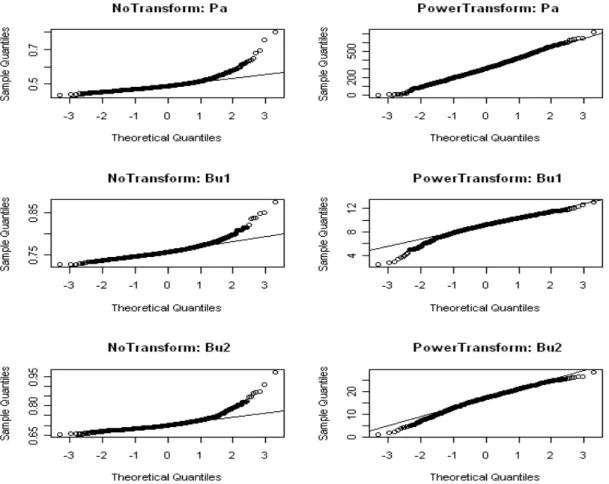
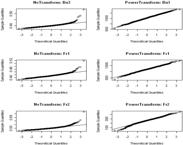
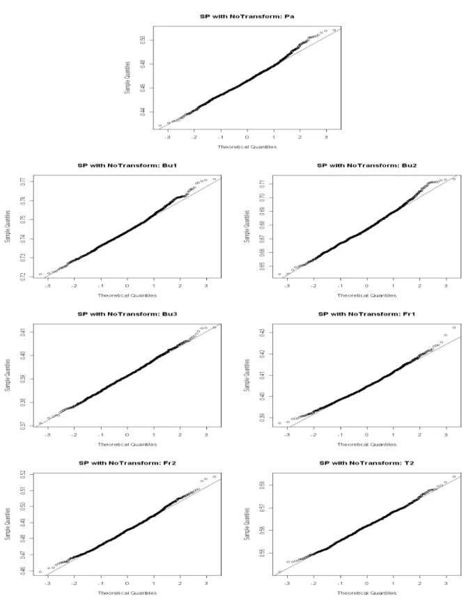
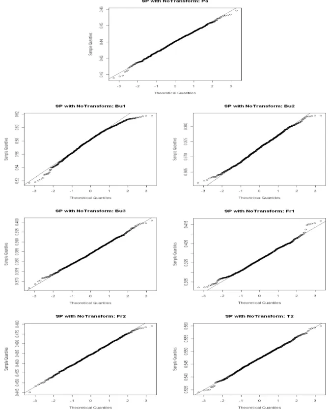
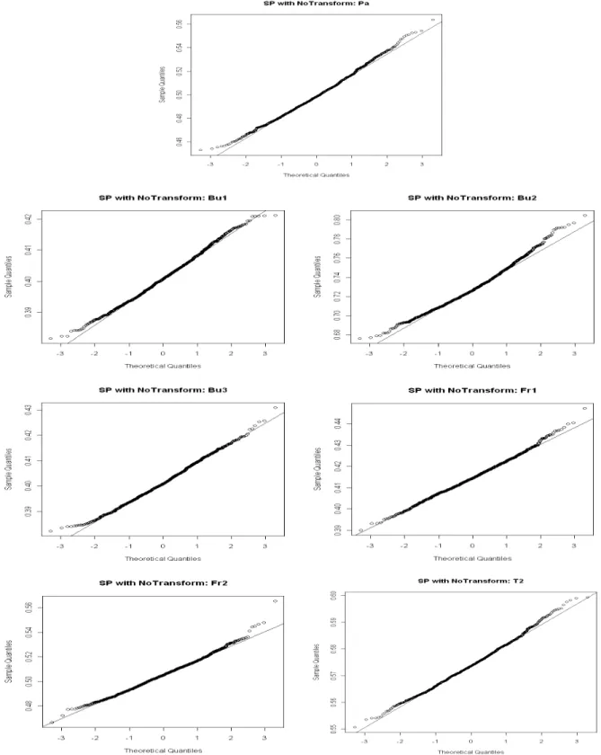
3.2.1 Quantile Plots for the Sampling Distributions . . . 33
3.2.2 Discussion . . . 36
4 Extreme Value Index Estimation and Threshold Selection Methods 37 4.1 Estimators for the Extreme Value Index . . . 38
4.2.1 Integrated Squared Error Estimation . . . 43
4.2.2 Partial Density Component Estimation . . . 44
4.2.3 Minimum Power Divergence Estimation . . . 44
4.3 Threshold Selection Methods . . . 45
4.3.1 Hill Plot Method . . . 45
4.3.2 AltHill Plot Method . . . 46
4.3.3 Guillou and Hall Method . . . 46
4.3.4 Minimum Mean Squared Error Method . . . 47
4.3.5 Drees and Kaufmann Method . . . 47
4.3.6 Hall-Class Method . . . 48
4.3.7 Resampling Method . . . 49
4.3.8 Berning’s Adaptive Methods . . . 50
5 Semi-Parametric Estimation of Inequality Measures 53 5.1 Semi-parametric Estimation of the Underlying Distribution Function . . . 53
5.2 Choices of Parametric Distribution Functions using Extreme Value Theory . . . 56
5.2.1 SP Estimator of the Underlying Distribution when Fitting the GPD . . . 57
5.2.2 SP Estimator of the Underlying Distribution when Fitting the Strict Pareto . . . . 58
5.2.3 SP Estimator of the Underlying Distribution when Fitting the PPD . . . 59
5.3 Semi-Parametric Estimators of Measures of Inequality . . . 60
5.3.1 Semi-Parametric Estimation of Gini Coefficient . . . 60
5.3.2 Semi-Parametric Estimation of Generalized Entropy Inequality Measures . . . . 66
5.3.3 Semi-Parametric Estimation of Atkinson Inequality Measures . . . 73
5.3.4 Semi-Parametric Estimation of Quintile Share Ratio Measure of Inequality . . . 77
6 Confidence Intervals 87
6.1 Some Properties of Confidence Intervals . . . 88
6.2 Confidence Intervals Based on Normal Approximation . . . 89
6.3 Studentt Confidence Intervals . . . 89
6.4 Bootstrap Confidence Intervals . . . 90
6.4.1 Basic Ideas of the Bootstrap . . . 90
6.4.2 Bootstrap Percentile Intervals . . . 92
6.4.3 Bootstrapt Confidence Intervals . . . 93
6.4.4 Bias-Corrected and Accelerated (BCa) Confidence Intervals . . . 94
6.4.5 Semi-Parametric Bootstrap Confidence Intervals . . . 96
6.5 Asymptotic Normality for the Gini, the GE and the Atkinson Measures . . . 97
6.6 Asymptotic Normality for the Quintile Share Ratio . . . 99
7 Simulation Study 101 7.1 Mean Squared Errors and Sensitivity to Contaminations . . . 103
7.1.1 Mean Squared Errors for the Estimators . . . 103
7.1.2 Sensitivity of Inequality Measures to Outliers . . . 105
7.2 Confidence Intervals . . . 107
7.2.1 Simulation Results for Confidence Intervals . . . 109
7.2.2 Discussion of Simulation Results for Confidence Intervals . . . 113
8 Applications 122 8.1 Description of the Data . . . 122
8.2 Estimation of Inequality Measures . . . 125
8.3 Confidence Intervals . . . 126
9 Conclusions and Further Work 138
References 141
Appendix 145
A Outline of Proof of Theorem 6.1 145
B Sampling Distributions for Nonparametric Estimators of Inequality Measures 149
B.1 Generalized Entropy with Parameter 0 (GE0) . . . 150
B.2 Generalized Entropy with Parameter 1 (GE1) . . . 152
B.3 Generalized Entropy with Parameter 1.3 (GE1.3) . . . 154
B.4 Atkinson Coefficient with Parameter 1 (A1) . . . 156
B.5 Atkinson Coefficient with Parameter 1.5 (A1.5) . . . 158
B.6 Atkinson Coefficient with Parameter 2 (A2) . . . 160
C Sampling Distributions for Semi-Parametric Estimators of Inequality Measures 162 C.1 Generalized Entropy with Parameter 0 (GE0) . . . 163
C.2 Generalized Entropy with Parameter 1 (GE1) . . . 166
C.3 Generalized Entropy with Parameter 1.3 (GE1.3) . . . 169
C.4 Atkinson Coefficient with Parameter 1 (A1) . . . 172
C.5 Atkinson Coefficient with Parameter 1.5 (A1.5) . . . 175
C.6 Atkinson Coefficient with Parameter 2 (A2) . . . 178
C.7 Quintile Share Ratio (QSR) . . . 181
D Mean Squared Errors for Estimators of Inequality Measures 184 D.1 Generalized Entropy with Parameter 0 (GE0) . . . 185
D.2 Generalized Entropy with Parameter 1 (GE1) . . . 186
D.4 Atkinson Coefficient with Parameter 1 (A1) . . . 188
D.5 Atkinson Coefficient with Parameter 1.5 (A1.5) . . . 189
D.6 Atkinson Coefficient with Parameter 2 (A2) . . . 190
D.7 Quintile Share Ratio (QSR) . . . 191
E Relative Impact of Contamination for Estimators of Inequality Measures 192 E.1 Generalized Entropy with Parameter 0 (GE0) . . . 193
E.2 Generalized Entropy with Parameter 1 (GE1) . . . 194
E.3 Generalized Entropy with Parameter 1.3 (GE1.3) . . . 195
E.4 Atkinson Coefficient with Parameter 1 (A1) . . . 196
E.5 Atkinson Coefficient with Parameter 1.5 (A1.5) . . . 197
E.6 Atkinson Coefficient with Parameter 2 (A2) . . . 198
E.7 Quintile Share Ratio (QSR) . . . 199
F Properties of Confidence Intervals for Inequality Measures 200 F.1 Generalized Entropy with Parameter 0 (GE0) . . . 201
F.2 Generalized Entropy with Parameter 1 (GE1) . . . 205
F.3 Generalized Entropy with Parameter 1.3 (GE1.3) . . . 209
F.4 Atkinson Coefficient with Parameter 1 (A1) . . . 213
F.5 Atkinson Coefficient with Parameter 1.5 (A1.5) . . . 217
F.6 Atkinson Coefficient with Parameter 2 (A2) . . . 221
F.7 Quintile Share Ratio (QSR) . . . 224
G Standard Errors for the CPs and ACILs 227 G.1 Generalized Entropy with Parameter 0 (GE0) . . . 228
G.2 Generalized Entropy with Parameter 1 (GE1) . . . 230
G.4 Atkinson Coefficient with Parameter 1 (A1) . . . 234
G.5 Atkinson Coefficient with Parameter 1.5 (A1.5) . . . 236
G.6 Atkinson Coefficient with Parameter 2 (A2) . . . 238
Abbreviations
ABias Asymptotic Bias symbolsymbol:
ACIL Average Confidence Interval Length
AMSE Asymptotic Mean Squared Error
AVar Asymptotic Variance
Aν Atkinson measure with parameterν
BCa Bootstrap Calibrated and Accelerated
BCAI BCa interval
BPGPDI Bootstrap percentile interval when using GPD in the tail
BPI Bootstrap percentile interval
BPPI Bootstrap percentile interval when using Pa in the tail
BT GPDI Bootstrapt interval when using GPD in the tail
BT I Bootstrapt interval
BT PI Bootstrapt interval when using Pa in the tail
Bu1 Burr distribution withα=2,τ=0.83andλ=1
Bu2 Burr distribution withα=1,τ=1.4andλ=1
Bu3 Burr distribution withα=0.5,τ=4andλ=1
CI Confidence Interval
CIl Confidence Interval length
CIS Confidence Interval shape
CP Coverage Probability
EV I Extreme Value Index
EV T Extreme Value Theory
Fr1 Frechet distribution withα=2
Fr2 Frechet distribution withα=1.7
GE Generalized Entropy
GEV Generalized Extreme Value
GEν Generalized Entropy measure with parameterν
GPD Generalized Pareto Distribution
IF Influence Function
i.i.d. Independent and identically distributed
MAD Median Absolute Deviation
MCap Market Capitalization
MEF Mean Excess Function
MEP Mean Excess Plot
MLD Mean Logarithmic Deviation
MLE Maximum Likelihood Estimator
MSE Mean Squared Error
NP Nonparametric
Pa Pareto distribution
PDC Partial Density Component
PPD Perturbed Pareto Distribution
PT BCAI Power Transformed bootstrap calibrated and accelerated interval
PT BPI Power Transformed bootstrap percentile interval
QSR Quintile Share Ratio
RIC Relative Impact of Contamination
RIF Relative Influence Function
SE Standard Error
SNI Standard Normal interval
SP Semi-Parametric
SPCo Cowell and Flachaire semi-parametric method
SPGPD Semi-parametric method with GPD in the tail
SPPa Semi-parametric method with strict Pareto in the tail
SPPPD Semi-parametric method with PPD in the tail
ST I Studentt interval
T2 Studentt distribution with 2 degrees of freedom
Notation
F Distribution function of a random variableX symbol:
f Density function of a random variableX
F Survival function of a random variableX with distribution functionF (F=1−F)
Fn Empirical distribution function
Hk,n Hill estimator Q Quantile function
Φ Standard normal distribution function φ Standard normal density function
µk Population moment of orderk mk Sample moment of orderk
tn Studentt distribution withndegrees of freedom Tn→D T The random variableTnconverges in distribution toTn Tn→P T The random variableTnconverges in probability toTn U Tail quantile function defined byU(y) =Q1−1y, y>1 [x] Largest integer less than or equal tox
List of Figures
3.1 Sampling Distribution for Gini (Samples from Pa, Bu1, Bu2 Distributions) . . . 34
3.2 Sampling Distribution for Gini (Samples from Bu3, Fr1, Fr2 Distributions) . . . 35
3.3 Sampling Distribution for Gini (Samples from T2 Distribution) . . . 35
5.1 Sampling Distribution for SP Gini when Fitting the GPD to the Tails . . . 84
5.2 Sampling Distribution for SP Gini when Fitting the Strict Pareto to the Tails . . . 85
5.3 Sampling Distribution for SP Gini when Fitting the PPD to the Tails . . . 86
8.1 Histograms and Boxplots for Nordata, Portfolio and IESdata . . . 124
B.1 Sampling Distribution for GE0 (Samples from Pa, Bu1, Bu2 Distributions) . . . 150
B.2 Sampling Distribution for GE0 (Samples from Bu3, Fr1, Fr2 Distributions) . . . 151
B.3 Sampling Distribution for GE0 (Samples from T2 Distribution) . . . 151
B.4 Sampling Distribution for GE1 (Samples from Pa, Bu1, Bu2 Distributions) . . . 152
B.5 Sampling Distribution for GE1 (Samples from Bu3, Fr1, Fr2 Distributions) . . . 153
B.6 Sampling Distribution for GE1 (Samples from T2 Distribution) . . . 153
B.7 Sampling Distribution for GE1.3 (Samples from Pa, Bu1, Bu2 Distributions) . . . 154
B.8 Sampling Distribution for GE1.3 (Samples from Bu3, Fr1, Fr2 Distributions) . . . 155
B.9 Sampling Distribution for GE1.3 (Samples from T2 Distribution) . . . 155
B.11 Sampling Distribution for A1 (Samples from Bu3, Fr1, Fr2 Distributions) . . . 157
B.12 Sampling Distribution for A1 (Samples from T2 Distribution) . . . 157
B.13 Sampling Distribution for A1.5 (Samples from Pa, Bu1, Bu2 Distributions) . . . 158
B.14 Sampling Distribution for A1.5 (Samples from Bu3, Fr1, Fr2 Distributions) . . . 159
B.15 Sampling Distribution for A1.5 (Samples from T2 Distribution) . . . 159
B.16 Sampling Distribution for A2 (Samples from Pa, Bu1, Bu2 Distributions) . . . 160
B.17 Sampling Distribution for A2 (Samples from Bu3, Fr1, Fr2 Distributions) . . . 161
B.18 Sampling Distribution for A2 (Samples from T2 Distribution) . . . 161
C.1 Sampling Distribution for SP GE0 when Fitting the GPD to the Tails . . . 163
C.2 Sampling Distribution for SP GE0 when Fitting the Strict Pareto to the Tails . . . 164
C.3 Sampling Distribution for SP GE0 when Fitting the PPD to the Tails . . . 165
C.4 Sampling Distribution for SP GE1 when Fitting the GPD to the Tails . . . 166
C.5 Sampling Distribution for SP GE1 when Fitting the Strict Pareto to the Tails . . . 167
C.6 Sampling Distribution for SP GE1 when Fitting the PPD to the Tails . . . 168
C.7 Sampling Distribution for SP GE1.3 when Fitting the GPD to the Tails . . . 169
C.8 Sampling Distribution for SP GE1.3 when Fitting the Strict Pareto to the Tails . . . 170
C.9 Sampling Distribution for SP GE1.3 when Fitting the PPD to the Tails . . . 171
C.10 Sampling Distribution for SP A1 when Fitting the GPD to the Tails . . . 172
C.11 Sampling Distribution for SP A1 when Fitting the Strict Pareto to the Tails . . . 173
C.12 Sampling Distribution for SP A1 when Fitting the PPD to the Tails . . . 174
C.13 Sampling Distribution for SP A1.5 when Fitting the GPD to the Tails . . . 175
C.14 Sampling Distribution for SP A1.5 when Fitting the Strict Pareto to the Tails . . . 176
C.15 Sampling Distribution for SP A1.5 when Fitting the PPD to the Tails . . . 177
C.16 Sampling Distribution for SP A2 when Fitting the GPD to the Tails . . . 178
C.18 Sampling Distribution for SP A2 when Fitting the PPD to the Tails . . . 180
C.19 Sampling Distribution for SP QSR when Fitting the GPD to the Tails . . . 181
C.20 Sampling Distribution for SP QSR when Fitting the Pa to the Tails . . . 182
List of Tables
7.1 Population Values for Measures of Inequality . . . 102
7.2 Mean Squared Errors for Gini Measure . . . 104
7.3 Relative Impact of Contamination on Gini Measure . . . 106
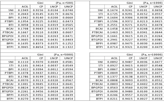
7.4 Properties of Confidence Intervals for Gini when Samples come from Pa . . . 110
7.5 Properties of Confidence Intervals for Gini when Samples come from Bu1 . . . 110
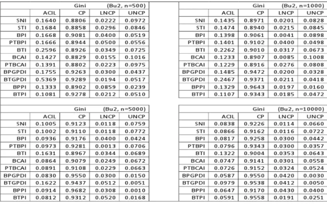
7.6 Properties of Confidence Intervals for Gini when Samples come from Bu2 . . . 111
7.7 Properties of Confidence Intervals for Gini when Samples come from Bu3 . . . 111
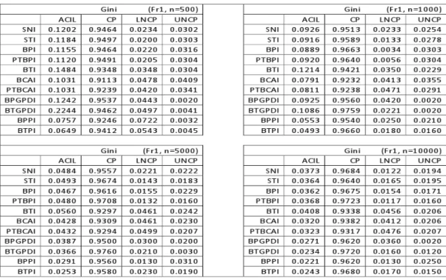
7.8 Properties of Confidence Intervals for Gini when Samples come from Fr1 . . . 112
7.9 Properties of Confidence Intervals for Gini when Samples come from Fr2 . . . 112
7.10 Properties of Confidence Intervals for Gini when Samples come from T2 . . . 113
7.11 Standard Errors for the CPs for Gini Index . . . 119
7.12 Standard Errors for the ACILs for Gini Index . . . 120
8.1 Descriptive Statistics for the Data Sets . . . 125
8.2 EVI and Nonparametric Estimates of Inequality Measures . . . 125
8.3 Nonparametric and Semi-Parametric Estimates of Inequality Measures . . . 126
8.4 Application ACILs and CPs for Gini . . . 128
8.7 Application ACILs and CPs for GE1.3 . . . 131 8.8 Application ACILs and CPs for A1 . . . 132 8.9 Application ACILs and CPs for A1.5 . . . 133 8.10 Application ACILs and CPs for A2 . . . 134 8.11 Application ACILs and CPs for QSR . . . 135 8.12 Representativeness Index for the GPD, the strict Pareto and the PPD . . . 137 D.1 Mean Squared Errors for GE0 Measure . . . 185 D.2 Mean Squared Errors for GE1 Measure . . . 186 D.3 Mean Squared Errors for GE1.3 Measure . . . 187 D.4 Mean Squared Errors for A1 Measure . . . 188 D.5 Mean Squared Errors for A1.5 Measure . . . 189 D.6 Mean Squared Errors for A2 Measure . . . 190 D.7 Mean Squared Errors for QSR Measure . . . 191 E.1 Relative Impact of Contamination on GE0 Measure . . . 193 E.2 Relative Impact of Contamination on GE1 Measure . . . 194 E.3 Relative Impact of Contamination on GE1.3 Measure . . . 195 E.4 Relative Impact of Contamination on A1 Measure . . . 196 E.5 Relative Impact of Contamination on A1.5 Measure . . . 197 E.6 Relative Impact of Contamination on A2 Measure . . . 198 E.7 Relative Impact of Contamination on QSR Measure . . . 199 F.1 Properties of Confidence Intervals for GE0 when Samples come from Pa . . . 201 F.2 Properties of Confidence Intervals for GE0 when Samples come from Bu1 . . . 201 F.3 Properties of Confidence Intervals for GE0 when Samples come from Bu2 . . . 202 F.4 Properties of Confidence Intervals for GE0 when Samples come from Bu3 . . . 202
F.5 Properties of Confidence Intervals for GE0 when Samples come from Fr1 . . . 203 F.6 Properties of Confidence Intervals for GE0 when Samples come from Fr2 . . . 203 F.7 Properties of Confidence Intervals for GE0 when Samples come from T2 . . . 204 F.8 Properties of Confidence Intervals for GE1 when Samples come from Pa . . . 205 F.9 Properties of Confidence Intervals for GE1 when Samples come from Bu1 . . . 205 F.10 Properties of Confidence Intervals for GE1 when Samples come from Bu2 . . . 206 F.11 Properties of Confidence Intervals for GE1 when Samples come from Bu3 . . . 206 F.12 Properties of Confidence Intervals for GE1 when Samples come from Fr1 . . . 207 F.13 Properties of Confidence Intervals for GE1 when Samples come from Fr2 . . . 207 F.14 Properties of Confidence Intervals for GE1 when Samples come from T2 . . . 208 F.15 Properties of Confidence Intervals for GE1.3 when Samples come from Pa . . . 209 F.16 Properties of Confidence Intervals for GE1.3 when Samples come from Bu1 . . . 209 F.17 Properties of Confidence Intervals for GE1.3 when Samples come from Bu2 . . . 210 F.18 Properties of Confidence Intervals for GE1.3 when Samples come from Bu3 . . . 210 F.19 Properties of Confidence Intervals for GE1.3 when Samples come from Fr1 . . . 211 F.20 Properties of Confidence Intervals for GE1.3 when Samples come from Fr2 . . . 211 F.21 Properties of Confidence Intervals for GE1.3 when Samples come from T2 . . . 212 F.22 Properties of Confidence Intervals for A1 when Samples come from Pa . . . 213 F.23 Properties of Confidence Intervals for A1 when Samples come from Bu1 . . . 213 F.24 Properties of Confidence Intervals for A1 when Samples come from Bu2 . . . 214 F.25 Properties of Confidence Intervals for A1 when Samples come from Bu3 . . . 214 F.26 Properties of Confidence Intervals for A1 when Samples come from Fr1 . . . 215 F.27 Properties of Confidence Intervals for A1 when Samples come from Fr2 . . . 215 F.28 Properties of Confidence Intervals for A1 when Samples come from T2 . . . 216 F.29 Properties of Confidence Intervals for A1.5 when Samples come from Pa . . . 217
F.30 Properties of Confidence Intervals for A1.5 when Samples come from Bu1 . . . 217 F.31 Properties of Confidence Intervals for A1.5 when Samples come from Bu2 . . . 218 F.32 Properties of Confidence Intervals for A1.5 when Samples come from Bu3 . . . 218 F.33 Properties of Confidence Intervals for A1.5 when Samples come from Fr1 . . . 219 F.34 Properties of Confidence Intervals for A1.5 when Samples come from Fr2 . . . 219 F.35 Properties of Confidence Intervals for A1.5 when Samples come from T2 . . . 220 F.36 Properties of Confidence Intervals for A2 when Samples come from Pa . . . 221 F.37 Properties of Confidence Intervals for A2 when Samples come from Bu1 . . . 221 F.38 Properties of Confidence Intervals for A2 when Samples come from Bu2 . . . 222 F.39 Properties of Confidence Intervals for A2 when Samples come from Bu3 . . . 222 F.40 Properties of Confidence Intervals for A2 when Samples come from Fr1 . . . 223 F.41 Properties of Confidence Intervals for A2 when Samples come from Fr2 . . . 223 F.42 Properties of Confidence Intervals for QSR when Samples come from Pa . . . 224 F.43 Properties of Confidence Intervals for QSR when Samples come from Bu1 . . . 224 F.44 Properties of Confidence Intervals for QSR when Samples come from Bu2 . . . 225 F.45 Properties of Confidence Intervals for QSR when Samples come from Bu3 . . . 225 F.46 Properties of Confidence Intervals for QSR when Samples come from Fr1 . . . 226 F.47 Properties of Confidence Intervals for QSR when Samples come from Fr2 . . . 226 G.1 Standard Errors for the CPs for GE0 . . . 228 G.2 Standard Errors for the ACILs for GE0 . . . 229 G.3 Standard Errors for the CPs for GE1 . . . 230 G.4 Standard Errors for the ACILs for GE1 . . . 231 G.5 Standard Errors for the CPs for GE1.3 . . . 232 G.6 Standard Errors for the ACILs for GE1.3 . . . 233 G.7 Standard Errors for the CPs for A1 . . . 234
G.8 Standard Errors for the ACILs for A1 . . . 235 G.9 Standard Errors for the CPs for A1.5 . . . 236 G.10 Standard Errors for the ACILs for A1.5 . . . 237 G.11 Standard Errors for the CPs for A2 . . . 238 G.12 Standard Errors for the ACILs for A2 . . . 239 G.13 Standard Errors for the CPs for QSR . . . 240 G.14 Standard Errors for the ACILs for QSR . . . 241
Chapter
1
Introduction
Statistical inference is the process of drawing conclusions from data that are subject to random varia-tion. More substantially, the terms statistical inference, statistical induction and inferential statistics are used to describe systems of procedures that can be used to draw conclusions from data sets arising from systems affected by random variation. See e.g. the 2008 Oxford Dictionary of Statistics. Initial requirements of such a system of procedures for inference and induction are that the system should produce reasonable answers when applied to well-defined situations and that it should be general enough to be applied across a range of situations. There are many contexts in which inference is desirable, and there are many approaches to performing inference. This study particularly addresses statistical inference for inequality measures based on semi-parametric estimators. In this chapter we briefly give some background ideas and we state the problem under consideration. We then describe the scope of the study and we give its main contributions. Finally we provide an outline of the chapters to follow.
1.1
Background and Problem Statement
Economic inequality is an important concept in any society and even more so in a developing country where often a high level of inequality exists. It is therefore essential that reliable measures of inequality be defined and their properties investigated. Such measures, also used as measures of concentration or diversity, are very popular in economics and especially in measuring the inequality in income or wealth within a population and between populations. However, they have applications in many other fields such as ecology (see e.g. Magurran [40]), linguistics (see e.g. Herdan [31]), sociology (see e.g. Allison [1]), demography (see e.g. White [55]), epidemiology (see e.g. Harper and Lynch [30]) and
information science (see e.g. Rousseau [48]), just to mention a few.
Over the years a large number of these measures have been proposed. Some of the most well known ones are the Gini index, the generalized entropy, the Atkinson and the quintile share ratio measures. Recently the Laeken European Council has adopted the so called Laeken Indicators which cover four important dimensions of social inclusion (financial poverty, employment, health and education), highlighting the multidimensionality of the phenomenon of social exclusion. Some of these indicators are measures of inequality. In particular, they include the Gini index and the quintile share ratio. Having reliable inequality measures available is an important first step. A next step is to estimate the values of these measures using samples from the appropriate populations and, in particular, to estimate the variability of these estimators and more generally, to obtain confidence intervals for these measures. Since inequality is inherently dependent on the tails of a population, estimators of inequality are typically overly sensitive to data from these tails. We note in this regard that all the well known inequality measures have unbounded influence functions. It is well known that income distributions often exhibit a long tail to the right, making estimators of inequality particularly sensitive to large values. It is thus important to study the behavior of estimators based on data from heavy-tailed distributions. Many of the traditional estimators are sensitive to such extreme data points (see e.g. Cowell and Flachaire [10]) and remedial action needs to be taken. This remedial action can be either a trimming of the extreme data or a modification of the estimator to make it more robust to extreme observations. Cowell and Flachaire [10] (see also Cowell and Victoria-Feser [12]) have proposed a so-called semi-parametric approach to modify estimators under heavy-tailed distributions. This method estimates the left part of the distribution, where the bulk of the distribution resides, using the usual nonparametric em-pirical distribution function and the right (upper) part of the distribution using a Pareto distribution. The resulting estimator is therefore partly nonparametric and partly parametric, hence semi-parametric. Based on their idea, results from extreme value theory are used in this thesis to obtain more reli-able distribution estimators. These new estimators of the distribution form the basis for more robust estimators of the measures of inequality.
The bootstrap has in recent years become a very powerful technique for estimating variances of com-plex statistics and obtaining confidence intervals based on such statistics (see e.g. Efron and Tibshi-rani [26]). It has also been applied successfully to estimators of some inequality measures (see e.g. Davidson and Flachaire [18]). This is an extremely useful technique that can also be applied in the semi-parametric setting.
1.2
Scope and Contributions of the Study
Given a data set, a very important issue is to determine from which distribution the data are likely to have come from. In practice many methods are based on the empirical distribution function, which can lead to misleading conclusions especially when dealing with heavy-tailed distributions, e.g. income distributions. The main objective of this thesis is to develop improved inference for inequality measures in the case of heavy-tailed distributions. We use tools from Extreme Value Theory as basis from which to propose estimators for measures of inequality in a semi-parametric setting. The main contributions of this thesis are as follows.
1. We develop new semi-parametric estimators for the underlying distribution based on results from Extreme Value Theory (EVT). This is done by fitting three different parametric distributions in the tails, namely the Generalized Pareto distribution (GPD), the strict Pareto distribution, and the Perturbed Pareto Distribution (PPD).
2. Over the years nonparametric estimators for inequality measures have been used. Using the semi-parametric estimators for the underlying distribution, we develop semi-parametric estima-tors for four important measures of inequality, namely the Gini index, the Generalized Entropy (GE), the Atkinson and the Quintile Share Ratio (QSR) measures.
3. The influence function of the QSR and the limiting distribution of its nonparametric estimator are not available in literature. Both of these are derived in this study.
4. Sampling distributions of the semi-parametric estimators are studied via simulation. It is shown that the sampling distributions of semi-parametric estimators are better approximated by the limiting normal distribution.
5. With an extensive simulation study we show that in terms of mean squared errors, the semi-parametric estimators show improved performance over the nonsemi-parametric estimators as well as over the proposal of Cowell and Flachaire [10].
6. With an extensive simulation, we study the sensitivity of the estimators to outliers. Using the relative impact of contamination, we show that the proposed semi-parametric estimators are less sensitive to contamination or outliers than their nonparametric counterparts.
7. We carry out an extensive simulation to study confidence intervals for the inequality measures. Various confidence intervals were considered, viz. the standard normal, the Studentt and
boot-strap intervals. These confidence intervals were obtained based on both the traditional estima-tors as well as on the semi-parametric estimaestima-tors. In the simulation we studied the performance of the intervals in terms of the average confidence interval lengths and coverage probabilities. It appeared in most cases that confidence intervals based on semi-parametric estimators outper-form the methods based on traditional estimators. Given the fact that confidence intervals are obtained for complex measures, the proposed procedures do remarkably well. The performance of the bootstrap is also remarkably good, given the complexity of the statistics underlying the bootstrap procedures.
8. Illustrations are given in order to show how the methods developed can be applied to real life data sets. The usual methods as well as the semi-parametric ones are applied to three data sets, claims data from a South African short term insurer, Norwegian fire insurance data and 2005 South African income and expenditure survey data. The illustrations show that the proposed procedures do remarkably well and can be used in practice to reach satisfactory conclusions. In order to choose between the three parametric distributions, we propose that a measure of sample representativeness be used. This was applied to the three data sets to choose the appropriate parametric distribution to use in the tail estimation.
1.3
Outline of the Study
In Chapter 2 we provide a list of definitions of inequality measures and their properties, and we give an overview of the approaches to the inequality measurement. Chapter 3 is devoted to describing a num-ber of popular heavy-tailed distributions. In that chapter we also study the sampling distributions of the nonparametric estimators of the inequality measures described in Chapter 2. In Chapter 4 we review some methods of estimating the Extreme Value Index (EVI) and choosing the threshold above which to apply the parametric distribution when estimating the underlying distribution in a semi-parametric setting. In Chapter 5 we discuss the semi-parametric estimation of measures of inequality, in par-ticular, the Gini, the generalized entropy, the Atkinson and the quintile share ratio measures. In the same chapter we also study the sampling distributions of the semi-parametric estimators. Chapter 6 provides an overview of various methods for constructing confidence intervals. A simulation study is conducted in Chapter 7 in order to assess some properties of the estimators and their performance in terms of confidence intervals. Chapter 8 illustrates how the different techniques described can be used in practice. Chapter 9 is devoted to conclusions and to indicate some areas that can be investigated in
Chapter
2
Literature Overview
A large body of literature is devoted to the measurement of inequality. Many papers showed how to approach the measurement of inequality statistically, by describing the use of typical sample designs. However, extreme values in the data can have a detrimental effect on the estimators of inequality measures, especially when using some of the classical methods of estimation. This problem has been tackled by some authors. In this chapter we provide a list of definitions of inequality indices and their properties, and we give an overview of the approaches to inequality measurement. We start off by introducing the Lorenz curves and the influence functions.
2.1
Lorenz Curves
Lorenz curves constitute an important tool for analyzing economic inequality. As mentioned by Schluter and Trede [50], in the case of income distribution the Lorenz curve depicts the cumulative income share of the least well-off fraction of the population.
Definition 2.1. Let ℑ be the set of all univariate probability distributions with support(0,∞), and let
X be a random variable with probability distribution F ∈ℑ. The Lorenz curve of X is given by (see Schluter and Trede [51])
{(q,C(F;q)),0≤q≤1}, (2.1) whereCis the cumulative functional defined by
C(F;q) = Z ∞ 0 x1{x≤F−1(q)}dF(x) = Z F−1(q) 0 xdF(x), (2.2)
Consider the normalized functional
L(F;q):=C(F;q)
µ , (2.3)
whereµ=C(F; 1)is the mean functional.
The graph ofC(F;q)versusqdescribes the generalized Lorenz curve (GLC), and the graph ofL(F;q) versusqdescribes the relative Lorenz curve (RLC).
A Lorenz curve shows the degree of inequality that exists in the distributions, and is often used to illustrate the extent to which income or wealth is distributed unequally in a particular society. As we will later see, many inequality measures are closely related to the Lorenz curve.
2.2
Influence Functions
In robust statistics the influence function was developed as an important measure of sensitivity of estimators to large values. See e.g. Huber and Ronchetti [33] for discussion of this.
Definition 2.2. Let∆z be a point mass distribution giving probability1to an arbitrary pointz∈(0,∞).
Define the mixture distribution
Fε(z)(x) = (1−ε)F(x) +ε∆z(x), forε∈[0,1]. (2.4)
The influence function (IF) of a functionalT(F)is defined as
IF(z;T) =lim ε→0 T(Fε(z))−T(F) ε = ∂ ∂εT(F (z) ε )|ε=0. (2.5) Remark 2.1.
1. The relative influence function (RIF) is defined as
RIF(T) =IF(z;T)
T(F) . (2.6)
2. The functionalT(F)can be estimated by the plug-in estimatorT(Fn), whereFnis the empirical distribution function of the sampleX1,X2, . . . ,Xn, defined by
Fn(x) =1 n n
∑
i=1 1{Xi≤x}. (2.7)The relative impact of a contamination on the functionalT is defined by RIC(T) = T(Fn)−T(F ? n) T(Fn) , (2.8)
whereFn?is the empirical distribution function of the contaminated sample. See e.g. Cowell and Flachaire [10].
2.3
Inequality Measures: Definitions and Some Properties
In order to measure inequality, a number of coefficients such as the generalized entropy (GE), the Atkinson, the quintile share ratio and the Gini measures, have been introduced in the literature. In this section we describe these inequality measures and we give some of their properties.
2.3.1
Generalized Entropy Measures of Inequality
The concept of comparing distributions using information-theoretic approaches has involved using entropy-based measures which quantify the discrepancies between the probability distributions (see Cowell et al. [11]). First introduced by Shannon [53], this concept was further developed into a rela-tive measure of entropy by Kullback and Leibler [38]. Cowell et al. [11] then showed that generalized entropy measures are obtained by a change of variables from these entropy measures.
LetY be a random variable distributed on the nonnegative real line, and let f be its probability density function. The generalized entropy (GE) inequality measure is defined by (see e.g. Cowell and Flachaire [10], Cowell et al. [11]): IEα = Z ∞ 0 1 α(α−1) y µ1 α −1 dF(y) = 1 α(α−1) µ α µα 1 −1 , α6=0,1, (2.9) where µα= Z ∞ 0 yαdF(y)andµ1=E(Y).
The motivation of Equation (2.9) is as follows: Consider Shannon’s entropy defined as the expected information (see Shannon [53])
H(f):=−E[logf(Y)] =−
Z ∞
0
Letting g(f) =−logf, we see that g is convex withg(1) =0. It also has an additive property. The latter property is not essential and the above can be generalized to functionsgα which are convex and for whichgα(1) =0(see e.g. Khinchin [35]).
An important special case is given by
gα(f) = 1
α−1[1−f
α],
α>0,α6=1. (2.11) From (2.11), a generalization of (2.10) is obtained as
Hα(f):=Egα(f(Y)) = 1 α−1 1−E f(Y)α−1 , α>0,α6=1. (2.12) In order to link this entropy to inequality, the transformations:[0,1]→[0,1]given below can be used (see Cowell et al. [11]).
Define s(q):= F −1(q) R1 0 F−1(t)dt = y µ1 , (2.13)
whereF is the distribution function ofY such that a proportionq=F(y)of the population has a value less thany,µ1is the mean of the distribution. See [11] for an interpretation of the transformations. It is clear that the functionshas the same properties as a regular density function:
s(q)≥0, for allqand
Z 1
0
s(q)dq=1. (2.14)
Substitutingsfor f in Equation (2.12) leads to
Hα(s) =−αIEα. (2.15)
Thus
Iα
E =−α−1Hα(s). (2.16)
As mentioned in [11], the parameter αhas a natural interpretation in terms of economic welfare: for α>0, the measureIEα is “top-sensitive” in that it gives higher importance to changes in the top of the distribution.
The equivalent measure for a finite populationy1,y2, . . . ,yN, is given in Cowell [9] as Iα E = 1 α(α−1) " 1 N N
∑
i=1 yi y α −1 # , (2.17) where y= 1 N N∑
i=1 yi.The influence function ofIα
E is given by IF(z;Iα
E) = [zα−µα]−
µα
(α−1)µα1+1[z−µ1],α6=0,1, (2.18)
see Cowell and Flachaire [10], and for any given value ofα, it is unbounded: 1. Ifα>1the IF tends to infinity whenz→∞at the rate ofzα;
2. If0<α<1the IF tends to infinity whenz→∞at the rate ofz;
3. Ifα<0the IF tends to infinity whenz→∞at the rate ofz, and whenz→0at the rate ofzα.
Mean Logarithmic Deviation
The mean logarithmic deviation (MLD) measure is a special case of the GE class where α=0. It follows directly from Equation (2.16) that
IE0 =− Z ∞ 0 log y µ1 dF(y) =logµ1−ν, (2.19) where ν= Z ∞ 0 (logy)dF(y).
The influence function, given by
IF(z;IE0) =−[logz−ν] + 1
µ1[z−µ1], (2.20)
tends to infinity at the ratezwhenz→∞and at the rate oflogzwhenz→0.
Insti-tute [56]) IE0= 1 N N
∑
i=1 log y yi . (2.21) Theil MeasureThe Theil measure of inequality is also a special case of the GE class whereα=1. It follows directly from Equation (2.16) that it is given by:
IE1= Z ∞ 0 y µ1 log y µ1 dF(y) = ν µ1 −logµ1, (2.22) where now ν= Z ∞ 0 ylogydF(y).
The influence function, given by
IF(z;IE1) = 1
µ1
[zlogz−ν]−ν+µ1
µ21 [z−µ1], (2.23)
tends to infinity at the rate ofzlogzwhenz→∞.
The Theil Coefficient for a finite populationy1,y2, . . . ,yN, is given by (see [56]):
IE1= 1 N N
∑
i=1 yi y log yi y . (2.24)2.3.2
Atkinson Class of Inequality Measures
The Atkinson measure of inequality is defined by (see Cowell and Flachaire [10]):
IAε =1− " Z ∞ 0 y µ 1−ε dF(y) #1/(1−ε) =1−µ 1/(1−ε) 1−ε µ , ε>0,ε6=1, (2.25) where µ1−ε= Z ∞ 0 y1−εdF(y).
The special case whereε=1is given by
IA1=1−e
R∞
0(logy)dy
µ =1−e
The Atkinson measureIε
Ais a nonlinear transformation of the GE measureIEα: forε=1−α>0, I1−α
A =1−[(α
2−α)Iα
E+1]1/α.
With that relationship the Atkinson measures basically play the same role as the generalized entropy measures. See Cowell et al. [11].
The influence function, given by (see Cowell and Flachaire [10])
IF(z;Iε A) = µ11/−(1−ε) ε (ε−1)µ[z 1−ε−µ 1−ε] + µ11/−(1−ε) ε µ2 [z−µ], (2.27)
has the following properties:
1. If0<ε<1the IF tends to infinity whenz→∞at the rate ofz;
2. Ifε>1the IF tends to infinity whenz→∞at the rate ofz, and whenz→0at the rate ofz1−ε.
Forε=1, the influence function is given by
IF(z;IA1) =−e R∞ 0 (logy)dy µ [logz− Z ∞ 0 (logy)dy] +e R∞ 0(logy)dy µ2 [z−µ], (2.28)
which tends to infinity whenz→∞at the rate ofz, and whenz→0at the rate oflogz. The Atkinson measure of inequality for a finite populationy1,y2, . . . ,yN, is given by (see [56]):
Iε A=1− " 1 N N
∑
i=1 yi y 1−ε#1/(1−ε) , ε6=1, (2.29) and IA1=1−1 y N∏
i=1 (y1i/N). (2.30)2.3.3
Relationship Between the Lorenz Curve and the GE Measures and
Between the Lorenz Curve and Atkinson Measures
The relative Lorenz curve was defined in Equation (2.3) as
Consider the quantile function Q(F;q)≡F−1(q) =inf{x|F(x)≥q}. (2.32) Note that L0(F;q)≡ d dqL(F;q) =µ −1Q(F;q). (2.33) Since Iα E = [α(α−1)]−1 Z ∞ 0 y µ α −1 dF(y), (2.34) it follows that Iα E = [α(α−1)]−1 Z 1 0 h µ−1Q(F;u)α−1idu= [α(α−1)]−1 Z 1 0 h L0(F;u)α−1idu. (2.35) Similarly, we have IAε=1− Z 1 0 µ−1Q(F;u)1−εdu 1/(1−ε) =1− Z 1 0 L0(F;u)1−εdu 1/(1−ε) . (2.36)
2.3.4
Gini Coefficient
The Gini Coefficient is the most widely used measure of inequality. It is defined by (see e.g. Cowell and Flachaire [10]):
IG=1−2
Z 1
0
L(F;p)d p, (2.37)
whereL(.)denotes the Lorenz curve as given in Equation (2.3).
The Gini coefficient lies between0and1. The value 0corresponds to perfect equality and the value 1 corresponds to perfect inequality. In an economic situation, perfect equality means the wealth is uniformly distributed over all the individuals in the population, and perfect inequality means the entire wealth goes to only one individual.
Letting A= Z 1 0 L(F;p)d p and B= Z 1 0 pd p= 1 2,
it easily follows from Equation (2.37) that
IG=2(B−A),
therefore, twice the area between the45°line and the Lorenz curve, lying below the line.
From Pan American Health Organization [43], the Lorenz curve is an accumulated frequency curve that compares the distribution of a specific variable with the uniform distribution that represents equality. This equality distribution is represented by a straight line of slope one, and the greater the deviation of the Lorenz curve from this line, the greater the Gini Coefficient.
Many alternative expressions for Gini have been given in the literature. The most important ones are the following (see e.g. Davidson [17], Dorfman [21], Duclos and Araar [24]):
• IG= 2 µ Z ∞ 0 yF(y)dF(y)−1, (2.38) • IG=1−2 µ Z ∞ 0 y(1−F(y))dF(y), (2.39) • IG=1 µ Z ∞ 0 (2F(y)−1)ydF(y), (2.40) • IG=1−1 µ Z ∞ 0 (1−F(y))2dy, (2.41) • IG= 1 µ Z ∞ 0 F(y)(1−F(y))dy, and (2.42) • IG= E|X−Y| 2µ , (2.43)
whereX andY are independent, having the same distribution functionF with meanµ.
Remark 2.2. These formulas for the Gini coefficient are all related to one another. These relationships will now be proved.
• Equation (2.39) is derived from Equation (2.38) as follows: IG= 2 µ Z ∞ 0 yF(y)dF(y)−1 = 2 µ − Z ∞ 0 y(1−F(y))dF(y) +µ −1 =−2 µ Z ∞ 0 y(1−F(y))dF(y) +2−1 =1−2 µ Z ∞ 0 y(1−F(y))dF(y).
• Equation (2.40) is derived from Equation (2.38) as follows:
IG=2 µ Z ∞ 0 yF(y)dF(y)−1 =1 µ Z ∞ 0 2yF(y)dF(y)−µ =1 µ Z ∞ 0 2yF(y)dF(y)− Z ∞ 0 ydF(y) =1 µ Z ∞ 0 (2F(y)−1)ydF(y).
• Equation (2.39) is derived from Equation (2.37) as follows:
IG=1−2 Z 1 0 L(F;p)d p =1−2 µ Z 1 0 Z F−1(p) 0 ydF(y)d p =1−2 µ Z ∞ 0 y Z 1 F(y) d pdF(y) =1−2 µ Z ∞ 0 y(1−F(y))dF(y).
• Equation (2.41) is derived from Equation (2.39) as follows:
IG=1−2 µ Z ∞ 0 y(1−F(y))dF(y) =1+2 µ Z ∞ 0 y(1−F(y))d(1−F(y)) =1−2 µ Z ∞ 0 (1−F(y))2dy+2 µ Z ∞ 0 y(1−F(y))dF(y)
(by integration by parts) =1−2
µ
Z ∞
0
It follows that 2IG=2−2 µ Z ∞ 0 (1−F(y))2dy, thus IG=1−1 µ Z ∞ 0 (1−F(y))2dy.
• Equation (2.42) is derived from Equation (2.41) as follows:
IG=1−1 µ Z ∞ 0 (1−F(y))2dy =1−1 µ Z ∞ 0 (1−F(y))(1−F(y))dy =1−1 µ Z ∞ 0 (1−F(y))dy+1 µ Z ∞ 0 F(y)(1−F(y))dy = 1 µ Z ∞ 0 F(y)(1−F(y))dy.
• Equation (2.43) is derived from Equation (2.39) as follows:
E|X−Y|= Z ∞ 0 Z ∞ 0 |x−y|dF(x)dF(y) =2 Z ∞ 0 Z x 0 (x−y)dF(y)dF(x) =2 Z ∞ 0 xF(x)dF(x)−2 Z ∞ 0 Z x 0 ydF(y)dF(x) =−2 Z ∞ 0 x(1−F(x))dF(x) +2µ−2 Z ∞ 0 y(1−F(y))dF(y) =2µ−4 Z ∞ 0 y(1−F(y))dF(y) =2µ 1−2 µ Z ∞ 0 y(1−F(y))dF(y)
=2µIG(using Equation (2.39)),
thus
IG=
E|X−Y|
2µ .
In our subsequent work, use will be made of Equation (2.42) for the Gini coefficient, as it is very convenient for estimation purposes.
The influence function ofIGis given by (see e.g. Cowell and Flachaire [10]) IF(z;I ) =2
R(F)−C(F;F(z)) + z(R(F)−(1−F(z)))
where
R(F) =
Z 1
0
L(F;p)d p (2.45)
andCis as given in Equation (2.2).
This influence function tends to infinity at the rate ofzwhenz→∞.
Remark 2.3. The above formulation of the Gini coefficient has been given for the case of an infinite population. In the case of finite populations, the integrals must be replaced by the corresponding sums. For example in this case Equation (2.43) becomes
IG= 1 2N2y N
∑
i=1 N∑
j=1 |yj−yi| (2.46)for a finite populationy1,y2, . . . ,yN.
2.3.5
Quintile Share Ratio Measure of Inequality
Consider a random variableY with distribution functionF and denote byQ its quantile function. For simplification purposes we will useQ(q)forQ(F;q)defined in Equation (2.32).
Definition 2.3. The quintile share ratio (QSR) is defined by
η= R∞ Q(0.8)ydF(y) RQ(0.2) 0 ydF(y) = EY1{Y >Q(0.8)} EY1{Y ≤Q(0.2)}, (2.47)
where1{.}is an indicator function.
In the case of income, the QSR can be interpreted as the ratio of the total income received by the20% of a country’s population with highest income to that received by the20%of the country’s population with the lowest income (see Hulliger and Schoch [34]).
The QSR for a finite populationy1,y2, . . . ,yN, is given by:
η= " N
∑
i=[0.8N]+1 Yi,N # / "[0.2N]∑
i=1 Yi,N # , (2.48)whereY1,N<Y2,N < . . . <YN,N are the order statistics associated with the finite population and[x]is the largest integer smaller than or equal tox.
Remark 2.4. The QSR forms part of the so-called Laeken indicators, the European indicators on poverty and social exclusion (see EU-SILC [28]).
The influence function of the QSR is not available yet in the literature. This is derived in the next theorem.
Theorem 2.1. The influence function of the quintile share ratioηin Equation (2.47) is given by:
IF(z;η) = [−zN(F) +0.2Q(0.8)D(F) +0.8Q(0.2)N(F)]/D2(F), ifz≤Q(0.2), [0.2Q(0.8)D(F)−0.2Q(0.2)N(F)]/D2(F), ifQ(0.2)<z≤Q(0.8), [zD(F)−0.8Q(0.8)D(F)−0.2Q(0.2)N(F)]/D2(F), ifz>Q(0.8), (2.49) where N(F) = Z ∞ Q(0.8) xdF(x) (2.50) and D(F) = Z Q(0.2) 0 xdF(x). (2.51)
Proof. Consider the mixture distributionFε,zdefined in Equation (2.4), and define the influence function
as in Equation (2.5). Denoting byQ(εz)the quantile function associated withFε(z), we have lim ε→0 1 ε Z ∞ Q(εz)(0.8) xdF(x)− Z ∞ Q(0.8) xdF(x) = ∂ ∂ε Z ∞ Q(εz)(0.8) xdF(x)|ε=0 =−Q(εz)(0.8)f(Q(εz)(0.8)) ∂ ∂εQ (z) ε (0.8)|ε=0 =−Q(0.8)f(Q(0.8))IF(z;Q(0.8)).
It follows that forε→0,
Z ∞ Q(εz)(0.8) xdF(x) = Z ∞ Q(0.8) xdF(x)−εQ(0.8)f(Q(0.8))IF(z;Q(0.8)) +o(ε) =N(F)−εQ(0.8)f(Q(0.8))IF(z;Q(0.8)) +o(ε).
On the other hand we have
ε Z ∞ Q(εz)(0.8) xd∆z(x) =εz1(z≥Q (z) ε (0.8)) =εz1(z≥Q(0.8))(1+o(1)).
Therefore N(Fε(z)) = (1−ε) Z ∞ Q(εz)(0.8) xdF(x) +ε Z ∞ Q(εz)(0.8) xd∆z(x) = (1−ε) [N(F)−εQ(0.8)f(Q(0.8))IF(z;Q(0.8)) +o(ε)] +ε Z ∞ Q(εz)(0.8) xd∆z(x) =N(F)−εN(F)−εQ(0.8)f(Q(0.8))IF(z;Q(0.8)) +εz1(z≥Q(0.8)) +o(ε). It follows that lim ε→0 N(Fε(z))−N(F) ε =−N(F)−Q(0.8)f(Q(0.8))IF(z;Q(0.8)) +z1(z≥Q(0.8)) ≡N0(F). (2.52) Similarly we have lim ε→0 1 ε " Z Q(εz)(0.2) 0 xdF(x)− Z Q(0.2) 0 xdF(x) # = ∂ ∂ε Z Q(εz)(0.2) 0 xdF(x)|ε=0 =Q(εz)(0.2)f(Q(εz)(0.2)) ∂ ∂εQ (z) ε (0.2)|ε=0 =Q(0.2)f(Q(0.2))IF(z;Q(0.2)), leading to Z Q(εz)(0.2) 0 xdF(x) = Z Q(0.2) 0 xdF(x) +εQ(0.2)f(Q(0.2))IF(z;Q(0.2)) +o(ε) =D(F) +εQ(0.2)f(Q(0.2))IF(z;Q(0.2)) +o(ε). Furthermore we have, ε Z Q(z) ε (0.2) 0 xd∆z(x) =εz1(z≤Q (z) ε (0.2)) =εz1(z≤Q(0.2))(1+o(1)).
It follows that D(Fε(z)) = (1−ε) Z Q(εz)(0.2) 0 xdF(x) +ε Z Q(εz)(0.2) 0 xd∆z(x) = (1−ε) [D(F) +εQ(0.2)f(Q(0.2))IF(z;Q(0.2)) +o(ε)] +ε Z Q(εz)(0.2) 0 xd∆z(x) =D(F)−εD(F) +εQ(0.2)f(Q(0.2))IF(z;Q(0.2)) +εz1(z≤Q(0.2)) +o(ε). Therefore, lim ε→0 D(Fε(z))−D(F) ε =−D(F) +Q(0.2)f(Q(0.2))IF(z;Q(0.2)) +z1(z≤Q(0.2)) ≡D0(F). (2.53)
The influence function for the QSRηis then given by lim ε→0 ηε−η ε = ∂ ∂εηε|ε=0 = ∂ ∂ε N(Fε(z)) D(Fε(z)) |ε=0 = N 0(F)D(F)−D0(F)N(F) D2(F) . (2.54) But N0(F)D(F)−D0(F)N(F) =D(F) [−N(F)−Q(0.8)f(Q(0.8))IF(z;Q(0.8)) +z1(z≥Q(0.8))] −N(F) [−D(F) +Q(0.2)f(Q(0.2))IF(z;Q(0.2)) +z1(z≤Q(0.2))] =−D(F)Q(0.8)f(Q(0.8))IF(z;Q(0.8)) +zD(F)1(z≥Q(0.8)) −N(F)Q(0.2)f(Q(0.2))IF(z;Q(0.2))−zN(F)1(z≤Q(0.2)) and IF(z;Q(p)) = ∂ ∂εQ (z) ε (p)|ε=0 = ∂ ∂εF −1 ε (p)|ε=0, where
as in Equation (2.4).
In order to find the above derivative, we use the relationship
Fε(Fε−1(p)) =p.
Differentiating this expression on both sides, using the rules of differentiating a composite function, gives ∂ ∂εFε(F −1 ε (p)) =0⇒ ∂ ∂xFε(x)|x=Fε−1(p)· ∂ ∂εF −1 ε (p) + ∂ ∂εFε(x)|x=Fε−1(p)=0 ⇒ ∂ ∂ε Fε−1(p) =−∂ ∂ε Fε(x)|x=F−1 ε (p)· ∂ ∂x Fε(x)|x=F−1 ε (p) −1 ⇒ ∂ ∂εF −1 ε (p) =− ∂ ∂εFε(x)|x=Fε−1(p)· fε(Fε−1(p))−1.
Finally, taking the limit asε→0gives ∂ ∂εF −1 ε (p)|ε=0= [p−1(z<Q(p))]f(Q(p)) −1. (2.55) Thus IF(z;Q(p)) = 1 f(Q(p)(p−1(z<Q(p))). (2.56) Substituting the terms into Equation (2.54) gives directly
IF(z;η) = [−zN(F) +0.2Q(0.8)D(F) +0.8Q(0.2)N(F)]/D2(F), ifz≤Q(0.2), [0.2Q(0.8)D(F)−0.2Q(0.2)N(F)]/D2(F), ifQ(0.2)<z≤Q(0.8), [zD(F)−0.8Q(0.8)D(F)−0.2Q(0.2)N(F)]/D2(F), ifz>Q(0.8). (2.57)
This completes the proof of the theorem.
Remark 2.5.
1. The fact that
IF(z;η) = [0.2Q(0.8)D(F)−0.2Q(0.2)N(F)]/D2(F) =Constant
for QF(0.2)<z<QF(0.8)is due to the fact that the definition of the QSR does not take into
account the data values between QF(0.2) andQF(0.8); that is, those values do not influence the QSR measure.
2. Given the plug-in estimatorη(Fn)ofη(F)≡η, we will have (under appropriate conditions) that √ n(η(Fn)−η(F))→D N 0,σ2η, (2.58) where σ2η= Z ∞ 0 IF2(z;η)dF(z). (2.59) The varianceσ2η can be estimated using the plug-in method.
2.4
Current Estimation Procedures and Effects of Extreme Values
Having reliable inequality measures available is an important first step. A next step is to estimate the values of these measures using samples from the appropriate populations and, in particular, to estimate the variability of these estimators and more generally, to obtain confidence intervals for the measures. Since inequality is inherently dependent on the tails of a population, estimators of inequality are typically sensitive to data from these tails. In this section we discuss various approaches to the estimation problem.2.4.1
Income Distribution and Inequality Measurement: The Problem of
Extreme Values
Inequality measures can be very sensitive to changes in the distribution. In the case of income dis-tribution for example, the data often has a long right tail, and this can seriously affect the estimation procedures for the measures. Thus it is appropriate to examine the behavior of inequality measures with respect to extreme values (see Cowell and Flachaire [10]). In [10] they examined statistical perfor-mance of inequality indices in the presence of extreme values in data and showed that these indices are very sensitive to the properties of the income distribution. They considered various inequality mea-sures (Generalized entropy (GE), MLD Coefficient (GE withα=0), Theil Coefficient (GE withα=1), Atkinson, LogVar and Gini measures) in a semi-parametric, an asymptotic and a bootstrap setup. In the case of the bootstrap, two nonstandard methods were used: moon bootstrap (mout onnbootstrap) and semi-parametric bootstrap. In order to carry out their analysis, they made use of three different dis-tributions: the Singh-Maddala, the Pareto and the lognormal distributions. All those distributions will be discussed further in this work (see Chapter 3). Amongst others, the following points were emphasized
in [10].
1. The GE measures withα>1are very sensitive to high incomes in the data.
2. The Gini Coefficient is less sensitive to contamination in high incomes than the GE class of measures.
3. The inequality measures computed with a semi-parametric estimation of the income distribution are much less sensitive to contamination.
4. The MLD Coefficient is more sensitive to contamination in high incomes when the underlying distribution has a heavy upper tail. Semi-parametric MLD measures are much less sensitive. We will investigate the semi-parametric procedures further in this work (see e.g. Chapter 5).
2.4.2
Asymptotic and Bootstrap Inference for Inequality Measures
Bootstrap techniques are useful tools for estimating properties of estimators (e.g. variances, standard errors), by calculating them when sampling from a given data set, or from an approximating distribution. One standard choice for an approximating distribution is the empirical distribution of the observed data. The bootstrap method offers an ideal opportunity to perform approximate inference. Using Monte Carlo results, Davidson and Flachaire [18] noticed that bootstrapping a commonly used measure of inequality leads to inference which is not accurate even in very large samples, although inference with poverty measures is satisfactory. They found that the major cause is the extreme sensitivity of many inequality measures to the exact nature of the upper tail of the income distribution. As a solution, they proposed two nonstandard bootstrap methods: the mout of nbootstrap, which is valid in some situations where the standard bootstrap fails, and a semi-parametric bootstrap in which the upper tail is modeled parametrically.
Through their experiment, they found three reasons for the poor performance of standard bootstrap techniques:
1. Almost all indices are nonlinear functions of sample moments, thereby inducing biases and nonnormality in estimators of these indices.
2. Estimators of the covariances of the sample moments used to construct indices are often very noisy.
3. The indices are often extremely sensitive to the exact nature of the tails of the distribution. The simulation results showed that the third cause is often the most important. In order to circumvent this problem, the following two bootstrap techniques were proposed (see [18]):
1. The m out of n bootstrap: It is valid in the case of infinite variance. It consists of drawing subsamples of sizemfrom the original sample of sizen(withn≥m), without replacement. This technique is also known as the moon bootstrap and is usually thought of as useful when the standard bootstrap fails or when it is difficult to check its consistency.
2. The semi-parametric bootstrap: It consists of drawing samples from a semi-parametric esti-mator of the distribution, which combines a parametric estimation of the upper tail with a non-parametric estimation of the rest of the distribution.
Davidson and Flachaire [18] analyzed the Theil inequality measure and showed that asymptotic and standard bootstrap tests for it may not yield accurate inference, even if the sample size is very large. The main reason for this, they said, is the nature of the upper tail of the income distribution. Their proposed methods performed better than standard bootstrap techniques.
2.4.3
Further Developments on Measures of Inequality
Eliazar and Sokolov [27] established a Gini-based characterization of extreme value statistics, presen-ting a novel connection between the Gini index and extreme value statistics.
Qin et al. [45] constructed empirical likelihood confidence intervals for the Gini coefficient and showed that these perform very well for large samples. However, the method has under-coverage problems when the sample size is small or moderate. To solve that problem they proposed the bootstrap-calibrated empirical likelihood confidence intervals.
Langel and Tillé [39] proposed an improved methodology for the estimation of the QSR and the variance of the estimator in a complex sampling design framework. They also discussed the cons-truction of confidence intervals and made a proposition to account for skewness of the sampling dis-tribution of the QSR. Realizing that the skewness in the disdis-tribution of the estimators of the quintile share ratio makes it difficult to achieve reliable confidence intervals, the authors applied the Box-Cox transformations to reduce the problems caused by skewness. They applied their method to a real life data set and pointed out the common problem of skewness, and the sensitivity of statistics to extreme
C