This is a repository copy of Quantum-based subgraph convolutional neural networks.
White Rose Research Online URL for this paper:
http://eprints.whiterose.ac.uk/139142/
Version: Accepted Version
Article:
Zhang, Zhihong, Chen, Dongdong, Wang, Jianjia et al. (2 more authors) (2018)
Quantum-based subgraph convolutional neural networks. Pattern recognition. 38 - 49.
ISSN 0031-3203
https://doi.org/10.1016/j.patcog.2018.11.002
Reuse
This article is distributed under the terms of the Creative Commons Attribution-NonCommercial-NoDerivs (CC BY-NC-ND) licence. This licence only allows you to download this work and share it with others as long as you credit the authors, but you can’t change the article in any way or use it commercially. More
information and the full terms of the licence here: https://creativecommons.org/licenses/ Takedown
If you consider content in White Rose Research Online to be in breach of UK law, please notify us by
Quantum-based Subgraph Convolutional Neural
Networks
Zhihong Zhanga, Dongdong Chena, Jianjia Wangc, Lu Baib,∗
, Edwin R. Hancockc
a
Xiamen University, Xiamen, China
b
Central University of Finance and Economics, Beijing, China
c
University of York, York, UK
Abstract
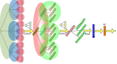
This paper proposes a new graph convolutional neural network architecture based on a depth-based representation of graph structure deriving from quan-tum walks, which we refer to as thequantum-based subgraph convolutional neural network(QS-CNNs). This new architecture captures both the global topologi-cal structure and the lotopologi-cal connectivity structure within a graph. Specifitopologi-cally, we commence by establishing a family ofK-layer expansion subgraphs for each vertex of a graph by quantum walks, which captures the global topological ar-rangement information for substructures contained within a graph. We then design a set of fixed-size convolution filters over the subgraphs, which helps to characterise multi-scale patterns residing in the data. The idea is to apply convo-lution filters sliding over the entire set of subgraphs rooted at a vertex to extract the local features analogous to the standard convolution operation on grid data. Experiments on eight graph-structured datasets demonstrate that QS-CNNs ar-chitecture is capable of outperforming fourteen state-of-the-art methods for the tasks of node classification and graph classification.
Keywords: Graph convolutional neural networks, spatial construction, quantum walks, subgraph.
∗Corresponding author: Lu Bai
Email address: [email protected]. (Lu Bai)
*Manuscript
1. Introduction
Numerous problems (social networks, transport networks, protein-interaction networks, knowledge graphs,. . .) involve data lying on irregular or non-Euclidean space that can be efficiently described with graph data structures, which are uni-versal representations of heterogeneous pairwise relationships [1]. Graphs can
5
encode complex geometric structures and can be studied using efficient machine learning techniques. Recently, numerous results have proven that deep learn-ing methods provide an effective architecture for analyzlearn-ing the large-scale and high-dimensional regular or Euclidean data. In particular, Convolutional Neu-ral Networks (CNNs) [2] allow us to extract meaningful statistical patterns from
10
large sets of data and this property allows them to gain significant improvement in image, sound and video recognition tasks [3], where the underlying data repre-sentation has a regular grid structure. When confronted by graph data-streams, on the other hand, one is confronted with irregular structures. Because such data is ubiquitous, there has been significant interest in the generalization of
15
CNNs to graph data [1]. Unfortunately, this is not a straightforward problem since the basic operations of convolution, pooling and weight-sharing are only designed for regular grids. These three points make the application of CNNs to graph data streams both theoretically and implementally challenging.
There are two main strategies adopted in extending CNNs to non-lattice
20
graphical structures, namely a) spectral and b) spatial methods. Spectral ap-proaches draw on the properties of convolution operators in the graph Fourier domain and are related to the Laplacian matrix of the graph [4, 5, 6]. By trans-forming graphs into the spectral domain using the eigenvectors derived from the eigendecomposition of the graph Laplacian, graphs can be multiplied by an
25
array of filter coefficients to perform a filtering operation. However, spectral approaches require each of the graphs samples in a particular problem to have the same number of nodes. Thus they are not directly transferable to different graphs of different size and having a different Fourier basis.
Spatial approaches, on the other hand, generalize the convolution using the
spatial structure of a graph by sliding a filter over the spatially neighboring ver-tices in a manner analogous to the convolution performed on images in standard CNNs [7, 8, 4, 9, 10]. This approaches however present two challenges, namely (1) the definition of a receptive field/neighborhood, because spatial convolutions are usually position dependent and lack a meaningful global interpretation and
35
(2) how to implement weight sharing in a spatial structure with a variable num-ber of adjacent neighbors adjacent and where the ordering of neighborhoods is not well defined.
To solve these problems, in this paper, we adopt a graph decomposition strat-egy based on quantum walks. When compared to their classical counterparts,
40
quantum walks capture different aspects of the patterns of node connectivity in a graph via constructive and destructive interference. Here we use them to determine the nodes belonging of each receptive field used for convolution in a CNN. This can lead to the convolution operations being performed both more effectively and more efficiently. We commence by decomposing a graph into a
45
family ofK-layer m-ary expansion trees, each rooted at a unique vertex. We then scan a subgraph based window defined over an m-ary tree in a manner similar to the standard convolution operation on grid data (depicted in Figure 1). This allows us to extract structural features reflecting the local connectiv-ity, and this in turn helps in capturing multi-scale patterns in the data. In
50
particular, the convolution operation not only captures local structural infor-mation within the graph, but also exhibits weight sharing among the subgraphs. This results in a significant parameter reduction. The weight sharing is induced by a pooling operation that acts directly on the output of the preceding net-work layer, and without resorting to a preprocessing scheme (e.g., clustering or
55
other techniques). Finally, we can learn a better representation for the purposes of prediction by simultaneously considering both the node features and graph structure information delivered by our subgraph convolution operation.
The remainder of this paper is organized as follows. In Section 2, we present related work and discuss the relationship between our proposed model QS-CNNs
60
Pool
Conv1 Y
FC Conv2
Figure 1: An illustrative example of our QS-CNNs withK = 4 and m = 3. The ‘Conv’
arrow depicts the convolution operation. The subgraph above the ‘Conv’ arrow represents a convolution kernel, extracting structural features along the tree. Then the extracted features are summarized by pooling operation.
that will be used for developing the work presented in this paper. In Section 4, we present a formal definition of the model, including descriptions of graph depth-based representation and graph learning procedures (i.e. subgraph convo-lution and pooling operations). This is followed by an experimental evaluation
65
in Section 5 which explores the performance of QS-CNNs at node and graph classification tasks. Finally, conclusions and directions for future work are pre-sented in Section 6.
2. Related Work
Most of the recent work on extending CNNs to non-lattice graphical
struc-70
tures fall into two broad categories a) spectral and b) spatial approaches.
2.1. Spectral Methods
Spectral approaches provide a well-defined localization operator on graphi-cal data via convolutions in the spectral domain. Spectral graph theory defines
convolutions in terms of an array of filter coefficients multiplied by the graph
75
signals, after transforming the graph signal to a spectral domain representation. Several authors propose graph CNN models that are based on this method of filtering [4, 6, 5]. For instance, Bruna et al. [4] and Henaff et al. [6] used a gener-alization of graph convolutions via the graph Fourier transform. Unfortunately, this involves the computationally expensive multiplication of node features with
80
the eigenvector matrix of the graph Laplacian. Furthermore, computing the re-quired eigenvector matrix is cubic in the number of vertices. To circumvent this problem, Defferrard et al. [11] have proposed an efficient filtering scheme which operates in the spectral domain by using Chebyshev polynomials, and which does not require explicit computation of the Laplacian eigenvectors. Instead, it
85
uses the kth order Chebyshev polynomials of Laplacian eigenvalues as the
pa-rameters of filters that act onk-hop neighbourhoods of the graph. This model was later simplified by Kipf and Welling [12] to use first order polynomials only for the task of semi-supervised nodes classification.
The major drawback of most spectral methods is that they are based on
90
a spectral formulation of the convolution which uses the spectrum of graph Laplacian [13]. It is thus restricted to a fixed and regular graph structure, i.e. the graphs must have the same number of nodes and the nodes must have a fixed degree. This precludes applications on heterogeneous graph datasets, whose structure (number of nodes and nodes degrees) varies from sample to
95
sample. Examples of such heterogeneous data include biochemical datasets. To overcome these limitations of spectral methods, and considering the re-strictions imposed by complexity, we formulate our approach in the spatial do-main by using a depth-based representation of a graph. The do-main challenge here is to define a receptive field over the neighbourhoods and to specify how weights
100
are shared between different local neighbourhoods [4]. Recently, quantum walks have provided a powerful way to solve this challenge. By analogy with a par-ticle propagating on a graph structure, a quantum walk allows different paths interfere with each other in both constructive and destructive manner. This property exponentially speeds up the computation compared to other spectral
algorithms [14, 15]. As a consequence, quantum walkers can reach a vertex through multiple paths, thus the probability of visiting nodes in the neighbour-hoods increases. This leads to the probability of identifying local neighbour structure more effectively and efficiently [16, 17].
2.2. Spatial Methods
110
As mentioned above, spatial approaches have the advantage over spectral approaches in that they can operate on problems where the graph structure varies in the dataset. However, they generally require sophisticated data trans-formations to enable effective learning. Bruna et al. [4] used a spatial method based on multi-scale clustering. Here the required convolutions are defined per
115
cluster, without any weight sharing among neighbourhoods. Duvenaud et al. [9] on the other hand, have proposed a convolution-like propagation rule on graphs. This induces weight sharing among edges. Local filters are applied over neigh-bouring nodes. Another interesting example of a weight-sharing strategy has recently been suggested by Atwood and Towsley [10]. They perform a random
120
walk on the graph in order to select spatially close neighbouring nodes. These nodes are used for the purposes of convolution. Weight sharing is controlled by the number of hops between two nodes. However, the convolution operations underpinning this method are related to the power series of the full transition matrix. Computing this series is computationally expensive, and thus limits its
125
range of applications. In related work, Niepert et al. [7] use a node ordering step which converts graphs locally to a regular 1D grid so that a conventional 1D Euclidean CNN can be used. The main drawback of this method is that the 1D sequences extracted from the graphs discard large amounts of structural information about the detailed arrangement of the nodes. Thus, it does not
130
replicate the standard convolution on regular grids. Moreover, this method [7] is limited since it is only designed for graph classification and does not admit any pooling operations.
In contrast to the previous research, we suggest a novel method which is im-plemented using subgraph convolution and pooling operators that capture both
the global topological and local connectivity structures within the graph. This allows the method to capture multi-scale patterns in the data. We implement the method by applying convolution filters that slide over the entire subgraphs of a vertex. In this way extract local features in a manner similar to the stan-dard convolution operation on grid data. As a result, it induces weight sharing
140
property. Moreover, our method can be applied to the tasks of both node and graphs classification, where pooling operations can be used.
3. Preliminary Concepts
In this section, we introduce some preliminary concepts that will be used for developing the work presented in this paper. To this end, we commence
145
by introducing the background on convolutional neural networks. We then introduce the related basics of graph theory and quantum walks.
3.1. Convolutional Neural Networks
Convolutional neural networks (CNNs) introduce hidden convolution and pooling layers to identify localized features which are independent of spatial
150
location via a set of rectangular filters. The convolution operator scans a set of ‘square’ kernel filters across a grid-structure as input, returning feature maps that represent the response to the filters. Given a multi-channel input, a feature map is the summation of the convolutions with separate kernels for each input channel. In the CNN architecture, the pooling operator is utilized to compress
155
the spatial resolution of each feature map, leaving the number of feature maps unchanged. Applying a pooling operator across a feature map enables the algo-rithm to handle a large number of feature maps and, moreover, it generalizes the feature maps by resolution reduction. Common pooling operations are those of taking the average and the maximum of the receptive cells over the input map
160
[18].
In order to extract input feature effectively for the convolution operation, we need to assume that there exists some locality structure for the spatial arrange-ment of the input. This means that the input signal should be highly correlated
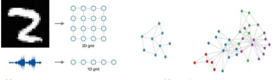
Figure 2: Example of regular grid data and irregular grid data.
over local regions and mostly uncorrelated at a global scale. This works well for
165
data on a regular low-dimensional grid, for instance, images and sound are mod-eled as 2-D grids and 1-D sequences respectively (see Figure 2(a)). However, in many real world problems, the data reside on irregular grids or more generally in non-Euclidean domains. Examples are furnished by social networks, chemical compounds, protein and knowledge graphs, all of which are better structured
170
as a graph (see Figure 2(b)). When confronted by graph data-streams, on the other hand, one is confronted with irregular structures, the basic operations of convolution, pooling and weight-sharing in CNNs, which are only designed for regular grids, are no longer applicable. Therefore, it is necessary to reformu-late the convolution operator on graph structured data. Moreover, to explicitly
175
capture such structures in the data, it may be important and beneficial to inte-grate priors that capture the structure of the mammalian visual cortex into the network architecture [19].
3.2. Graphs
A graphGis a pair of sets (V, E), whereV ={v1, ..., vn}is the set of vertices
180
andE⊆V ×V is the set of edges, formed by pairs of vertices. Each graph can be represented by an adjacency matrixA of sizen×n, wherenis the number of vertices in G. In particular, Ai,j = 1 if there is an edge between vertex vi
sequence of edges and vertices, where the endpoint of each edge are adjacent.
185
A path is a walk in which all vertices are distinct (except possibly the first and last).We denote d(vi, vj) as the length of the shortest path between vertex vi
and vertexvj, and denote k-hop(vi) as the k-neighborhoods of vertexvi, i.e.
d(vi, vj) =k for any verticesvj ofk-hop(vi).
3.3. Quantum Walks
190
Quantum walks have recently emerged as a tool for designing novel algo-rithms on graph structures. They have important properties not exhibited by their classical counterparts [16, 14, 17]. A quantum walk is defined as a dynami-cal process over the vertices of the graph. Moreover, because it is determined by the complex solutions of the Schr¨odinger equation, the continuous time
quan-195
tum walk allows different paths of the walk to interfere with each other in both a constructive and a destructive manner via a complex amplitude. This produces non-classical behavior of quantum walks [20]. While classical walks are ergodic and irreversible, their quantum counterparts are non-ergodic and reversible. As a result, a quantum walk does not approach a steady state with time.
200
The Dirac notation represents the complex amplitudes corresponding to the different states of quantum system using bras and kets. A ket |mi can be interpreted as a column vector, while a bra with the same state label hm| is its conjugate transpose (which is a row vector). We use the Dirac notation to represent the basis state corresponding to the walk being at vertexu ∈ V as
205
|ui. The ket|ψtiis a vector representing the state of the walk at time t , such
that itsu-th entry determines the probability of the walk being at vertexuat timet. A general state of the walk is a complex linear combination of the basis states, which is defined as
|ψti=
X
u∈V
αu(t)|ui (1)
where bothαu(t) and|ψtiare complex numbers, andαu(t)α⋆u(t) gives the
prob-210
ability of finding the walk at the vertex u at time t. ThusPu∈V αu(t)α⋆u(t) = 1
The evolution of the walk is then given by the Schr¨odinger equation, where we denote the time independent Hamiltonian asH
∂
∂t|ψti=−iH|ψti (2)
Given an initial state|ψ0i, the solution for Eq(2) is
215
|ψti=e−iHt|ψ0i (3)
The Hamiltonian operator governs the time evolution of the continuous time quantum walk. It is characterized by a unitary matrix, which renders the walk reversible. In the case where the Hamiltonian is identical to the graph Lapla-cian matrix [21, 22], i.e., H = L, then the structural information residing in the graph is encoded by the Hamiltonian. In the Hilbert space formulation of
220
Quantum Mechanics, the state of a quantum mechanical system associated to the n-dimensional Hilbert space H ∼=Cn is identified with an n×n positive
semidefinite, trace-one, Hermitian matrix, called a density matrix. The Lapla-cian of a graph is symmetric and positive semidefinite. The LaplaLapla-cian of a graph G, scaled by the degree-sum of G, has trace one and it thus has the requested
225
properties of a density matrix.
4. Proposed QS-CNNs Model
In this section we combine the idea of subgraph convolution with that of using a depth-based representation to develop a novel subgraph convolution architecture for a graph. Our idea is to decompose a graph into substructures
230
(i.e., subgraphs) spanned from a root vertex to the remaining vertices with a
K-layer expansion. More specifically, for each vertex, a neighborhood subgraph consisting of exactlymvertices is extracted by quantum walks and normalized as am-ary tree by leveraging graph grafting and graph pruning procedures. The leaf nodes of them-ary tree are further replaced by their own neighbourhood
235
m-ary trees. This process is performed recursively until aK-level m-ary tree is constructed for each vertex. We then construct a set of subgraph feature
detectors, which can be viewed as convolution with a set of finite support kernels. These are computed by sliding the kernels over theK-levelm-ary tree to extract local features, in a manner analogous to that used in the standard convolution
240
operation. After one layer of convolution computations over different positions of the subgraph along the tree structure, structural features are extracted, and a new tree is generated. The new tree has a reduced number of levels when compared with the original input tree. Each parent node and its child nodes in the input layer become a single new node in the next layer. The extracted
245
local features produced by the convolution layer are forwarded to the pooling layer. Thereafter they are packed into one or more fixed-size vectors by taking the max/mean value in each dimension. After the pooling layer, the fixed-size feature vector is subsequently presented to the fully-connected layers (FC) to compute the predicted probability over the class labels. One merit of such an
250
architecture is that each vertex hasK-layer expansion subgraphs. Hence both the a) global topological arrangement information and b) local connectivity structural information contained within a graph can be learned effectively and efficiently by subgraph convolution. This allows our method to capture multi-scale patterns in the data.
255
4.1. The Depth-Based Representation for a Graph
In order to exploit topological information concerning the arrangement of vertices and edges in a graph, we develop aK-layer depth-based representation for a graph. Concretely, the representation comprises two steps: (1) Performing quantum walks on graph for node ranking; (2) Mapping graph to tree: we
260
construct am-ary tree for each vertex in the original graph by leveraging graph grafting and graph pruning procedures. The leaf nodes of thei-levelm-ary tree are replaced by their neighborhoodm-ary trees and thus aK-level m-ary tree is recursively constructed for each vertex.
4.1.1. Quantum Walks on Graph
The fundamental challenge in generalizing CNNs to graph-structured data is to determine the nodes belonging of each receptive field used for convolution while maintaining the shared weights. Recall that the standard convolution operator selects the neighboring pixels of a given pixel and computes the inner product of the weights and these neighbors. We propose a spatial convolution
270
that performs a quantum walk on the graph in order to select the topmclosest neighbors for every node, as shown in Figure 1. The intuition underpinning the use of a quantum walk is that it can capture the global topological arrangement information for substructures contained within a graph. Quantum walks cap-ture different patterns of node connection. Moreover, a quantum walk allows
275
the complex amplitudes corresponding to different paths between two nodes on a graph interfere with each other in both a constructive and a destructive man-ner. Although the classical concepts of hitting and commute time, allow the averaging of path length over the different paths [23] in the case of a quantum walk the effects are more subtle because of the complex nature of the associated
280
amplitude [14]. For instance, if the walk is suitably initialised, then symmetric structure results in a zero amplitude and the amplitude capture long-range as well as local connectivity information [14]. In fact for certain types of sym-metrically structured graphs, quantum walks have exponentially faster hitting times than their classical counterparts [24]. This has obvious benefits in terms
285
of problems involving search on a graph or network.
As a consequence, quantum walkers can reach a vertex simultaneously through multiple paths, and thus at a given time the probability of visiting nodes in the neighbourhoods increases with respect to the classical counterpart. This means that a quantum walker can potentially identify the salient connectivity or
neigh-290
bourhood structure more effectively and efficiently than its classical counterpart.
Given the adjacency matrix A of a graph, the spectral decomposition of the adjacency matrix is A = ΦΛΦT, where Φ = (|ψ
1i,|ψ2i,· · · ,|ψni) is the
n×nmatrix and Λ is the ordered eigenvalue matrix Λ =diag(λ1, λ2,· · · , λn).
According to Eq.(3), we set the initial state Φ0 as Φ and the evolution of the
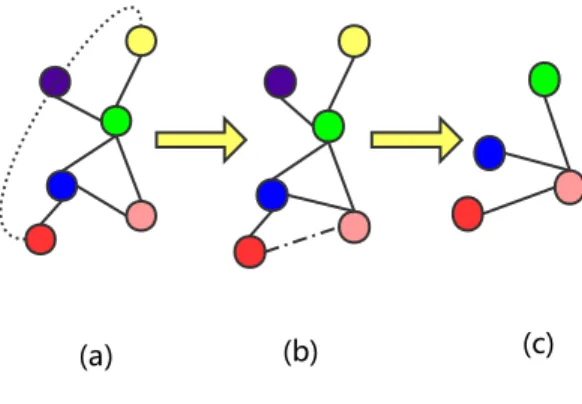
(a) (b) (c)
Figure 3: An illustrative example of graph grafting. Vertices connected in dotted line are the pink vertex’s 2-hop, the red vertex has a higher QW score than other vertices of pink vertex’s 2-hop.
quantum walk on the graph at timetis given by Φt=e−i
Lt
Φ0 (4)
After the above measurement, then×n state matrixAt in quantum walks at timetbecomes
At= ΦtΛΦTt (5)
For every nodeu, we define the quantum walks score (referring to as QW) for the node as
300
QW(u) =X
v∈n
(At)uv (6)
We then sort all the nodes according to their QW scores in descending order.
4.1.2. Mapping Graph to Tree
For each vertex, a receptive field of the same size should be constructed. However, the size of the 1-hops for different nodes are different. To overcome
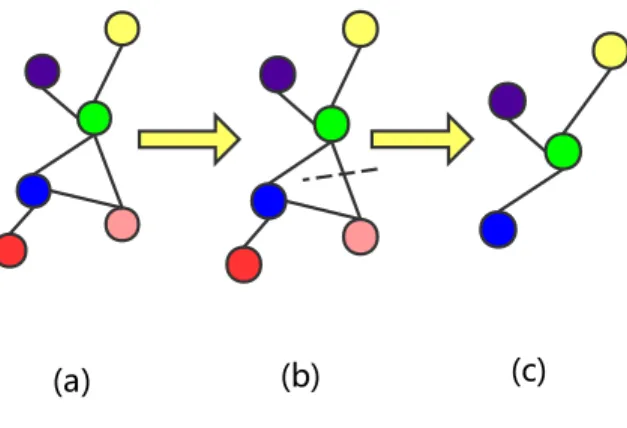
(a) (b) (c)
Figure 4: An illustrative example of graph pruning. The pink vertex has a smaller QW score than other vertices of green vertex’s 1-hop.
this problem, we use graph grafting and graph pruning to standardise the
neigh-305
borhood subgraph for each node to be an m-ary tree.
Graph GraftingFor nodevwhose 1-hop size is less thanm, we use graph grafting to choose nodes from node k-hop(v) (k >=2) to fill node 1-hop(v). As shown in Figure 3, besides the vertex coloured pink itself, we still need to incorporatem= 1 vertex into the receptive field from nodek-hop(v) (k >=2).
310
We commence by selecting nodes from node 2-hop(v). However, if the nodes in the 2-hop are insufficient in number, then we select nodes from the 3-hop and so on. If there exist more nodes than we need, we select nodes with higher QW scores. In this way, the neighborhood subgraph consisting of exactlymvertices is extracted and standardised as anm-ary tree. We then rank the leaf nodes of
315
them-ary tree according to their QW scores.
Graph Pruning For node v whose 1-hop size is greater than m, we use graph pruning to select nodes from node 1-hop(v). As shown in Figure 4, besides the vertex coloured green, we need to cut one node so that onlym= 3 vertices are reserved. We cut nodes with smaller QW scores. In this way,
the neighborhood subgraph consisting of exactly m vertices is extracted and standardised as anm-ary tree. We then rank the leaf nodes of the m-ary tree according to their QW scores.
Using graph grafting and graph pruning, we normalized the subgraph of each node’s as an m-ary tree. The leaf nodes of each m-ary tree are further
325
replaced by their ownm-ary neighborhood trees. In this way, a K-levelm-ary tree is recursively constructed for each vertex. Algorithm 1 gives the steps of the Mapping Graph to Tree algorithm.
Algorithm 1:Mapping Graph to Tree
Input: state matrixAt, receptive field sizem+ 1, the depthK
Output: normalized neighborhood graph (K-levelm-ary tree) for each vertex
1 initialization;
2 compute the QW score for each vertex according to Eq.6;
3 construct am-ary tree with each vertex by the graph grafting and graph
pruning algorithm;
4 fori= 2, i≤K−1 do
5 The leaf nodes of thei-levelm-ary tree are further replaced by their
own neighborhoodm-ary trees;
6 end
7 returnK-levelm-ary tree for each vertex;
4.2. Depth-based Subgraph Convolution Operator
In this section, we first list the notation used in the paper, in Table 1. We
330
then present our depth-based subgraph convolution operator for theK-levelm -ary tree. Figure 1 shows an example of the complete process withK = 4 and
m = 3. In a manner similar to CNNs on images, our QS-CNNs also involves convolution and pooling operations. Our depth-based subgraph convolution operation extracts structural features on the tree. The extracted features are
then summarized by a depth-based subgraph pooling operation. In this way, our QS-CNNs allows effective structural feature learning.
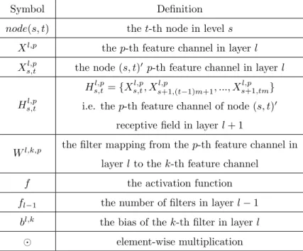
Table 1: Important notations used in this paper and their descriptions.
Symbol Definition
node(s, t) thet-th node in levels
Xl,p thep-th feature channel in layer l
Xs,tl,p the node (s, t) ′
p-th feature channel in layer l
Hs,tl,p Hs,tl,p={X l,p s,t, X l,p s+1,(t−1)m+1, ..., X l,p s+1,tm}
i.e. the p-th feature channel of node (s, t)′
receptive field in layer l+ 1
Wl,k,p the filter mapping from thep-th feature channel in
layerl to thek-th feature channel
f the activation function
fl−1 the number of filters in layerl−1
bl,k the bias of the k-th filter in layerl
⊙ element-wise multiplication
When CNNs are applied to images, a square grid is moved over each image with a particular step size to extract structural features as the output of the convolution. More precisely, a receptive field in the preceding layer becomes a
340
neuron in the next layer after a convolution operation. In this way, the local structural features of images are well captured by the convolution operation. By generalizing CNNs to theK-level m-ary tree obtained in previous steps of graph grafting and graph pruning, we scan a subgraph-based window along the tree to extract structural features as the output of our convolution.
345
The convolutional activation Xs,tl,k for node (s, t), feature k and layer l is
given by Xs,tl,k=f( fXl−1 p=1 ( mX+1 j=1 Wjl,k,pH l−1,p s,t,j ) +b l,k) s≤K−l+ 1
The activationXl,kfork-th feature channel in layerlcan be expressed more
concisely using tensor notation as
Xl,k=f( flX−1
p=1
(Wl,k,p⊙Hl−1,p) +bl,k)
4.3. Depth-based Subgraph Pooling Operator
Another important operation proposed by CNNs is pooling. Reducing the dimensionality of the input data allows the convolution filters to have a large receptive field and at the same time decrease the number of parameters. One of the most common methods for pooling graphs is by performing multi-scale clus-tering of the grid and then performing a pooling operation over each extracted cluster. Instead, our pooling operation acts directly on the output of the pre-ceding layer without any kind of preprocessing scheme. The pooling activation
Xs,tl+1,k for node (s, t), featurekand layer l+ 1 is given by Xs,tl+1,k=f(W
l+1,k·pool(Hl,k s,t) +b
l+1,k)
A maximum pooling function poolmax can be found by taking the maximum value over a region and an average pooling functionpoolavecan be obtained by taking the mean value over a region, thus
poolmax(Rk) =maxi∈Rkai poolavg(Rk) = 1 |Rk| X i∈Rk ai
4.4. Applying QS-CNNs to Node Classification
For the purpose of node classification, each node can be represented by a
K-level m-ary tree constructed through Algorithm 1. After multiple layers of
350
applying the depth-based subgraph convolution and pooling operations, mul-tiple features which carry different structural information constitute the final representationXN of the input node. Then, the final node representation XN
is passed to a fully connected layer and outputs a conditional probability distri-butionP(Y|X), which can be obtained by applying the softmax function. This
355
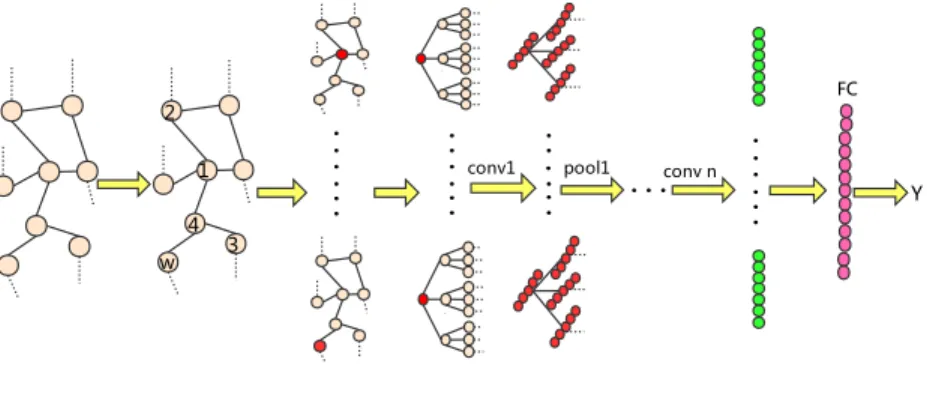
1 2 w 3 4 . . . . . . . . . . . . . . . . . conv1 . pool1 . . .conv n .. . . . . Y FC
Figure 5: Illustration of the proposed QS-CNNs model for graph classification.
P(Y|X) = softmax(f(Wd⊙XN))
4.5. Applying QS-CNNs to Graph Classification
For the graph classification task, we encapsulate a graph by the information conveyed by a set of selected nodes. This potentially allows us to make predic-tions concerning the features of these nodes. We use a node sequence selection
360
algorithm to select a sequence (V) of important nodes. Algorithm 2 illustrates the Node Sequence Selection steps. First, we sort the nodes of the input graph into descending order according to their QW scores. Second, we select the first
W nodes to represent the graph and create a null entry for the node sequence if the number of nodes is smaller thanW.
365
The resulting node sequence is traversed and each visited node is represented by a K-level m-ary tree constructed through the algorithm above if the node value is not 0. Otherwise, we represent the node with aK-levelm-ary tree, with all node values set to zero. After multiple depth-based subgraph convolution and pooling operations simultaneously have acted on theseK-levelm-ary trees, we obtain the feature map XG of the graph. The architecture is completed by a dense layer that connects XG to predict Y. A conditional probability
Algorithm 2:Node Sequence Selection
Input: QW scores for all nodes, widthW
Output: selected node sequenceV
1 initialization;
2 sort (descend) the nodes of the input graph using the given QW scores to
getVsort;
3 if |Vsort|>=W then
4 V = the firstW elements ofVsort 5 else
6 V =VsortandW − |Vsort| dummy nodes 7 end
8 returnselected node sequenceV;
distributionP(Y|X) can be obtained by applying the softmax function:
P(Y|X) = softmax(f(Wd⊙XG))
A generic illustration of the proposed QS-CNNs architecture for graph clas-sification is shown in Figure. 5. It is important to note that our depth-based convolutional representation for the graph is invariant with respect to the per-mutation of node index (rather than the node position). This means that the activations of two isomorphic input graphs will be the same. We prove it as
370
follows.
Theorem 1. The depth-based convolutional activations of two isomorphic input graphs will be the same.
Proof. We prove this theorem by contradiction.
Assume two graphsG1 and G2 are isomorphic but their depth-based
convolu-tional activations are different. At least a pair of nodesu, w, whereu,v belongs to the resulting node sequence of graphG1 and G2 respectively and will have
the same position in the resulting node sequence. The activations ofuand v
can be written as Xul,k=f( fXl−1 p=1 (Wul,k,p⊙H l−1,p u ) +b l,k u ) Xl,k v =f( fXl−1 p=1 (Wl,k,p v ⊙H l−1,p v ) +b l,k v ) Note that Wul,k,p=W l,k,p v =W l,k,p bl,k u =b l,k v =b l,k
Graphs that are isomorphic (the same except for vertex labels) become identical after canonical graph labeling, so
Hl−1,p
u =Hvl−1,p=Hl−1,p
by isomorphism, allowing us to rewrite the activation as
Xul,k=f( fXl−1 p=1 (Wl,k,p⊙Hl−1,p) +bl,k) Xl,k v =f( fXl−1 p=1 (Wl,k,p⊙Hl−1,p) +bl,k)
Which implies thatXl,k
u =Xvl,kand presents a contradiction and completes the
proof.
375
4.6. Learning Filters
We assume that each convolution layerlis followed by a pooling layerl+ 1. According to the back propagation algorithm, in order to compute the sensitivity for a unit at layerl, we should first sum over the sensitivities of the next layer corresponding to units that are connected to the node of interest in the current layerl. We multiply each of these connections by the associated weights defined at layerl+ 1. We then multiply this quantity by the derivative of the activation function evaluated at the pre-activation inputs of the current layerZ. In the case of a convolutional layer followed by a pooling layer, we can upsample the pooling
layers sensitivity mapδl+1,k to make it the same size as the convolutional layer
map. Then we perform elementwise multiplication of the upsampled sensitivity map from layerl+ 1 with the activation derivative map at layerl. The ‘weights’ defined at a pooling layer map are all equal toWl,k, snd so we simply scale the
previous step result by Wl,k to complete the computation of δl,k. So we can
get: δl,k , ∂E ∂Zl,k δl,k= ∂E ∂Zl+1,k · ∂Zl+1,k ∂X1,k · ∂Xl,k ∂Z1,k δl,k=f′ (Zl)⊙(up(Wl+1,kδl+1,k)) δl,k=Wl+1,k(f′ (Zl)⊙up(δl+1,k))
where up is the Upsampling function and E is the loss energy. Finally, the gradients for the kernel weights are computed using back propagation:
∂E ∂Wl,k,p = X i,j (δl,k)i,j(Pl−1,p)i,j where (Pl−1,p)
i,j is the patch in Xl−1,p that was multiplied element-wise by Wl,k,pduring convolution. we can compute the bias gradient by simply summing
over all the entries inδl,k: ∂E ∂bl,k = X i,j (δl,k) i,j
5. Experiments and Comparisons
In this section, we experimentally investigate the merits and limitations of the proposed QS-CNNs model, including its computational complexity and pa-rameter determination. A comprehensive experimental study on a variety of
380
data sets is conducted in order to compare our proposed model QS-CNNs with several state-of-art methods for node classification and graph classification tasks.
In this section, we denote a graph convolution layer withkfeature maps byCk
and a fully connected layer withk hidden units byF Ck. In addition, lr stands
for the learning rate, L2 denotes the L2 regularization parameter and dropout
385
5.1. Node Classification
To demonstrate the effectiveness of the proposed approach on the node clas-sification task, we conduct experiments on two citation network datasets and one data set arising from e-mail communications in a social network. These
390
are respectively the Cora, Pubmed datasets [25] and the Email-Eu dataset [26]. Each citation dataset consists of scientific papers (represented by nodes), cita-tion links (represented by edges), and topics or subjects (represented by labels). Table. 2 summarizes the coverage and properties of the three data sets. For node classification, six alternative algorithms are selected as baseline
compara-395
tors. We briefly describe these methods in turn.
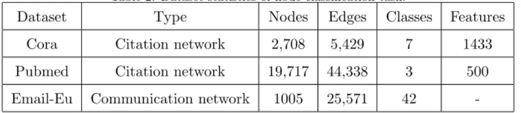
Table 2: Dataset statistics of node classification task.
Dataset Type Nodes Edges Classes Features
Cora Citation network 2,708 5,429 7 1433
Pubmed Citation network 19,717 44,338 3 500
Email-Eu Communication network 1005 25,571 42
-DatasetsThe Cora dataset [25] contains 2,708 machine learning articles cat-egorized into seven possible machine learning subject or topic classes. Each article is represented by a binary 0/1-valued word vector where each feature
400
corresponds to the presence or absence of a term drawn from a dictionary. The dictionary contains 1,433 unique entries. This graph contains 5,429 citation edges. We treat the citation links as undirected edges and construct a binary, symmetric adjacency matrix.
The Pubmed dataset [25] consists of 19,717 scientific papers from the Pubmed
405
database on the subject of diabetes. Each paper is classified into one of three classes. This citation network that links the papers consists of 44,338 links. Each paper is represented by a Term Frequency Inverse Document Frequency (TFIDF) vector drawn from a dictionary with 500 terms. As with the CORA corpus, we construct an adjacency-based QS-CNNs that treats the citation
work as an undirected graph.
The Email-Eu dataset [26] was generated using email data from a large Eu-ropean research institution. There is an edge (u, v) in the network if person
usent personv at least one email. The e-mails only represent communication between institution members. The dataset also contains ”ground-truth”
com-415
munity memberships of the nodes. Each individual belongs to exactly one of 42 departments at the research institute. Note that the vertices of the Email-Eu-Core have no vertex information, so we only take the structural information of the vertices as the input.
420
Baseline MethodsWe compare our proposed method QS-CNNs with six state-of-the-art methods for node classification. The methods used for comparisons are (1) ℓ1-regularized logistic regression (l1logistic), (2) ℓ2-regularized logistic regression (l2logistic), (3) exponential diffusion kernels-on-graphs (KED) [25], (4) Laplacian exponential diffusion kernels-on-graphs (KlED) [25], (5) diffusion
425
convolutional neural networks (DCNNs) [10], (6) GraphSAGE [27]. For the ‘l1logistic’ and ‘l2logistic’ methods, we use node features alone as the input for logistic regression. This means that graph structure information is not consid-ered, and the regularization parameter is fine tuned by the validation set. For ‘KED’ and ‘KlED’ , we take the graph structure as input, which means that node
430
feature information is not considered. Similar to previous work [10], we chose parameters for various baseline methods as follows: a) the penalty for l1logistic and l2logistic is chosen from the set{10−4,10−3, ...,103,104}, b) the parameter
αfor ‘KED’ and ‘KlED’ is chosen from the set{10−6,10−5, ...,102}, c) the
pa-rameterH = 2 is used for DCNNs because it results in the best classification
435
accuracy, d) GraphSAGE provides a variety of alternative approaches for ag-gregating features within a sampled neighborhood, and we choose GraphSAGE-mean because it almost always results in the best accuracy. For each baseline method, we report the results for the parameters which give the best classifica-tion accuracy.
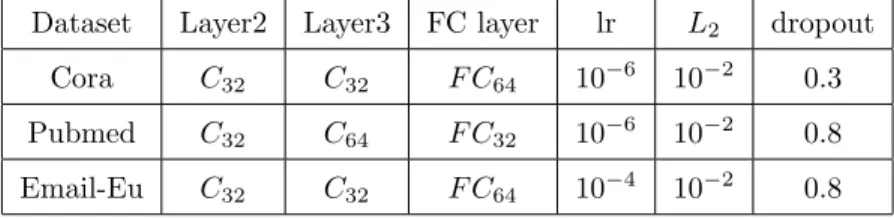
Table 3: The details of some parameters for node classification.
Dataset Layer2 Layer3 FC layer lr L2 dropout
Cora C32 C32 F C64 10−6 10−2 0.3
Pubmed C32 C64 F C32 10−6 10−2 0.8
Email-Eu C32 C32 F C64 10−4 10−2 0.8
Experimental Set-upFor all datasets, we standardize each node as a 3 level 3-ary tree. We train a five-layer QS-CNNs, where the first layer is the input layer, the second and third layers are the convolutional layer, the fourth layer is the fully-connected layer, and the final layer is the output layer. We use
445
the Adam optimization algorithm [28] for gradient descent. All weights are randomly initialized from a normal distribution with mean zero and variance 0.01. We choose ReLU as the activation function. This model was implemented in Python using tensorflow [29]. A 10-fold cross-validation strategy is employed to evaluate the classification performance. Specifically, the entire sample is
450
randomly partitioned into 10 subsets and then we choose one subset for test and use the remaining 9 for training, and this procedure is repeated 10 times. The final accuracy is computed by averaging the accuracies from each of the random subsets.
Network Configuration For node classification, our QS-CNNs has 3
para-455
metric layers. Its configuration for different datasets are as follows: a) for Cora:
C32−C32−F C64, 10−6(learning rate), 10−2(L2 regularization) and 0.3 (dropout rate); b) for Pubmed: C32−C64−F C32, 10−6 (learning rate), 10−2 (L2 reg-ularization) and 0.8 (dropout rate); and c) for Email-Eu: C32−C32−F C64, 10−4 (learning rate), 10−2 (L2 regularization) and 0.8 (dropout rate). These
460
properties can be found in Table 3.
Results DiscussionTable. 4 reports the average classification accuracy of the different algorithms on node classification. The boldfaced values are the best result in each row. Our proposed five-layer QS-CNNs outperforms each of the
Table 4: Study of node classification: classification accuracy (in MEAN±STD). A comparison
of the performance between six baseline methods and our proposed QS-CNNs on three node classification datasets. The QS-CNNs offers the best performance. - means the model is not suitable for the data set.
Model Cora Pubmed Email-Eu
l1logistic 71.63±0.71 87.68 ±0.89 -l2logistic 71.81±0.69 86.54 ±0.93 -KED 81.92±0.91 83.15 ±0.64 70.28±0.87 KlED 83.27±0.76 84.11 ±0.77 71.54±0.81 DCNN 82.52±2.11 88.57 ±1.34 -GraphSAGE 82.68±1.83 88.41 ±1.25 73.59±1.72 DS-CNNs 84.72±2.28 89.63±1.67 76.61±2.33 QS-CNNs 85.95 ± 1.58 89.63 ±1.67 77.63 ±1.94
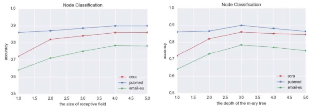
Figure 6: Impact of the receptive field size and the depth of them-ary tree on performance
competing methods for all datasets studied and the improvement is in the range from 2.68% to 14.32% on the Cora dataset, from 1.06% to 6.48% on the Pubmed dataset and from 4.04% to 7.35% on the Email-Eu dataset respectively. On the Cora dataset, l1logistic and l2logistic give the worst performance. This may be explained by the fact that the logistic regression models only take the node
470
features as input and neglect graph structure information. KED and KLED both take graph structure as input (e.g. node features are not used) and show inferior performance to our QS-CNNs. This indicates that our QS-CNNs is able to extract graph structure features. On the Pubmed dataset, we observed that those methods which incorporate node features outperform those methods that
475
do not, i.e., l1logistic and l2logistic are superior to both KED and KLED in terms of accuracy. Furthermore, our QS-CNNs still maintains the best classi-fication accuracy. Our QS-CNNs outperforms GraphSAGE-mean (taking the elementwise mean value of feature vectors) suggesting that assigning different weights to different nodes within a subgraph while dealing with differently sized
480
neighbourhoods may be beneficial. Based on these results, it is demonstrated that our proposed method QS-CNNs integrates the merits of using both the global topological and local connectivity structures within a graph. Thus, it performs better than the traditional methods.
To investigate the effect of different receptive field size ofm+1 and the depth
485
K of the m-ary tree on the node classification performance of our proposed method QS-CNNs, we test several values of m+ 1 and K. We report the results in Figure 6, in which we plot the classification accuracies of our QS-CNNs method versus m+ 1 and K respectively. The different coloured lines represent the results on the different datasets. The classification accuracies tend
490
to increase with increasing values ofm+ 1 andK. This is because the greater the values ofm+ 1 and K, the more global topological and local connectivity information can be captured using our QS-CNNs method.
5.2. Graph Classification
To demonstrate the effectiveness of the proposed approach on graph
classi-495
fication, we conduct experiments on five benchmark data sets abstracted from bioinformatics databases, i.e., a) MUTAG [30], b) PTC [31], c) NCI1 [32], d) D&D [33], and e) PROTEINS [34]. Information concerning the properties of these datasets is listed below and summarized in Table. 5. For graph classi-fication, eight alternative algorithms are selected as baselines. We will briefly
500
detail these methods in turn.
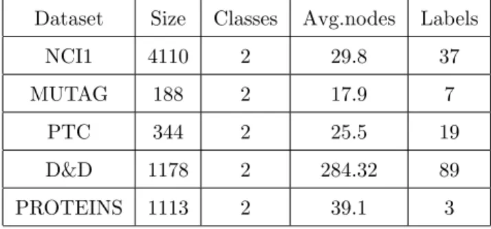
Table 5: Dataset statistics for graph classification task.
Dataset Size Classes Avg.nodes Labels
NCI1 4110 2 29.8 37
MUTAG 188 2 17.9 7
PTC 344 2 25.5 19
D&D 1178 2 284.32 89
PROTEINS 1113 2 39.1 3
DatasetsThe NCI1 [32] dataset made publicly available by the National Cancer Institute (NCI) is a subset of balanced datasets of chemical compounds screened for the ability to suppress or inhibit the growth of tumours. It consists of 4100
505
graphs that represent chemical compounds and each node is assigned one of 37 possible labels. MUTAG [30] is a data set of 188 nitro compounds where the class label is as either aromatic or heteroaromatic with seven node features. PTC [31] comprises 344 compounds where the class label indicates whether they are carcinogenic or not in rats with 19 node features. D&D is a data set of 1178
510
protein structures obtained from [33], classified into enzymes and non-enzymes. Each protein is represented as a graph whose nodes correspond to amino acids and two nodes are linked by an edge if they are less than 6 ˚Angstroms apart. PROTEINS is a dataset obtained from [34] where these nodes are secondary structure elements and there is an edge between two nodes if they are
bours in the amino-acid sequence or in 3D space. It has 3 discrete labels, which represent helix, sheet or turn.
Baseline Methods We compare our proposed method QS-CNNs with eight state-of-the-art methods for graph classification. These methods are used for
520
comparisons are (1) the Weisfeiler-Lehman subtree kernel (WL) [35], (2) the random walk kernel (RW) [36], (3) the shortest-path kernel (SP) [37], (4) the graphlet count kernel (GK) [38], (5) the PATCHY-SAN method which combin-ing receptive fields for nodes and edges uscombin-ing a merge layer k = 10E
(PSCN-10E) [7], (6)p-step random-walk kernel (p-RW) [39], (7) Ramon-G¨artner kernels
525
(RG) [40], (8) FGSD[41]. In accordance with established [42], the decay fac-tor for random-walk is chosen from{10−6,10−5, . . . ,10−1}, the pvalue in the
p-step random-walk kernel is chosen from {1,2, . . . ,10}, the height parameter in Ramon-G¨artner subtree kernel is chosen from{1,2,3}. For each kernel, we report the results for the parameters which give the best classification accuracy.
530
For Weisfeiler-Lehman subtree kernel, we set the height parameterh= 2 for it could increase the feature space exponentially. For the graphlet kernel, we set the size of the graphletskto 7 since it could exhibit the sparsity problem. We set the parameterk = 10E for PSCN becasue a receptive size of 10 results in
the best classification accuracy and the result is quoted from [7]. For FGSD,
535
the parameters are set the same as [41].
Experimental Set-up For the NCI1 dataset, we set width W=25 (W rep-resents the number of selected nodes from each graph), and standardize each vertex as a 3 level 9-ary tree. We train a six-layer QS-CNNs, where the first
540
layer is the input layer, the second, third and fourth layers are the convolu-tional layer, the fifth layer is the fully-connected layer, and the final layer is the output layer. For the remaining datasets, we set the width W=15, and again standardize each vertex as a 3 level 9-ary tree, but instead, we train a five-layer QS-CNNs, where the second and third layers are the convolutional layer, the
545
Table 6: The details of some parameters for graph classification.
Dataset Layer2 Layer3 Layer4 FC lr L2 dropout
NCI1 C32 C32 C64 F C32 5·10−3 10−2 0.8
MUTAG C32 C32 - F C64 10−2 10−2 1
PTC C32 C32 - F C64 10−2 10−2 1
D&D C32 C32 - F C64 10−2 10−2 1
PORTEINS C32 C32 - F C64 10−2 10−2 1
Table 7: Study of graph classification: classification accuracy (in MEAN±STD). A
compar-ison of the performance between eight baseline methods and our proposed QS-CNNs on five graph classification datasets. The last column shows the averaged classification accuracy of all the algorithms over the five datasets. The QS-CNNs offers the best performance.
Algorithm NCI1 MUTAG PTC PROTEIN D&D AVG
WL 80.22±0.51 80.71±0.31 56.77±2.11 72.92±0.56 77.95±0.7 73.71±0.84 RW >72h 83.73±1.51 57.85±1.30 74.22±0.42 >72h -SP 73.00±0.24 85.22±2.43 58.24±2.44 75.07±0.54 >72h -GK 62.28±0.29 81.66±2.11 57.26±1.41 71.67±0.55 78.45±0.26 70.26±0.92 p-RW >72h 80.05±1.64 59.38±1.66 71.16±0.35 >72h -RG 56.61±0.53 84.88±1.86 59.47±1.66 70.73±0.35 >72h -PSCN-10E 78.59±1.89 92.63±4.21 60.00±4.82 75.89±2.76 77.12±2.41 76.85±3.22 FGSD 79.80±2.36 92.12±3.98 62.80±4.07 73.42±3.42 77.10±2.78 76.46±3.25 DS-CNNs 80.12±2.87 92.87±4.81 64.67±5.00 78.35±4.00 79.22±4.06 79.05±4.15 QS-CNNs 81.43±2.56 93.13±4.67 65.99±4.43 78.80±4.63 81.41±3.46 80.15±3.95
algorithm [28] for gradient descent. The initial values of weights, the type of activation function and the implementation environment are set in the same manner as for node classification. We again adopt a 10-fold cross-validation strategy as described above.
550
Network ConfigurationFor graph classification, we used the following sets of hyperparameters a) for MUTAG, PTC, D&D and PORTEINS:C32−C32−F C64, 10−2(learning rate), 10−2(L2 regularization) and 1 (dropout rate); b) for NCI1:
C32−C32−C64−F C32, 5·10−3 (learning rate), 10−2 (L2 regularization) and
555
0.8 (dropout rate). These properties can be found in Table 6.
Figure 7: Impact of the receptive field size and the depth of them-ary tree on the performance
for graph classification
methods are shown in Table 7, in which the boldfaced values again indicate the best result in each row. Again, we observe that our proposed method QS-CNNs
560
outperforms the alternative for all five datasets. The last column of Table. 7 shows the averaged classification accuracy over all the algorithms tested for the five datasets. Note that, some kernels cannot complete the kernel matrix computation on some of the datasets. For these kernels, we perform the sta-tistical analysis on those datasets on which the computation can be completed.
565
Our method has improved the classification accuracy by 6.44% (WL), 9.89% (GK), 3.3% (PSCN-10E) and 3.69% (FGSD) respectively, compared to the
av-eraged classification of all competing methods over the five datasets. Moreover, our QS-CNNs performs better than the PSCN-10E algorithm, although they
are both have a CNN architecture. The main reason is that the PSCN-10E
570
[7] uses node ordering step which converts graphs locally to a regular 1D grid hence discarding a large amount of the structural information residing in the graphs. Our proposed QS-CNNs is fundamentally different from most existing graph CNNs framework, where each vertex hasK-layer expansion subgraphs, and hence structural information can be learned effectively and efficiently by
575
subgraph convolution. Thus, it is capable of revealing both the global topolog-ical and local connectivity structures for a graph. The relatively high standard deviations can be explained by the small size of the benchmark datasets and the
fact that we normalize each node neighbourhood as the same 3 level 9-ary tree for different datasets. Finally, as with node classification, we evaluate how the
580
graph classification accuracies vary with increasing receptive field size ofm+ 1 and the depth K of the m-ary tree. Figure 7 gives the classification results. The results show that with increasingm+ 1 andK, the classification accuracy first increases to a maximum value (i.e., atm+ 1 = 4 andK= 3) and then de-creases slightly, finally reaching a steady state. This observation further verifies
585
the effectiveness of our proposed method QS-CNNs which integrates both global topological arrangement information and local connectivity properties within a graph to conduct graph convolution.
5.3. The Effect of Quantum Walks
Finally, in order to study the contribution of quantum walks in terms of its
590
impact on final classification accuracy, we ran experiments by replacing quantum walks with random walk (referred to as DS-CNNs) and keep the pruning and grafting trick. The results are shown in Table. 4 and Table. 7. As can be observed, QS-CNNs is superior to DS-CNNs in terms of accuracy values for all datasets studied. Meanwhile, QS-CNNs gives a lower standard deviation and
595
hence more stable than the DS-CNNs. It is demonstrated that quantum walks can identify local neighbor structure of nodes more effectively and efficiently.
6. Conclusions and Future Work
In this paper, we have shown how to construct quantum-based subgraph convolution network for a graph. The convolution process makes use of both
600
the global topological arrangement information and local connectivity struc-tures within a graph. Experimental results on node classification and graph classification show our QS-CNNs is superior to a number of baseline methods.
Our future plans are to extend the work in a number of ways. First, in prior work, we have developed methods for characterizing graphs using the commute
605
methods encapsulate the path length distribution between vertices. It would be interesting to use the commute time or heat kernel as a means of node ordering. Second, the current formulations of graph convolution are restricted to use ver-tex information and do not make use of edge labels. It would be interesting to
610
design convolution operation which simultaneously learns properties from both graph vertices and edges. Finally, in [44], Brabandere et al. proposed dynamic filter networks, to define a subnetwork, taking the preceding feature maps as input and generating data-adaptive convolutional filters that can be applied to the preceding feature maps. It would be interesting to use such a subnetwork
615
to determine the local filters dynamically for each specific input subgraph. This may provide a more meaningful interpretation concerning the graph structure by the means of filter generating networks.
Acknowledgment
This work is supported by National Natural Science Foundation of China
620
(Grant Nos.61402389, 61503422 and 11401499), the Natural Science Founda-tion of Fujian Province of China (Grant No.2015J05016) and the Fundamental Research Funds for the Central Universities in China (no. 20720160073).
References
[1] M. M. Bronstein, J. Bruna, Y. LeCun, A. Szlam, P. Vandergheynst,
625
Geometric learning: going beyond euclidean data, arXiv preprint
arXiv:1611.08097.
[2] Y. LeCun, L. Bottou, Y. Bengio, P. Haffner, Gradient-based learning ap-plied to document recognition, Proceedings of the IEEE 86 (11) (1998) 2278–2324.
630
[3] Y. LeCun, Y. Bengio, G. Hinton, Deep learning, Nature 521 (7553) (2015) 436–444.
[4] J. Bruna, W. Zaremba, A. Szlam, Y. LeCun, Spectral networks and locally connected networks on graphs, arXiv preprint arXiv:1312.6203.
[5] O. Rippel, J. Snoek, R. P. Adams, Spectral representations for
convolu-635
tional neural networks, in: Advances in Neural Information Processing Systems, 2015, pp. 2449–2457.
[6] M. Henaff, J. Bruna, Y. LeCun, Deep convolutional networks on graph-structured data, arXiv preprint arXiv:1506.05163.
[7] M. Niepert, M. Ahmed, K. Kutzkov, Learning convolutional neural
net-640
works for graphs, in: Proceedings of The 33rd International Conference on Machine Learning, 2016, pp. 2014–2023.
[8] J.-C. Vialatte, V. Gripon, G. Mercier, Generalizing the convolution opera-tor to extend cnns to irregular domains, arXiv preprint arXiv:1606.01166. [9] D. K. Duvenaud, D. Maclaurin, J. Iparraguirre, R. Bombarell, T. Hirzel,
645
A. Aspuru-Guzik, R. P. Adams, Convolutional networks on graphs for learning molecular fingerprints, in: Advances in neural information pro-cessing systems, 2015, pp. 2224–2232.
[10] J. Atwood, D. Towsley, Diffusion-convolutional neural networks, in: Ad-vances in Neural Information Processing Systems, 2016, pp. 1993–2001.
650
[11] M. Defferrard, X. Bresson, P. Vandergheynst, Convolutional neural net-works on graphs with fast localized spectral filtering, in: Advances in Neu-ral Information Processing Systems, 2016, pp. 3837–3845.
[12] T. N. Kipf, M. Welling, Semi-supervised classification with graph convolu-tional networks, arXiv preprint arXiv:1609.02907.
655
[13] D. I. Shuman, S. K. Narang, P. Frossard, A. Ortega, P. Vandergheynst, The emerging field of signal processing on graphs: Extending high-dimensional data analysis to networks and other irregular domains, IEEE Signal Pro-cessing Magazine 30 (3) (2013) 83–98.
[14] D. Emms, R. C. Wilson, E. R. Hancock, Graph matching using the
in-660
terference of continuous-time quantum walks, Pattern Recognition 42 (5) (2009) 985–1002.
[15] F. Zhang, E. R. Hancock, Graph spectral image smoothing using the heat kernel, Pattern Recognition 41 (11) (2008) 3328–3342.
[16] L. Bai, L. Rossi, A. Torsello, E. R. Hancock, A quantum jensen–shannon
665
graph kernel for unattributed graphs, Pattern Recognition 48 (2) (2015) 344–355.
[17] J. Wang, R. C. Wilson, E. R. Hancock, Spin statistics, partition functions and network entropy, Journal of Complex Networks 5 (6) (2017) 858–883. [18] Y.-L. Boureau, J. Ponce, Y. LeCun, A theoretical analysis of feature pooling
670
in visual recognition, in: Proceedings of the 27th international conference on machine learning, 2010, pp. 111–118.
[19] Y. Bengio, A. Courville, P. Vincent, Representation learning: A review and new perspectives, IEEE transactions on pattern analysis and machine intelligence 35 (8) (2013) 1798–1828.
675
[20] L. Rossi, A. Torsello, E. R. Hancock, Measuring graph similarity through continuous-time quantum walks and the quantum jensen-shannon diver-gence, Physical Review E 91 (2) (2015) 022815.
[21] S. L. Braunstein, S. Ghosh, S. Severini, The laplacian of a graph as a density matrix: a basic combinatorial approach to separability of mixed
680
states, Annals of Combinatorics 10 (3) (2006) 291–317.
[22] F. Passerini, S. Severini, Quantifying complexity in networks: the von neu-mann entropy, International Journal of Agent Technologies and Systems (IJATS) 1 (4) (2009) 58–67.
[23] H. Qiu, E. R. Hancock, Clustering and embedding using commute times,
685
[24] J. Kempe, Quantum random walks hit exponentially faster, arXiv preprint quant-ph/0205083.
[25] P. Sen, G. Namata, M. Bilgic, L. Getoor, B. Galligher, T. Eliassi-Rad, Collective classification in network data, AI magazine 29 (3) (2008) 93.
690
[26] H. Yin, A. R. Benson, J. Leskovec, D. F. Gleich, Local higher-order graph clustering, in: Proceedings of the 23rd ACM SIGKDD International Con-ference on Knowledge Discovery and Data Mining, ACM, 2017, pp. 555– 564.
[27] W. L. Hamilton, R. Ying, J. Leskovec, Inductive representation learning
695
on large graphs, in: Neural Information Processing Systems (NIPS), 2017. [28] D. Kingma, J. Ba, Adam: A method for stochastic optimization, arXiv
preprint arXiv:1412.6980.
[29] M. Abadi, A. Agarwal, P. Barham, E. Brevdo, Z. Chen, C. Citro, G. S. Corrado, A. Davis, J. Dean, M. Devin, et al., Tensorflow: Large-scale
700
machine learning on heterogeneous distributed systems, arXiv preprint arXiv:1603.04467.
[30] A. K. Debnath, R. L. Lopez de Compadre, G. Debnath, A. J. Shusterman, C. Hansch, Structure-activity relationship of mutagenic aromatic and het-eroaromatic nitro compounds. correlation with molecular orbital energies
705
and hydrophobicity, Journal of medicinal chemistry 34 (2) (1991) 786–797. [31] H. Toivonen, A. Srinivasan, R. D. King, S. Kramer, C. Helma, Statistical evaluation of the predictive toxicology challenge 2000–2001, Bioinformatics 19 (10) (2003) 1183–1193.
[32] N. Wale, I. A. Watson, G. Karypis, Comparison of descriptor spaces for
710
chemical compound retrieval and classification, Knowledge and Information Systems 14 (3) (2008) 347–375.
[33] P. D. Dobson, A. J. Doig, Distinguishing enzyme structures from non-enzymes without alignments, Journal of molecular biology 330 (4) (2003) 771–783.
715
[34] K. M. Borgwardt, C. S. Ong, S. Sch¨onauer, S. Vishwanathan, A. J. Smola, H.-P. Kriegel, Protein function prediction via graph kernels, Bioinformatics 21 (suppl 1) (2005) i47–i56.
[35] N. Shervashidze, P. Schweitzer, E. J. v. Leeuwen, K. Mehlhorn, K. M. Borgwardt, Weisfeiler-lehman graph kernels, Journal of Machine Learning
720
Research 12 (Sep) (2011) 2539–2561.
[36] T. G¨artner, P. Flach, S. Wrobel, On graph kernels: Hardness results and efficient alternatives, in: In Proceedings of the 16th Annual Conference on Learning Theory and Kernel Machines, Springer, 2003, pp. 129–143. [37] K. M. Borgwardt, H.-P. Kriegel, Shortest-path kernels on graphs, in: In
725
Proceedings of the 15th IEEE International Conference on Data Mining, IEEE, 2005, pp. 74–81.
[38] N. Shervashidze, S. Vishwanathan, T. Petri, K. Mehlhorn, K. Borgwardt, Efficient graphlet kernels for large graph comparison, in: Artificial Intelli-gence and Statistics, 2009, pp. 488–495.
730
[39] A. J. Smola, R. Kondor, Kernels and regularization on graphs, in: Learning theory and kernel machines, Springer, 2003, pp. 144–158.
[40] J. Ramon, T. G¨artner, Expressivity versus efficiency of graph kernels, in: Proceedings of the first international workshop on mining graphs, trees and sequences, 2003, pp. 65–74.
735
[41] S. Verma, Z.-L. Zhang, Hunt for the unique, stable, sparse and fast feature learning on graphs, in: Advances in Neural Information Processing Systems 30, 2017, pp. 87–97.
[42] P. Yanardag, S. Vishwanathan, Deep graph kernels, in: Proceedings of the 21th ACM SIGKDD International Conference on Knowledge Discovery and
740
Data Mining, ACM, 2015, pp. 1365–1374.
[43] B. Xiao, E. R. Hancock, R. C. Wilson, Graph characteristics from the heat kernel trace, Pattern Recognition 42 (11) (2009) 2589–2606.
[44] B. De Brabandere, X. Jia, T. Tuytelaars, L. Van Gool, Dynamic filter networks, in: Neural Information Processing Systems (NIPS), 2016.
Zhihong Zhang
received his BSc degree (1st class Hons.) in computer
science from the University of Ulster, UK, in 2009 and the PhD degree in
computer science from the University of York, UK, in 2013. He won the K.
M. Stott prize for best thesis from the University of York in 2013. He is
now an associate professor at the software school of Xiamen University,
China. His research interests are wide-reaching but mainly involve the
areas of pattern recognition and machine learning, particularly problems
involving graphs and networks.
Dongdong Chen
is now a master student at the software school of
Xiamen University, China. His research interests include data mining,
machine learning, and network representation learning.
Jianjia Wang
received the B.Sc. degree from Nanjing University of Posts
and Telecommunications (2011) and M.Sc. degrees from Hong Kong
University of Science and Technology (2013). He worked as a research
assistant at Hong Kong Applied Science and Technology Research
Institute from 2013 to 2014. He is currently pursuing the Ph.D. degree in
the Department of Computer Science, University of York, U.K. His
research interests include statistical pattern recognition, complex
networks, information theory, thermodynamic and quantum statistics,
especially in graph and network analysis.
Lu Bai
received the Ph.D. degree from the University of York, York, UK,
and both the B.Sc. and M.Sc degrees from Faculty of Information
Technology, Macau University of Science and Technology, Macau SAR, P.R.
China. He is now a Associate Professor in School of Information, Central
University of Finance and Economics, Beijing, China. His current research
interests include structural pattern recognition, machine learning,
quantum walks on networks and graph matching, especially in kernel
methods and complexity analysis on (hyper)graphs and networks.
Edwin R. Hancock
holds a BSc degree in physics (1977), a PhD degree in
high-energy physics (1981) and a D.Sc. degree (2008) from the University
of Durham, and a
doctorate Honoris Causa
from the University of
Alicante in 2015. From 1981-1991 he worked as a researcher in the fields
of high-energy nuclear physics and pattern recognition at the
Rutherford-Appleton Laboratory (now the Central Research Laboratory
providing the first measurements of charmed particle lifetimes. He also
held adjunct teaching posts at the University of Surrey and the Open
University. In 1991, he moved to the University of York as a lecturer in
the Department of Computer Science, where he has held a chair in
Computer Vision since 1998. He leads a group of some 25 faculty,
research staff, and PhD students working in the areas of computer vision
and pattern recognition. His main research interests are in the use of
optimization and probabilistic methods for high and intermediate level
vision. He is also interested in the methodology of structural and
statistical and pattern recognition. He is currently working on graph
matching, shape-from-X, image databases, and statistical learning theory.
His work has found applications in areas such as radar terrain analysis,
seismic section analysis, remote sensing, and medical imaging. He has
published about 170 journal papers and 610 refereed conference
publications. He was awarded the Pattern Recognition Society medal in
1991 and an outstanding paper award in 1997 by the journal Pattern
Recognition. He has also received best paper prizes at CAIP 2001, ACCV
2002, ICPR 2006, BMVC 2007 and ICIAP in 2009 and 2015. In 2009 he
was awarded a Royal Society Wolfson Research Merit Award. In 1998, he
became a fellow of the International Association for Pattern Recognition.
He is also a fellow of the Institute of Physics, the Institute of Engineering
and Technology, and the British Computer Society. In 2016 he became a
fellow of the IEEE and was named Distinguished Fellow by the British
Machine Vision Association. He is currently Editor-in-Chief of the journal
Pattern Recognition, and was founding Editor-in-Chief of IET Computer
Vision from 2006 until 2012. He has also been a member of the
editorial boards of the journals IEEE Transactions on Pattern Analysis and
Machine Intelligence, Pattern Recognition, Computer Vision and Image
Understanding, Image and Vision Computing, and the International
Journal of Complex Networks. He has been Conference Chair for BMVC
in 1994 and Progrmme Chair in 2016, Track Chair for ICPR in 2004 and
2016 and Area Chair at ECCV 2006 and CVPR i