HEALTH CARE REFORM AND THE NUMBER OF DOCTOR
VISITS—AN ECONOMETRIC ANALYSIS
RAINER WINKELMANN*
Department of Economics, University of Zurich, Switzerland
SUMMARY
This paper evaluates the German health care reform of 1997, using the individual number of doctor visits as outcome measure and data from the German Socio-Economic Panel for the years 1995–1999. A number of modified count data models allow us to estimate the effect of the reform in different parts of the distribution. The overall effect of the reform was a 10% reduction in the number of doctor visits. The effect was much larger in the lower part of the distribution than in the upper part. Copyright 2004 John Wiley & Sons, Ltd.
1. INTRODUCTION
Expenditures for health services make up a substantial portion of total GDP in all OECD countries. For most countries, health expenditures as a share of total GDP have trended upward over the last years and decades. In Germany, for example, the share increased from 8.4% in 1980 to 10.5% in 1996 (Breyer and Zweifel, 1999). The most commonly cited reasons for this increase are the expanding technological possibilities in the health service sector as well as the ageing of the population, coupled in many countries with a large public health sector where the incentive structures may not promote efficient use of resources.
One such country with a large publicly funded health sector is Germany. There have been regular attempts to reform the health care system in order to reduce cost. The purpose of this paper is to evaluate the success of a major reform that took place in 1997. In that reform, the
co-payments for prescription drugs were raised by up to 200%. In addition, a modified budget
system imposed upper limits for reimbursements of physicians by the state insurance.
The contribution of this paper is twofold. First, it provides an answer to the substantive question whether or not the health care reform of 1997 has been a success, using as outcome measure the individual number of visits to a doctor. Second, it makes the case that in situations such as the evaluation of health care reform, it is very important to entertain the possibility that the reform effect may differ in different parts of the distribution. Crucial information may thus get lost in single index models such as the Poisson or negative binomial models. This limits their usefulness. Instead, hurdle models, among them a newly developed probit-Poisson-log-normal model, and
finite mixture models offer additionalflexibility. The overall effect turns out to be quite substantial, a 10% reduction in the number of doctor visits. The effect is much larger in the lower part of the distribution (for the choice between having no visit or at least one visit) than in the upper part of the distribution (the number of visits given at least one visit).
ŁCorrespondence to: Rainer Winkelmann, Department of Economics, University of Zurich, Z¨urichbergstr. 14, CH-8032 Zurich, Switzerland. E-mail: winkelmann@sts.unizh.ch
Copyright 2004 John Wiley & Sons, Ltd. Received 22 May 2001
2. THE GERMAN HEALTH CARE REFORM OF 1997
More than 90% of the German population obtains health insurance through the federal social
insurance system, a systemfinanced mostly through mandatory payroll deductions. For employees,
the premium is proportional to earnings (up to a contribution ceiling), and coverage automatically extends to (non-working) spouse and dependent children. Special membership arrangements exist for other groups, such as the unemployed or students. The insurance coverage is the same for all persons in the system. In particular, the costs of doctor visits, hospital stays and prescription drugs are not reimbursed in full but normally require a co-payment by the user.
The focus of this paper is on co-payments for prescription drugs. Such co-payments were
increased substantially on July 1, 1997, by a fixed amount of DM 6 relative to a year earlier.
Since the absolute amount of the co-payment is a function of the package size, after the reform DM 9 for small, DM 11 for medium and DM 13 for large sizes, the relative effect of the 1997 reform was largest for small sizes, where it amounted to a 200% increase. Social considerations resulted in a number of exemptions (co-insured children, low-income households with family gross income under DM 1700/DM 2350, maximum cumulative annual co-payments limited to 2% of annual gross income; 1% for the chronically sick).
The change in co-payments was the most radical element of the 1997 reform. It was reinforced by a number of additional measures that extended previously existing regulations such as an
exclusion list (Negativliste) defining drugs not covered at all by social insurance, price ceilings
related to the availability of generics, as well as a binding overall annual budget for drugs. A further cost saving element of the 1997 reform targeted directly the provision of physicians’ services. A quarterly budget was introduced for each doctor’s office. It was calculated as the product of average treatment cost per patient and quarter times the number of patients with at least one visit during the quarter. Therefore, the budget was unaffected by the actual health condition of a patient, although allowances were made for emergency treatment.
The budget was fully transferable among patients, in recognition of the fact that the treatment costs would average out at the level of the individual physician. Foreshadowing a later discussion of this point, one might expect that such a budget, while possibly reducing the intensity of treatment chosen by the doctor, might also increase the number of proposed re-appointments. This is so because a re-appointment (for a below average cost treatment) scheduled for a later quarter will actually increase the overall budget and allow for cross-subsidization of above average treatment cost for other patients.
The combination of these different measures, it was hoped, would contain health care expen-diture, or at least, its rate of increase. By definition, an increased co-payment has a direct fiscal effect, reducing the share of the cost covered by the insurer. For instance, the patient pays the full amount for all drugs with prices below the co-payment. Equally important, though, it was hoped that the increased out-of-pocket expenses would raise the awareness of the ‘customer’ and lead to a change in attitude, reducing what has been perceived as a partially avoidable and excessive use of prescription drugs. Co-payments should increase the incentive to act responsibly and thereby reduce the moral hazard problem.
The following empirical analysis deals with the second aspect. It does so by focusing on the effect of the reform on the number of doctor visits by a person during a given period of time. This approach is chosen partly because direct information on the use of prescription drugs is not available. In addition, there are good reasons why the increased co-payments could have changed the demand for doctor visits (in addition to other effects of the newly introduced quarterly budget,
if any). The demand for prescription drugs and the demand for doctor visits are closely related, and they might be complements indeed.
The 1997 reform increased the out-of-pocket expenses for prescription drugs. To obtain a
prescription, one has to see a doctor, the doctor has to fill out a prescription, and one has to
go to the pharmacy. Several responses to the price increase are possible, including influencing the
doctor to prescribe a larger package size, or not seeing a doctor at all. Both behavioural changes would reduce the number of visits to a doctor. Alternatively, one might still see a doctor in order to seek advice on non-prescription or self-treatment, or one might see a doctor but decide not to buy the drug. In either case, the number of visits would tend to be unaffected by the increased co-payment. If there is a combination of the two effects, the number of visits will go down, and it is an empirical question to quantify the magnitude of the overall effect.
Finally, it is worth noting that the 1997 reform enjoyed only a short lifespan. A new coalition government led by the social democrats emerged from general elections held in 1998. The partial
repeal of the 1997 reform was one of thefirst items on the political agenda, and a new law lowered
the co-payments by between DM 1 and DM 3, effective January 1, 1999. From an econometric point of view, this second reform is a fortuitous occurrence, as it introduces an additional source of variation in the health environment that can be used to identify individual responses.
3. A PREVIOUS STUDY
The consequences of the German health care reform of 1997 on the demand for health services
were previously assessed by Lauterbach et al. (2000). The study was based on data collected in
October–December 1998 in Cologne among visitors to pharmacies. In order to be included in the sample, one had to be covered by the social insurance, be aged 18 or older, suffer from an acute or chronic illness, and not be exempted from the co-payment. 10,000 questionnaires were distributed and 695 returned.
The Cologne study included a number of different outcome measures. I concentrate here on the number of visits to a doctor. Those who responded to the survey reported on average 9.2 doctor visits over the previous 12 months. 80.2% of all respondents said that the health care reform had no effect on the number of visits. 8.6% reported that they had ‘given up’ one visit, while 11.2% said that they had ‘given up’ more than one visit in response to the reform. Based on this
information, Lauterbach et al. estimate a reduction of consultations by 4.5%. Thus, the effect of
the policy change is economically substantial.
But how robust is this result? The study has a number of shortcomings that may affect the conclusions. The sample size is small and the response rate is very low, raising the issue of response bias. More importantly, the sampling design induces an overrepresentation of heavy users. This is an example for so-called ‘on-site’, or endogenous, sampling (see Santos Silva, 1997 for a clear discussion of this issue). Presence at a pharmacy is highly correlated with a previous doctor visit. Hence, the inclusion in the sample depends on the outcome of the dependent variable, and the results cannot be representative for the population at large. Occasional users of health care
services are underrepresented, and non-users are excluded a priori.
There are two possible responses to this problem. Thefirst would consist of using appropriate
econometric techniques to correct for the endogenous sampling, effectively inferring from the distributional form of observations conditional on visits the probability of being included in the sample. Of course, this approach requires that the same model applies to those observed
in the sample and those not observed (the ‘users’ and the ‘non-users’), an assumption that can be questioned in the present context. Therefore, if one wants to estimate the effect of the reform in the overall population, one needs a random sample of the entire population, such as is provided for instance by the German Socio-Economic Panel (GSOEP).
Details of this annual household survey are given in the next section. It offers a number of advantages in addition to the representativeness of the sample. In particular, it gives independent measurements of the number of doctor visits before and after reform, from where the change can be computed. This is likely to yield a more accurate estimate than a retrospective self-assessment of the direction of response to reform as considered in the above study. Finally, the GSOEP contains a rich set of other socioeconomic characteristics that can be used as control variables, and the individual number of doctor visits over time can be modelled directly using count data models.
4. DATA
The GSOEP is an ongoing annual household survey that was started in 1984 (SOEP Group, 2001). For the purpose of this study, I select a period offive years centred around the year of the reform, i.e., 1995–1999. The GSOEP has a few variables relating to the usage of the health service. One of them is the number of visits to a doctor during the previous three months. In some earlier years, this question was asked separately for visits to a general practitioner and visits to a specialist,
separately by field. However, only the aggregate count is available in the 1995–1999 waves.
Visits to a dentist are included in the definition.
The basic empirical strategy, as detailed in the next section, is to pool the data over the five
years and estimate the effects of the reforms by comparing the expected number of visits in 1998
and 1996 ceteris paribus, i.e., for an individual with given characteristics. The years 1998 and
1996 are chosen since the reform took place in mid-1997. Thus, depending on the interview month, some 1997 observations fell before the reform and some after. Another argument for using the longer time span is a reduced risk of bias due to timing considerations. For instance, people might have developed an ‘extra demand’ for doctor visits just prior to the reform in anticipation of the upcoming changes.
The models that will be estimated in the following sections all include a systematic component (linear predictor) of the type
xit0ˇDˇ0Cˇ1ageitCˇ2age
2
itCˇ3years of educationitCˇ4marrieditCˇ5household sizeit Cˇ6active sportitCˇ7good healthitCˇ8bad healthitCˇ9self-employedit
Cˇ10full-time employeditCˇ11part-time employeditCˇ12unemployedit Cˇ13equivalent incomeitCˇ96yearD1996itCˇ97yearD1997it Cˇ98yearD1998itCˇ99yearD1999it
The reference year is 1995. In addition, there are three dummies for the quarter in which the interview took place (winter, autumn, spring). The linear predictor will be embedded in various alternative count data models, starting with the Poisson model. It is assumed that the reform effect is the same for all groups of the population or, alternatively, that the interest lies in the average response. One could allow for heterogeneous responses by estimating the model for subgroups, or including interaction terms.
There are three general channels through which these variables can affect the demand for doctor visits. The first is the underlying health status, the second the budget constraint, and the third the preference formation. The health status is poorly measured in the GSOEP. In particular, no details of current medical conditions are known. A time-consistent measure of health over 1995–1999 is provided by a subjective self-assessment in response to the question: ‘How good do you perceive your own health at current?’, with responses ‘very good’, ‘good’, ‘fair’, ‘poor’ and ‘very poor’.
The two best responses are classified as ‘good health’, the two worst responses as ‘bad health’,
with fair health being the reference group. Another proxy for health is the age polynomial. Finally,
engaging in ‘active sports’ (defined as a weekly or higher frequency) acts as a further proxy for
good health, although it might have an additional direct effect on the demand for health services as well. Clearly, these are only crude measures of health, and one may want to account for the possibility of additional unobserved heterogeneity to capture any remaining health aspects, as well as other unobserved influences.
The budget constraint is determined by income and prices. The main price variables are the opportunity costs of a visit to a doctor which, in turn, depend on education level and employment
status. The influence of insurance status cannot be modelled in any meaningful way. The number
of uninsured persons in Germany is too small to be empirically relevant, and privately insured persons are excluded from the analysis, mainly because no systematic information on the nature of the insurance contract is available.
Several of the variables affect more than one aspect at a time. Age, for instance, matters for health, opportunity cost (through the effect of experience on earnings) as well as potentially preferences. Similarly, education is an important factor in determining the optimal investment in health capital (Grossman, 1972). It is not the goal of this paper to disentangle these various transmission channels. Rather, the focus lies on the year dummies, whereas the other right-hand-side variables serve as controls for any effects these variables might have on the changes in visits over time.
5. ECONOMETRIC MODELS 5.1. Poisson Model
The standard probability distribution for count data is the Poisson distribution: PyijiD expiyii yi! 1 where EyijiDVaryijiDi
In a regression model, we assume that the population is heterogeneous with covariates xi, and
i is specified as iDexpxi0ˇ where iD1, . . . , N indexes observations in the sample. Let
yDy1, . . . , yN0and xDx1, . . . , xN0. Under random sampling
PyjxDexp N iD1 expx0 iˇ N iD1 [expx0 iˇ]yi yi! 2
Furthermore, the reform effect, typically defined as the relative change in expected doctor visits, can be computed as follows:
%98,96D Ey i,98jx Eyi,96jx 1 ð100 D[expˇ98ˇ961]ð100 3
In principle, other effects of the reform could be studied as well, such as the change in the predicted probabilities of various counts.
Clearly, the simple Poisson model can be criticized on a number of grounds (see, e.g., Winkelmann, 2003). To begin with, it does not allow for unobserved heterogeneity. Alterna-tive models, such as the negaAlterna-tive binomial model or the Poisson-log-normal model provide
potentially more efficient estimators. Secondly, it ignores the panel structure of the data. There
are up to five observations for a given person. The presence of an individual specific
hetero-geneity term will invalidate the assumption of independent sampling. Standard errors need to be adjusted to account for possible serial correlation. Alternatively, one can assume that the individual effects are constant over time and estimate a random effects panel model. Depend-ing on the assumptions, such models again can be of a negative binomial or a Poisson-log-normal variety. Alternatively, one could suspect dependence between the individual effects
and covariates. In this case, a fixed effects Poisson model is available. We will see in the
application that the pooled Poisson model and the panel Poisson models provide quite similar effect estimates.
A third potential criticism is the single index structure of the Poisson regression model (and its generalizations above), which implies that once the mean is given all other aspects of the distribution are determined as well. In particular, the reform cannot have different effects in different parts of the distribution (relative to the Poisson probability function).
5.2. Structural Models
Historically, the most important generalization of the single index structure is the hurdle model (Mullahy, 1986). The hurdle model combines a binary model for the decision of use with a
truncated-at-one count data model for the extent of use given use. DefinediD1 if a person does
notsee a doctor in a given period, i.e.,di D1min1, y. The probability function of the hurdle
model is then given by
fyiDfd1ii[1f1ifTyijyi >0]1di 4
where f1i DPdiD1, fTyijyi>0Df2yi/[1f2i0], and independence between hurdle
and positive part is assumed. Estimation is simple, since the log-likelihood factors into two parts
lnLD i dilnf1iC1diln1f1iC diD0 lnf2yiln1f2i0
To close the model, one needs to specifyf1 andf2. Choices for the hurdle functionf1 include:
žexpexpx0
i(Poisson)
ž[1C]expx0
i/ (negative binomial, type 1)
žexpx0
i/1Cexpxi0 (logit)
žx0
i(probit)
Choices forf2 include:
žPoisson
žnegative binomial
žPoisson-log-normal
The first four hurdle expressions for f1 possess the advantage that, if combined with the
appropriate distribution forf2, the hurdle model nests the base model. The probit assumption for
the hurdle has the advantage that it can be easily generalized to a model with correlated hurdle, as shown below.
The hurdle model has been popular in the health literature, in part because it can be given a structural interpretation that seems to agree well with the intuition of a dual decision structure
of the demand process. The first contact decision is made independently by the patient, whereas
the treatment and referral decisions are influenced by the physician. Rightfully, Deb and Trivedi
(2002, p. 602) note that ‘in modeling the usage of medical services, the two-part model (i.e. hurdle model, my insertion) has served as a methodological cornerstone of empirical analysis’.
Deb and Trivedi then point out a potential incongruence between model assumptions and data situation: medical consultations are measured per period and not per illness episode. Moreover, healthy individuals consult physicians as well. As an alternative to the hurdle model, Deb and
Trivedi advocate afinite mixture model in order to discriminate between frequent and less frequent
users. Such a model can, for instance, capture unobserved differences with respect to the
long-run state of health that affect constant as well as slope coefficients of the index function. For
instance, let fyijD s jD1 jfjyijj 5
where fj is a Poisson or negative binomial distribution,1C Ð Ð Ð CsD1, and 0< j<1. For
sD2, the model has the same number of parameters as the hurdle model, and the two can be
compared directly. Deb and Trivedi (2002, p. 601)find in a study based on data from the RAND
Health Insurance Experiment ‘strong evidence in favor of a latent class model’. Santos Silva and Windmeijer (2001) by contrast propose a model of the form
YDR1CR2C Ð Ð Ð CRSD S
iDj Rj
whereYis the total number of visits,Ris the number of contacts per episode, andSis the number
of episodes. This model thus accommodates a situation where more than one illness episode is possible within the observation period, and the number of visits per episode is a random variable with support 1, 2, 3,. . ..
If SD0,1,2, . . . is Poisson distributed with mean ESijxiDexpx0iˇ, andRjD1,2, . . . are identically and independently logarithmic distributed with mean
ERijjxiD
expx0 i ln[1Cexpx0i]
then one can show that Y is negative binomial distributed with fyijxiD yiC expx0 iˇ ln[1Cexpx0i] expexpx0iˇ yiC1 expx0 iˇ ln[1Cexpx0i] 1Cexpx0iyi 6 and EYijxiD expx0 iˇCx 0 i ln[1Cexpx0i]
5.3. An Alternative Hurdle Model
It can be argued that the recent debate on the relative merits of two-part, mixture and multiple
spell models takes too narrow a view by concentrating on modified negative binomial models. The
negative binomial model has the attractive feature of a closed form probability function. And yet, it is frequently found that the Poisson-log-normal model (which can be derived assuming a Poisson model with unobserved heterogeneity in the linear predictor that has a normal distribution, whereas
the negative binomial model assumes a log gamma distribution) provides a betterfit, although the
computation of probabilities requires numerical quadrature.
With decreasing computational costs, the lack of a closed form probability function becomes less of a problem, and it may be worthwhile to explore a hurdle model based on the Poisson-log-normal model. Thus, I propose to combine a probit model for the hurdle with a truncated
Poisson-log-normal model for strictly positive outcomes. Let zi be a latent indicator variable
such that
zi Dx0iCεi and
yiD0 iff zi ½0 Moreover, for the positive part of the distribution
yijyi>0¾truncated Poissoni where
i Dexpxi0ˇCui
The model is completed by assuming that εi and ui are independently normally distributed with
variance 1 and2, respectively. Thus, the individual likelihood contribution of the
probit-Poisson-log-normal model is fyiDx0idi ð 1xi0 1 1 expiuiiuiyi [1expiui]yi! guidui 1di 7
where guiis the standard normal density anddi D1min1, y as before. The likelihood can
be evaluated using Gauss–Hermite integration.
One could take things one step further and let εi and ui be bivariate normal distributed
model with correlated errors. This is an appealing possibility, since it relaxes the assumption of conditional independence between the hurdle step and the distribution model for strictly positive outcomes. This assumption is violated if common unobservables affect both parts of the model. Moreover, this generalization is easily integrated within the current modelling framework. In particular,εijui ¾Nui/,12and Pyi D0juiDPεi ½ xi0juiD xi0Cui/ 12 DŁiui
Thus one obtains
fyijuiDŁiuidið 1Łiui expiuiiuiyi [1expiui]yi! 1di 8 and fyiD 1 1 fyijuiguidui 9
The correlation should be negative (due to the likely presence of common unobserved factors).
To give an example, for individuals with a (latent) dislike of physicians, P(no use) is high while
Eyjuseis low.
While this model is relatively easy to implement, there are a number of problems that may
limit its usefulness in practice. One problem is identification. Although the parameter is formally
identified, results of Smith and Moffatt (1999) suggest that it may not be possible to identify the
correlation parameter with enough precision in practice. Hence, this model is not necessarily an improvement on a model that assumes independence. In fact, I found in the following application that the correlation coefficient was insignificant despite the large sample size.
A second issue concerns the interpretation of the results. Selection models of this sort are interesting, because they can identify the parameters of a latent demand function, in the present context the latent demand for doctor visits for those who do not visit the doctor at all. The meaning of such a demand is difficult to define, which renders this latent demand of limited interest. As a consequence, I decided to report estimates from the independent probit-Poisson-log-normal model without correlated errors only.
5.4. Reform Effect in the Different Models
The ultimate goal of this paper is the evaluation of the reform effect, namely the ceteris paribus
change in the distribution of doctor visits between 1996 and 1998. The appropriate formula for the Poisson model was already given in (3). Identical computations apply for the negative binomial and Poisson-log-normal models. In all cases, the reform effect can be summarized
by the ceteris paribus change in the conditional expectation function. Moreover, due to the
log-linear conditional expectation the proportional effect is independent of the values taken by other independent variables. Since the employed models are fully parametric, other aspects of the distribution can be studied as well, such as the effect of the reform on single probabilities. This effect in general will depend on values taken by other regressors.
For the structural models, the reform effect is more complex. Even if one considers mean responses only, these can now be decomposed into distinct sources. In the hurdle model for
instance, the overall effect can be decomposed into an effect for the hurdle and an effect for
positive counts. These two effects can complement or counteract each other. Similarly, in thefinite
mixture model the reform may impact differently on the two groups. Finally, in the multi-episode
model, separate effects are identified for the number of spells and the number of referrals.
Formally, the computations of the reform effect in the three models are as follows: 1. Hurdle model Ey98 Ey96 1D Py98>0 Py96>0 Ey98jy98>0 Ey96jy96>0 1 D1CPY>01CEYjY>01 2. Finite mixture model
Ey98jgroupDj Ey96jgroupDj1Dexpˇ j 98ˇj961, jD1,2 3. Multi-episode model Ey98 Ey96 1D ES98 ES96 ER98 ER96 1 D1CES1CER1
Except for thefinite mixture model, the estimated effects will depend on the realized values of
the other independent variables. The computations in the following section evaluate these effects at the sample means of the variables.
6. RESULTS
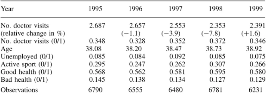
Table I gives summary statistics for the variables involved in the analysis. The average number of doctor visits per quarter declined from 2.66 to 2.35 between 1996 and 1998. This is more than an 11% reduction in the number of quarterly visits. There was a 1% decline between 1995 and 1996, and a 2% increase between 1998 and 1999. Thus, the large drop in the number of visits clearly coincides with the timing of the reform. Also, the 1999 ‘counter’ reform went hand in hand with an increased number of visits, again consistent with the hypothesis of a behavioural effect.
Throughout the sample period, there is a large fraction of non-users. The proportion is highest in 1998, when it reaches 37% of the sample, a 4.4 percentage point increase over the pre-reform year 1996. A simple Poisson distribution with parameter equal to the sample mean would predict a much lower proportion of non-users, e.g., 9.5% in 1998. Although this comparison does not take into account the variation generated by the regressors, it suggests the presence of extra zeros in the data.
The average age increased by less than a year between 1995 and 1999. This is a reflection of
the fact that the panel is not balanced. One reason for this is that young people enter the sample and old people leave since the sample is restricted to those aged 20–60 at any point in time, in addition to attrition and non-response. The unemployment to population ratio captures the state of
the business cycle. Indeed, it closely traces the movement of the official unemployment rate (see,
Table I. Sample means of doctor visits and selected socio-demographic character-istics, 1995–1999
Year 1995 1996 1997 1998 1999 No. doctor visits 2.687 2.657 2.553 2.353 2.391 (relative change in %) (1.1) (3.9) (7.8) (C1.6) No. doctor visits (0/1) 0.348 0.328 0.352 0.372 0.346 Age 38.08 38.20 38.47 38.73 38.92 Unemployed (0/1) 0.085 0.084 0.092 0.085 0.075 Active sport (0/1) 0.295 0.247 0.262 0.307 0.266 Good health (0/1) 0.568 0.562 0.581 0.595 0.580 Bad health (0/1) 0.145 0.138 0.134 0.127 0.129 Observations 6790 6555 6480 6781 6231
Source:German Socio-Economic Panel (GSOEP,ND32,837).
Finally, Table I also informs about the other health-related variables used in the analysis. Interestingly, the statistics indicate a general improvement in the health status of the population between 1996 and 1998. The proportion of people in active sports increased from 25 to 31%, although these averages are very volatile. A steadier trend is observed for the self-reported health condition. The proportion of people reporting good health increased from 56 to 60%, while the proportion of people reporting poor health decreased from 14 to 13%. These trends are important for two reasons. Firstly, improvements in the perceived health might be able to explain part of the reduction in the number of doctor visits, and one should control for that in order to isolate the reform effect. Secondly, these improvements provide some evidence against the possibility that the reforms, while being successful in containing costs, actually worsened the general health status. Of course, these self-reports are only a very crude measure of health, and more research would be needed to study the long-term consequences of expenditure reductions in the health sector on public health. This is beyond the scope of the current analysis.
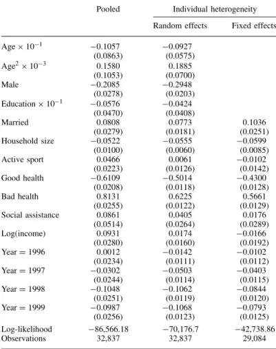
The estimates for the basic Poisson model, with and without individual specific effects, are
displayed in Table II. The first column shows the estimates from a pooled Poisson model. The
robust standard errors account for unobserved heterogeneity and correlation across time. The
second column displays the result from a Poisson model with gamma distributed individual specific
random effects (i.e., a panel negative binomial model). The fixed effects Poisson estimates are
given in the third column. In this model, all time-invariant regressors have to be dropped, as well as all observations pertaining to individuals without variation in the dependent count. Most
effects are robust to the particular model specification, and many of the results are common to
those found elsewhere in the literature: men have less doctor visits than women, and the expected number of doctor visits is u-shaped in age. The health indicators have the largest effect among all variables, although the effect is somewhat attenuated in the panel models. Most importantly the coefficients on the year dummies indicate that there was a statistically significant decline in the
expected number of doctor visits between 1996 and 1998 in all three model specifications. Based
on the pooled Poisson model, the expected number of visits fell by 9.9%.
Six additional models were estimated using the same data: negative binomial,
Poisson-log-normal, hurdle-negative binomial, finite mixture negative binomial with two components,
multi-episode model, and the probit-Poisson-log-normal model. The following discussion of the models is guided by the following questions: Is the result found in the base Poisson model robust with respect to model choice? Can the Deb and Trivedi (2002) conclusion of the superiority of the
Table II. Poisson results
Pooled Individual heterogeneity Random effects Fixed effects Ageð101 0.1057 0.0927 (0.0863) (0.0575) Age2ð103 0.1580 0.1885 (0.1053) (0.0700) Male 0.2085 0.2948 (0.0278) (0.0203) Educationð101 0.0576 0.0424 (0.0470) (0.0408) Married 0.0808 0.0773 0.1036 (0.0279) (0.0181) (0.0251) Household size 0.0522 0.0555 0.0599 (0.0100) (0.0060) (0.0085) Active sport 0.0466 0.0061 0.0102 (0.0223) (0.0126) (0.0142) Good health 0.6109 0.5014 0.4300 (0.0208) (0.0118) (0.0128) Bad health 0.8131 0.6225 0.5661 (0.0255) (0.0122) (0.0129) Social assistance 0.0861 0.0405 0.0176 (0.0514) (0.0264) (0.0289) Log(income) 0.0931 0.0174 0.0166 (0.0280) (0.0160) (0.0192) YearD1996 0.0012 0.0142 0.0102 (0.0234) (0.0111) (0.0112) YearD1997 0.0302 0.0503 0.0403 (0.0244) (0.0114) (0.0115) YearD1998 0.1048 0.1062 0.0844 (0.0251) (0.0119) (0.0120) YearD1999 0.0987 0.1068 0.0793 (0.0256) (0.0123) (0.0125) Log-likelihood 86,566.18 70,176.7 42,738.86 Observations 32,837 32,837 29,084
Source: GSOEP, own calculations. Model in addition includes three quarterly dummies and indicators of employment status. Standard errors in parentheses (pooled model with robust standard errors to account for unobserved heterogene-ity and serial correlation). The random effects model assumes gamma distributed individual effects.
finite mixture model over the hurdle model be confirmed? And to what extent can one uncover
asymmetries in the responses to the reform in different parts of the distribution (i.e., attribute the mean effect to different sources)?
There are several ways to discriminate between the models. Some of the models are nested
(such as the Poisson and the negative binomial model), most of them are not (such as the finite
mixture, the hurdle negative binomial and the multi-episodes models). Table III shows the log-likelihood values of the different models. Likelihood ratio tests clearly reject the Poisson model against the alternative models with unobserved heterogeneity. To pick the best model among all
seven, a comparison of the simple likelihoods is a first indicator. One can compute for instance
Table III. Model selection
Log-likelihood Parameter SICa Sb Poisson 86,566.18 22 173,361.14 7.16 Unobserved heterogeneity:
Negative binomial 64,611.55 23 129,462.28 13.97 Poisson-log-normal 64,202.78 23 128,644.74 14.15 Hurdle models:
Hurdle negative binomialc 64,252.16 46 128,982.68 14.13 Probit-Poisson-log-normal 63,871.90 45 128,211.78 14.30 Finite mixture model:
Two-components negative binomial 64,020.05 47 128,528.87 14.23 Multi-episode model:
Poisson-logarithmic 64,246.58 44 128,950.73 14.13 aSICD 2 lnLCKlnN.
bSDexplnL/Nð100.
cBoth hurdle and positive part are specified using the type 2 negative binomial probability function.
However, both the log-likelihood and theSstatistics do not account for the fact that the number
of parameters differ across the estimated models. Hence, the Schwartz Information Criterion (SIC) is included as well. The selection result stays the same regardless of what criterion is chosen. The new model with probit hurdle and log-normal unobserved heterogeneity offers a substantial improvement over all other models. One should also point out that the results corroborate the
Deb and Trivedi (2002) conclusion that the finite mixture negative binomial model outperforms
the hurdle negative binomial model. Thus their result can be interpreted as evidence against the particular hurdle parameterization, but not against hurdle models in general.
To analyse the particular relationship between the two hurdle models, thefinite mixture model
and the multi-episode model more formally, one can use Vuong’s (1989) test for model selection among non-nested models. This test does not require either of the two models to be correctly specified, but rather picks the model that is closer to the true distribution. The test is directional and symmetric. Under the null hypothesis that the two models are equivalent, the test statistic
N iD1 logfyijxiloggyijxi N iD1 logfyijxiloggyijxi2
is standard normally distributed. Note that the numerator is nothing else than the log of the likelihood ratio. In the present setting, one needs to realize that the models are, in the terminology of Vuong (1989), overlapping rather than strictly non-nested. For example, the probit-Poisson-log-normal model and the hurdle negative binomial can both be reduced to a simple Poisson model under appropriate parameter restrictions. Following Vuong (1989), therefore, a pre-test is generally required before the usual statistic can be computed. However, in practice it is sufficient to establish that the condition for overlap can be rejected in each model (see Vuong, 1989, footnote 6), which is the case in all of the models.
To implement the test, one chooses a critical valuec from the standard normal distribution. If
the alternative that model f is better than model g. If the test statistic is smaller than c,g is
better thanf. The test statistic for the probit-Poisson-log-normal against thefinite mixture model
is 5.7, against the hurdle negative binomial model 13.7, and against the multi-episode model 12.1. Hence, the null hypothesis is rejected in all three cases in favour of the new model. A comparison offinite mixture and hurdle models has a test statistic of 5.7.
Table IV reports the parameter estimates for the probit-Poisson-log-normal model. The first
column gives the coefficients for the hurdle part, the second for the positive part. Due to the
parameterization of the model (the hurdle is parameterized for the event of no visit), the coefficients should normally be of opposite sign, implying that the effect of a variable on the probability of use and on the extent of use, given use, go in the same direction. The sign and magnitude of
the effects is determined by the data and not imposed a priori. The ‘sign test’ indeed shows
only one deviation, in the case of the variable ‘education’. For the variable ‘active sport’, the
Table IV. Probit-Poisson-log-normal model
Probit0/1C Truncated Poisson-log-normal1C
Ageð101 0.2734 0.1100 (0.0559) (0.0557) Age2ð103 0.3538 0.1458 (0.0688) (0.0675) Male 0.4027 0.1228 (0.0170) (0.0166) Educationð101 0.1609 0.1406 (0.0330) (0.0342) Married 0.1394 0.0555 (0.0188) (0.0185) Household size 0.0344 0.0404 (0.0061) (0.0061) Active sport 0.1429 0.0094 (0.0173) (0.0174) Good health 0.4586 0.4750 (0.0174) (0.0176) Bad health 0.5720 0.6652 (0.0288) (0.0195) Social assistance 0.0457 0.1279 (0.0413) (0.0413) Log(income) 0.1293 0.0351 (0.0203) (0.0195) YearD1996 0.0671 0.0098 (0.0233) (0.0231) YearD1997 0.0017 0.0191 (0.0233) (0.0228) YearD1998 0.0595 0.0450 (0.0230) (0.0237) YearD1999 0.0092 0.0746 (0.0236) (0.0229) 2 0.8015 (0.0066) Log-likelihood 19,524.36 44,347.54 Observations 32,837 21,365
Note: Model in addition includes three quarterly dummies and indicators of employment status. Standard errors in parentheses.
impact on the probability of non-use is statistically significant but the impact on the positives is insignificant.
The size and composition of the reform effect, measured by the percentage reduction in the expected number of doctor visits, for each of the models under consideration is listed in Table V. The estimates for the base model, with or without unobserved heterogeneity, are all in the same range, varying between 9.9 and 10.4%. These estimates are substantially above those of
the Lauterbach et al. study, which reported a decline of 4.5%. How can these two findings be
reconciled? It is possible that the differences have to do with the low response rate in their survey, or the way the question was posed that differs from the GSOEP approach. The analysis of this paper suggests, however, a more fundamental reason, namely the fact that the Cologne study sampled individuals on-site and thus overrepresented heavy users. If it is the case that heavy users
have a lower demand elasticity than occasional users, the two findings can be reconciled.
The structural models estimated above can exactly deal with this question of different elasticities
in different parts of the distribution. Table V confirms that such a differential effect is present
indeed. This is most obvious from the probit-Poisson-log-normal estimates. The reduction is greatest at the left margin of the distribution: the probability of being a user (at least one visit) decreased by an estimated 6.7% between 1996 and 1998, whereas the expected number of visits, conditional on use, decreased only by an estimated 2.6%. Compare this to the alternative of a
single Poisson-log-normal model without hurdle. In this case, the implied changes are 3.0%
for PY >0and 6.1% for EYjY >0, respectively. Hence, the evidence clearly suggests an excess sensitivity at the left tail of the distribution.
This important result is confirmed by the other two structural models, although quantitative
details differ. The finite mixture model separates the population into two groups. Two-thirds of
the population belong to a low-user group with a mean number of quarterly visits of 1.6, and one-third belongs to a high-user group with a mean number of 3 visits per quarter. Consistent with the above argument, the low-user group shows a larger response to the reform, with a 13% reduction. Similarly, in the multi-episode model, the effect on the number of spells is much greater than the effect on the number of referrals (which actually are estimated to have slightly increased
Table V. Evaluation of the reform effect
% (96,98) Poisson model 9.9 Negative binomial 8.9 Poisson-log-normal 10.4 Two-components negative binomial
Group 1 (p1D0.663, 1D1.59) 12.9 Group 2 (p2D0.337, 2D3.01) 4.9 Total 10.2 Probit-Poisson-log-normal HurdlePY >0 6.7 Positives EYjY >0 2.6 Total 9.1 Poisson-logarithmic (multi-episodes) Spells 10.2 Referrals C1.3 Total 9.1
by 1.3%). In each case, the two effects add up to a combined effect in the neighbourhood of a 10% reduction in the number of visits between 1996 and 1998.
7. DISCUSSION
The analysis showed that the German health care reform of 1997 affected the left tail much more than the positive part of the distribution of the number of doctor visits. To the extent that the positive part represents the subpopulation of the seriously or chronically ill, whereas the left end of the distribution represents the healthy, this might have been an intended consequence of the reforms.
How reasonable is it to interpret the uncovered reform effects as causal? Identification is
achieved by studying variation in the demand for doctor visits over time. Thus, it is assumed that other things did not change concurrently, beyond the individual socioeconomic characteristics controlled for in the regression. It is hard to imagine what these other things should have been. It is unlikely that the underlying unobserved health status varied substantially between the two years beyond the controls, or that a health epidemic of major proportion hit in 1996 but was absent in 1998.
A further potential confounder is the business cycle. In times of high unemployment, employed people may reduce their demand for doctor visits to a minimum, in order to reduce the risk of being perceived as a shirker. However, West German unemployment rates were very similar in the two years (9.1% in 1996 versus 9.2% in 1998), making this an implausible explanation as well.
Certainly, future work needs to pursue these issues further. Such work can build on the methodological insights of this paper. When studying the effects of reforms on the demand for doctor visits, hurdle or two-part models should be given serious consideration. Of course, these models are only one possible way to generalize the rigid assumptions underlying single index models such as the standard Poisson or negative binomial regressions. A very promising alternative, quantile regression models for count data, is currently being developed by Machado and Santos Silva (2002).
APPENDIX: THE DATA SET
The data are extracted from the German Socio-Economic Panel, 1995–1999. I use observations on men and women aged 20–60 from Sample A, i.e., persons associated with non-guestworker households in the original sample for West Germany. Privately insured individuals (about 6% of the sample) are excluded from the analysis. Accounting for observations with missing values on
any of the dependent or independent variables, thefinal sample comprises 32,837 observations.
Definition of Variables
Doctor consultations is the self-reported number of visits to a doctor during the three months prior to the interview.
Male is an indicator variable taking the value of one if the individual is male.
Married is an indicator variable taking the value of one if the individual is married. Household size is the number of persons living in the household.
Active sport is an indicator variable taking the value of one if the individual participates in sports at least once a week.
Good health is an indicator variable taking the value of one if the individual classifies his/her own health as either ‘very good’ or ‘good’.
Bad health is an indicator variable taking the value of one if the individual classifies his/her own health as either ‘very bad’ or ‘bad’ (‘fair’ is the omitted reference category).
Full-time employed is an indicator variable taking the value of one if the individual is in full-time employment at the time of the interview.
Part-time employed is an indicator variable taking the value of one if the individual is in part-time employment at the time of the interview.
Unemployed is an indicator variable taking the value of one if the individual is unemployed at the time of the interview.
Log(income) is the logarithmic household equivalent income, where the OECD scale has been
applied (weight of 1 for the first person, 0.7 for the second person, and 0.5 for each
additional person). Income is expressed in 1995 values using the CPI deflator published by
Sachverst¨andigenrat (2000).
ACKNOWLEDGEMENTS
I am grateful to Maarten Lindeboom, Joao Santos Silva, seminar participants at IZA, the universities of Heidelberg, M¨unchen, G¨ottingen, Z¨urich, Dortmund, Kiel, Tinbergen Institute, the IZA-CEPR European Summer Symposium in Labor Economics 2001, and two anonymous referees for helpful comments.
REFERENCES
Breyer F, Zweifel P. 1999.Gesundheits¨okonomie. Springer: Heidelberg.
Deb P, Trivedi PK. 2002. The structure of demand for health care: latent class versus two-part models. Journal of Health Economics 21: 601–625.
Grossman M. 1972. On the concept of health capital and the demand for health.Journal of Political Economy
80: 223–255.
Lauterbach KW, Gandjour A, Schnell G. 2000. Zuzahlungen bei Arzneimitteln. Powerpoint presentation at http://www.medizin.uni-koeln.de/kai/igmg/stellungnahme/zuzahlungen/index.htm, version 25.2.2000. Machado JAF, Santos Silva JMC. 2002. Quantiles for counts. Institute for Fiscal Studies, University College,
London, Cemmap Working Paper CWP22/02.
Mullahy J. 1986. Specification and testing in some modified count data models.Journal of Econometrics33: 341–365.
Sachverst¨andigenrat. 2000.Chancen auf einen h¨oheren Wachstumspfad, Jahresgutachten 2000/01. Metzler-Poeschel: Stuttgart.
Santos Silva JMC. 1997. Unobservables in count data models for on-site samples. Economics Letters 54: 217–220.
Santos Silva JMC, Windmeijer F. 2001. Two-part multiple spell models for health care demand.Journal of Econometrics 104: 67–89.
Smith MD, Moffatt PG. 1999. Fisher’s information on the correlation coefficient in bivariate logistic models. Australian and New Zealand Journal of Statistics 41: 315–330.
SOEP Group. 2001. The German Socio-Economic Panel (GSOEP) after more than 15 years—overview. In Proceedings of the 2000 Fourth International Conference of German Socio-Economic Panel Study Users (GSOEP2000), Holst E, Lillard DR, DiPrete TA (eds).Vierteljahrshefte zur Wirtschaftsforschung70: 7–14. Vuong QH. 1989. Likelihood ratio tests for model selection and non-nested hypotheses.Econometrica 57:
307–333.