Testing Linearity in Cointegrating Relations with an Application to Purchasing Power Parity

TESTING LINEARITY IN COINTEGRATING RELATIONS

WITH AN APPLICATION TO PURCHASING POWER PARITY

By

Seung Hyun Hong and Peter C. B. Phillips

December 2005

COWLES FOUNDATION DISCUSSION PAPER NO. 1541

COWLES FOUNDATION FOR RESEARCH IN ECONOMICS

YALE UNIVERSITY

Box 208281

Testing Linearity in Cointegrating Relations with an Application

to Purchasing Power Parity

Seung Hyun Hong∗ Department of Economics

Concordia University

and

Peter C. B. Phillips†

Cowles Foundation, Yale University University of Auckland and University of York

November 13, 2005

Abstract

This paper develops a linearity test that can be applied to cointegrating relations. We consider the widely used RESET specification test and show that when this test is applied to nonstationary time series its asymptotic distribution involves a mixture of noncentralχ2

distributions, which leads to severe size distortions in conventional testing based on the cen-tralχ2_{. Nonstationarity is shown to introduce two bias terms in the limit distribution, which}

are the source of the size distortion in testing. Appropriate corrections for this asymptotic bias leads to a modified version of the RESET test which has a centralχ2 _{limit distribution}

under linearity. The modified test has power not only against nonlinear cointegration but also against the absence of cointegration. Simulation results reveal that the modified test has good size in finite samples and reasonable power against many nonlinear models as well as models with no cointegration, confirming the analytic results. In an empirical illustra-tion, the linear purchasing power parity (PPP) specification is tested using US, Japan, and Canada monthly data after Bretton Woods. While commonly used ADF and PP cointegra-tion tests give mixed results on the presence of linear cointegracointegra-tion in the series, the modified test rejects the null of linear PPP cointegration.

JEL Classification: C12, C22

Key words and phrases: nonlinear cointegration, specification test, RESET test, noncentral

χ2 distribution

∗_{Department of Economics, Concordia University, 1455 de Maisonneuve Blvd. West, Montreal, Quebec H3G}

1M8, Canada; e-mail: [email protected]

†_{Cowles Foundation for Research in Economics, Yale University, Box 208281, New Haven, CT 06520-8281,}

1

Introduction

Economic time series are often believed to exhibit nonlinear behavior and economists usually formulate this nonlinearity in one of the following two ways: (i) by building nonlinear dynamics into the model for an individual time series; or (ii) by allowing for nonlinearity in the relationship between time series. This paper investigates issues associated with the second approach and does so from a model specification perspective. Since the introduction of the cointegration concept, linear models have dominated practical work in cointegration analysis. This emphasis has arisen, not so much because the underlying economic theory suggests linearity, but rather because the cointegration concept and associated econometric methodology has been developed very largely for linear models of integrated processes. Correspondingly, the tools of econometric analysis are available in this case and there is great convenience in computation for applied work. In contrast, until recently, there has been a lack of appropriate analytic tools for considering nonlinearly transformed integrated time series and an absence of an asymptotic theory of inference.

Empirical applications often stimulate an interest in nonlinear specifications and, in conse-quence, many nonlinear models (and almost as many specification tests) have been developed for stationary time series modeling. Many recent nonlinear model applications of nonstationary time series have focused on nonlinear short-run dynamics around linear long-run equilibria in error correction models (ECM), as in Berben & Dijk (1999), Lo & Zivot (2001), and Ter¨asvirta & Eliasson (2001) among others. Few attempts have been made to study nonlinear cointegrating relations directly and the methods that have been tried in practical work often require restrictive conditions on the DGP (e.g. Basher & Haug, 2003). Such extensions also await a corresponding development in tests of specification.

Neglecting the possibility of nonlinearity in a long-run relationship can be particularly detri-mental in nonstationary cases. For stationary time series, linear models can often provide workable approximations at least locally to nonlinear models. Unlike mean-reverting stationary processes, nonstationary time series have a tendency to wander with no fixed mean or locality in the sample space and, like random walks, revisit points distant from the origin an infinite number of times. In such cases, local linear approximations can only poorly represent the global characteristics of the process, producing a high risk of faulty inference about a misspecified long-run equilibrium.

Considerations of the possibilities suggest three cases – linear cointegration, some form of nonlinear cointegration, or complete absence of cointegration. Existing cointegration tests essen-tially presume a form of linear cointegration and do not effectively distinguish between linear and nonlinear cointegration (Granger & Hallman, 1989). So, linear cointegration analysis requires an additional test of specification to address this particular issue. Existing linearity tests also fail to provide any guidance concerning the type of relationship that may be present between nonstationary time series if it were nonlinear (Granger, 1995). Accordingly, it is not surprising to find that linearity tests which have been developed for stationary processes work poorly with nonstationary time series. This was well recognized earlier in the case of the RESET test.

The RESET test (Ramsey, 1969) is a convenient device for testing general misspecification (e.g. Vitaliano, 1987; Baghestani, 1991; Peters, 2000, among others), but is known not to be ro-bust to autocorrelated disturbances, especially when the regressor is itself highly autocorrelated (Porter & Kashyap, 1984) or contains a deterministic time trend (Leung & Yu, 2001). Using simulation experiments, Porter & Kashyap (1984) show that the presence of serially correlated

disturbances combined with an AR(1) regressor leads to size distortions, and the more autocor-related is the regressor the less robust the RESET test is to error autocorrelation. Naturally, we might expect this size distortion problem to become worse in the cointegrating case where the regressor has an autoregressive unit root and the errors are typically serially dependent.

In the absence of more appropriate specification tests, applied economists have treated ex-isting cointegration tests as tests for linear cointegration. In other words, if evidence for coin-tegration is found, it is conventionally assumed without further testing that such coincoin-tegration is linear in nature and all subsequent analysis rests on this assumption. The present paper develops a direct testing method that can answer the simple but important question: do the data support a linear cointegrating specification? To do so, we modify the widely used regres-sion error specification test (RESET), which is a linearity test based on general approximation theory. The RESET test implicitly uses a Taylor series approximation to capture unspecified nonlinear forms by seeking to detect nonlinearities that remain in the linear regression residuals using a linear combination of polynomial functions. Our approach here is to use recently devel-oped asymptotic tools for nonlinearly transformed integrated time series from Park & Phillips (1999, 2001) to modify the RESET test in an appropriate manner so that it can be applied to nonstationary time series to test directly for linearity in cointegrating relations.

The rest of this paper is organized as follows. The next section introduces the model and the maintained assumptions and shows how the testing method is related to an underlying theory of nonlinear approximation. In addition, we show how the nonstationarity of the data changes the limiting theory of the existing test using sample covariance asymptotics of nonlinearly trans-formed integrated processes. Section 3 discusses the modifications that are needed when the RESET test is applied to cointegrating relations. The asymptotic distribution of the modified test statistic is discussed both for the null and various alternative hypotheses. Simulation results on the finite sample size and the power of the modified test are reported in Section 4. Section 5 presents an empirical application of the modified test to purchasing power parity (PPP). Sec-tion 6 concludes and addiSec-tional assumpSec-tions, lemmas and proofs are collected together in the Appendix.

2

Model and Background Ideas

The RESET test utilizes an approximate representation based on a power series expansion to determine whether the linear specification leaves anything unexplained in the regression residuals that can be detected by a linear combination of polynomial basis functions. The idea can be naturally extended to other families of basis functions and, as we will show, utilized in the context of nonstationary data applications.

For an arbitrary functionf(x) lying in a suitably defined L2 function space over a certain

domain, it is possible to construct an orthogonal series representation of the following form

f(x)≈ ∞ X j=1 β_jF_j(x) or in two parts f(x) ≈ k X j=1 β_jF_j(x) + ∞ X j=k+1 β_jF_j(x) = ˆf_k(x) +error

in terms of some basis functions {Fj(x)} that form a complete set and where ≈ signifies L2

use simple polynomials as a basis. Given f(x), the accuracy of the finite sum approximation ˆ

fk(x) =

P_k

j=1βjFj(x) or the size of the “error” term depends on the number of terms (k)

included in the sum and the properties of the function f, on which there is a huge literature in Fourier series analysis (e.g. Tolstov, 1976).

Suppose that we want to test the linear conditional mean specificationH0 :P[E(Yt|Xt) =

θ1Xt] = 1, ∀t using a regression specification

Yt=θ1Xt+θ2f(Xt) +ut. (1)

If one has a specific nonlinear alternative model in mind, such as (1) for some given f(X_t), and wants to test that specific model against the linear model, then one can use tests such as a Wald or LM test of H0 :θ2 = 0 to decide which model fits the data better. In many practical

cases, however, theory fails to provide a specific functional form, and while it is possible to come up with alternate nonlinear models, these often seem rather arbitrary. Also, if the focus of attention is some convenient linear model (such as that implied by purchasing power parity considerations) with no specific nonlinear alternative, then it is of particular interest to test whether the linear specification is “acceptable”. A linearity test based on approximation theory seems appropriate in these situations.

Replacing the unspecified nonlinear functionf(X_t) with a partial sum approximation ˆf_k(X_t), we may proceed to test the validity of the linear specification by testing whether a linear combi-nation of a finite number of suitable basis functions {Fj(·)}k1 can detect any nonlinearity in the

regression residuals. This procedure involves testingH₀ :β_j = 0, ∀j in the regression

Yt=θXt+ut and ˆut= k

X

j=1

β_jFj(Xt) +et, (2)

where the ˆu_tare the regression residuals and the basis functions are chosen to beF_j(X_t) =X_tj+1

for the RESET test1. As is apparent, using this approach there can be as many tests of linearity as there are approximation methods2_{. Here we will focus on the RESET test in view of its}

popularity in applied work.

Note that estimation of (2) involves working with the sample moments of nonlinearly trans-formed integrated time series of the form P_tFj(Xt)ˆut and

P

tFj(Xt)Fi(Xt),whose asymptotic

behavior must be characterized. Before examining these quantities, we first specify the data generating processes and some assumptions that will facilitate the development of a limit the-ory.

Assumption A: Let 4Xt = vt and ut be general linear processes satisfying the following

1_{While the original test by Ramsey (1969) and the similar tests by Keenan (1985) and Tsay (1986) use the}

fitted value ˆYt, Thursby & Schmidt (1977) propose using the polynomials ofXt instead for a higher power.

2_{For example, DeBenedictis & Giles (1998) use a Fourier series approximation idea that has better global}

fitting capability than a Taylor series approximation, while Keenan (1985), Tsay (1986) and Barahona & Poon (1996) use variations of Volterra series expansions. White (1989) presents a neural network (NN) test based on the cdf of the logistic distribution and Blake & Kapetanios (2000) develop another NN test using radial basis functions for artificial neural networks.

conditions. ut = ∞ X j=0 cjεt−j =C(L)εt vt= ∞ X j=0 djηt−j =D(L)ηt ˜ ζ_t = µ η_t+1 εt ¶

is a stationary and ergodic martingale difference sequence with natural filtration F_t=σ

³

{˜ζ_s}t_−∞

´

and variance matrix Σ = µ

σ11 σ12

σ21 σ22

¶

and where {cj, dj} satisfy the conditions

D(1)6= 0, ∞ X j=0 j|dj|<∞, and ∞ X j=0 j1/2|cj|<∞

These assumptions on the innovation processes are fairly standard, although in some cases below the linear processXtis assumed to be predetermined in the sense thatE(Fj(Xt)|Ft−1) =

Fj(Xt). Conditions similar to these assumptions and Assumption A1 in the Appendix (an

additional technical moment condition) are employed in deriving the results of Park & Phillips (1999, 2000, 2001) and Chang, Park & Phillips (2001). However, De Jong’s (2002) more relaxed conditions are sufficient for the modification of the RESET test presented in this paper.

Under Assumptions A and A1, the following invariance principle holds 1 √ n [nr] X t=1 ˜ ζ_t⇒dW(r)≡ µ W1(r) W2(r) ¶ ≡BM(Σ),

and using the Beveridge-Nelson decomposition (Phillips & Solo (1992)), we can show that a similar result holds for the time series ζ_t= [vt, ut]0.

1 √ n [nr] X t=1 ζ_t⇒dB(r)≡ µ Bx(r) Bu(r) ¶ ≡BM(Ω).

Here the covariance matrix Ω = P∞_h=−∞Γ_ζ(h), where Γ_ζ(h) = E(ζ₀ζ0

h). It is convenient to

partition Ω conformably with ζ_t as

Ω = µ Ωvv Ωvu Ωuv Ωuu ¶ , (3)

and to define and partition the one-sided long-run covariance matrix

Λ = ∞ X h=1 Γζ(h) = µ Λvv Λvu Λuv Λuu ¶ , (4) 4 = Γ_ζ(0) + Λ = µ ∆vv ∆vu ∆uv ∆uu ¶ . (5)

Among the wide variety of possible nonlinear functions, Park & Phillips (1999, 2001) pro-vide asymptotic tools for certain classes of functions (of integrated processes) satisfying some regularity conditions. The simple basis functions {X_tj} of a Taylor series expansion fall within the H-regular (or Class H) class, which is defined as follows.

Definition 1 A transformationF(·) is said to be H-regular iff

F(λx) =κ(λ)H(x) +R(x, λ) where H(·) is locally integrable, and R(·,·) is such that

• |R(x, λ)| ≤ a(λ)P(x), where lim sup_λ→∞a(λ)/κ(λ) = 0 and P(·) is locally integrable, or

• |R(x, λ)| ≤b(λ)Q(λx), where lim sup_λ→∞b(λ)/κ(λ)<∞ and Q(·) is locally integrable and vanishes at infinity, i.e. Q(x)→0 as |x| → ∞

Functions in this class have homogenous, asymptotically dominating componentsκ(λ)H(x) that are locally integrable. H(x) is referred as theasymptotic homogenous function of F(x) and

κ(λ) as the asymptotic order of F(x). Park & Phillips (1999) provide various examples that belong to this class, such as finite order polynomials, logarithmic functions, and distribution-like functions, including their linear combinations and products. The basis functions{Fm=Xm+1}

from a Taylor series expansion belong to this class with H(x) =xm+1 _{andκ(λ) =λ}m+1_.

Another important class of nonlinear transformation is the I-regular (or Class I) transforma-tion. Roughly speaking, functions in this class are bounded, integrable and (piecewise) smooth (see Park & Phillips (1999) for further details). All pdf-like functions belong to this class.

2.1 A Linearity Test and Sample Covariances of Nonlinearly Transformed Xt

As a first step in the development, consider the simplest case where Xt is strictly exogenous

so that Assumption A holds with E(vtus) = 0 for all t, s and the long-run covariances Ωuv =

Λuv= 0. Both OLS and FM-OLS (Phillips and Hansen, 1990) estimators ofθ in (2) then yield

consistent and asymptotically mixed normally distributed ˆθ, and the RESET test statistic for

H0 :βj = 0,∀j follows a limiting centralχ2(k) distribution, as we now show. That is

Rn= à _n X t=1 ˆ utFt !₀à ˆ Ωuu.v n X t=1 ˜ FtF˜t0 !₋₁à _n X t=1 ˆ utFt ! A ∼ χ2(k), (6) with ˜ Ft=Ft−Xt à X t FtFt0 !₋₁ X t XtFt for Ft= h X_t2 · · · X_tk+1 i₀ , (7)

and where ˆΩuu.v is a consistent estimator of Ωuu under exogeneity. The test statistic Rn is a

quadratic form of sample covariances between a nonlinearly transformed integrated process and the fitted residuals, viz.,

n X t=1 µ Xt √ n ¶_m ˆ ut √ n = n X t=1 ^ µ Xt √ n ¶_m ut √ n ⇒ d Z g Bm x dBu, (8)

where the tilde over a variable implies that it is the residual from a linear regression of that variable on Xt for a finite sample, and equivalently for the limit processes where we write the

projection residuals asBgm x =Bxm−Bx( R B2 x)−1 R Bm+1 x ,where R

with respect to Lebesgue measure. The latter notation is used throughout the paper. The limit (8), conditional onFx =σ(Bx(r),0≤r ≤1), is a mean-zero Gaussian mixture

Z g Bm x dBu ¯ ¯ ¯ ¯ Fx ∼ N µ 0,Ω_uu Z g Bm x 2¶ ,

so that, combined with the limit of the sample variance

1 n n X t=1 ^ µ Xt √ n ¶_mµ_^ Xt √ n ¶_m ⇒ Z g Bm x 2 ,

and a consistent estimator for Ωuu, the RESET test statistic (6) has the following limit

Rn⇒d µZ g Bm x dBu ¶₀µ Ωuu Z g Bm x 2¶−1µZ _g Bm x dBu ¶¯¯ ¯ ¯ ¯ Fx ∼χ2(k)

conditional onFx. Since the limit distribution is independent ofFx, we deduce thatRn⇒χ2(k)

unconditionally.

Next, we discard the “strong exogeneity” condition onXt so that Assumption A holds with

Ωuv 6= 0. Abandoning the strong exogeneity condition changes the previous result in several

ways. First, the least squares estimator ofθ now has two second order bias terms in the limit, viz., n ³ ˆ θ−θ ´ = Ã 1 n2 n X t=1 X_t2 !₋₁ 1 n n X t=1 X_tu_t ⇒d µZ B_x2 ¶₋₁½Z BxdBu.x+ ΩuvΩ−vv1 Z BxdBx+4uv ¾ , (9)

where the Brownian motion B_u.x = B_u−Ω_uvΩ−1

vvBx is independent of Bx and has variance

Ωuu.v = Ωuu−ΩuvΩ−vv1Ωvu.In (9) the term

R

BxdBu.x is amean zero Gaussian mixture, but the

other two terms in braces shift the mean of the limit distribution away from zero. These terms correspond to the so-called endogeneity bias and serial correlation bias of linear cointegration theory (Phillips & Hansen, 1990), and stem from the nonstationarity of Xt. Similar effects

also generally arise with the sample covariance of ut with nonlinear transformations of Xt.

The following lemma summarizes the effects when the sample covariances involve polynomial functions.

Lemma 2 Under Assumptions A and A1, the sample covariance betweenXm

t and ut satisfies 1 n(m+1)/2 n X t=1 X_tmut⇒d Z B_xmdBu.x+ ΩuvΩ−vv1 Z B_xmdBx+m∆vu Z B_xm−1 (10) with ∆vu = P_∞ h=0E(v0uh).

Lemma 2 shows that, as in the linear cointegration case (9), sample covariances of nonlinear functions and stationary processes have limits that also involve two bias terms that produce nonzero location effects in the limit distribution of {βˆ_j} in (2). We refer to these effects as “bias” terms because both terms shift the location of the limit distribution of ˆβ_j away from the true value β_j. The three components in the limit distribution in (10) are a mean-zero Gaussian mixture and two bias terms stemming from endogeneity and serial correlation effects, the latter being random when m >1.

De Jong (2002) examines this nonlinear sample covariance asymptotics under conditions that are less strict on the innovation processes, but more restrictive in terms of functional forms. He shows that for an H-regular functionF(·) withcontinuously differentiable asymptotic homogeneous functionH(·), the sample covariance ofF(Xt) withut satisfies

1 n1/2_κn n X t=1 F(Xt)ut ⇒d Z H(Bx)dBu+4uv Z H0(Bx) (11)

where the asymptotic order of H(·) is κn =κ(

√

n). With F(z) =zm_{, we haveH(z) =z}m _and

κ_n = nm/2_{, so that (11) then reduces to (10) in Lemma 2. A recent and much more general}

semimartingale approach to establishing limit results such as (11) is developed in Ibragimov and Phillips (2004).

The effects from the bias terms in Lemma 2 can be substantial in the RESET test statistic (6). As is well known (e.g., Muirhead, 1982, theorem 1.4.5), a necessary and sufficient condition for the quadratic formx0_{A xin the Gaussian random vectorx≡ N(ξ, V),whereV is nonsingular, to}

follow a noncentral χ2 _{distribution is thatAV be idempotent.In this event x}0_{A x is noncentral}

χ2(k, ν), where k = rank(AV) is the degrees of freedom and ν = ξ0A ξ is the noncentrality parameter. Here, we can replacexwith the limit ofPn_t=1uˆtFtafter an appropriate normalization

and suitable conditioning, and thereby show that the test statistic Rn in (6) follows a mixture

of noncentral χ2 distributions, giving the following asymptotic result for the test when the exogeneity condition onXt does not hold.

Theorem 3 Under Assumptions A and A1, the RESET test statisticRn has asymptotically a

mixture noncentralχ2 _{distribution withkdegree of freedom and random noncentrality parameter}

ν =ξ0A ξ. That is, Rn = Ã _n X t=1 ˆ utFt !₀Ã ˆ Ωuu.v n X t=1 ˜ FtF˜t0 !₋₁Ã _n X t=1 ˆ utFt ! = ˆu0F ³ ˆ Ω_uu.vF˜0F˜ ´₋₁ F0uˆ ∼A χ2(k, ν) for F˜t defined in (7), F = [F1,· · · , Fn]0, F˜ = h ˜ F1,· · ·,F˜n i₀

, and where Ωˆuu.v is a consistent

estimator of Ωuu.v. The random noncentrality vector ξ is k×1 with (m−1)th element defined

as ξ(m−1) = ΩuvΩ−vv1 Z B_xmdBx+m4vu Z B_xm−1−Λvu µZ B_x2 ¶₋₁Z B_xm+1,

and A is a k×k covariance matrix A=     Ωuu.v      R f_B2 x 2 · · · R fB2 xB]xk+1 .. . . .. ... R _] Bxk+1Bfx2 · · · R _] Bkx+1 2           −1 with Bgm x =Bxm−Bx( R B2 x)−1 R Bm+1 x . Remarks

1. In general, the mean and variance of a quadratic form x0_{A x with a noncentral χ}2_{(k, ν)}

are (e.g., Johnson & Kotz, 1978)

E(x0A x) =k+1 2ξ

0_{A ξ and var(x}0_{A x) = 2(k+ξ}0_{A ξ).}

So, conditional on Fx =σ(Bx(r),0≤r ≤1), the first two moments of Rn can be written

as k+ 1₂ν and 2(k+ν) respectively, and they are greater than the central χ2(k) coun-terpart. This implies a higher probability of Type I errors, which explains the large size distortions observed in the simulation work by Porter & Kashyap (1984). We can check this by approximating the noncentral χ2(k, ν) distribution by a multiple of a central χ2

distribution, aχ2_{(b), where the two constants are given by (see Johnson & Kotz, 1978)}

a= 1 + ν

k+ν ≥1 and b=k+ ν2

k+ 2ν ≥k.

Therefore, conditional onF_x, the probability of rejecting the linearity null hypothesis can be written approximately as P[Rn> χ2α]∼P ·µ 1 + ν k+ν ¶ χ2(b)> χ2_α ¸ ≥P · χ2 µ k+ ν 2 k+ 2ν ¶ > χ2_α ¸ ≥α,

which is always at least as great as the nominal sizeα.

2. Originally, Ramsey (1969) introduced the RESET test as anF-test, where the test statistic can be written as Fn= (ˆu 0_uˆ−ˆe0_eˆ)/k ˆ e0_{e/ˆ (n−K−k)} = ˆ u0_(I−M F) ˆu/k ˆ u0_M F ·u/ˆ (n−K−k) , (12)

where ˆu and ˆe are the vectors of regression residuals from (2), K is the column number of Xt, and the k×k projection matrix MF = I −MXF(F0MXF)−1F0MX with MX =

I−X(X0_X)−1_X0 _{andX= [X}0

1,· · ·, Xn0]0. The numerator in (12) is equal to theχ2 version

of the RESET test Rn in Theorem 3 multiplied by ˆΩuu.v/k.That is,

1 kuˆ 0_(I−M F) ˆu= ˆ Ωuu.v k uˆ 0_F³_Ωˆ uu.vF0MXF ´₋₁ F0uˆ ∼A Ωuu.v k ·χ 2_{(k, ν).}

The denominator of (12) also can be shown to converge to Ω_uu.v/(n−K −k) times a mixture of noncentralχ2 random variableχ2(n−K−k, ν0) with noncentrality parameter

ν0 _=E(ˆu0_M

Fuˆ|X). Therefore, conditional on Fx, the ratio of two normalized noncentral

χ2 _{random variables follows a doubly noncentralF-distribution, denoted asF(k, n−K−}

k;ν, ν0),and

Fn⇒F(k, n−K−k;ν, ν0) withν =ξ0A ξ and ν0 =ξ0(I−A)ξ, (13)

forξandAdefined in Theorem 3. Johnson & Kotz (1978) show that this doubly noncentral

F-distribution can be approximated by a centralF-distribution

F(k, n−K−k;ν, ν0)≈ µ 1 +ν/k 1 +ν0_/(n−K−k) ¶ F(df1, df2),

with two degrees of freedom defined by

df1 =

(k+ν)2

k+ 2ν and df2 =

(n−K−k+ν0₎2

n−K−k+ 2ν0 .

Using this approximation, the probability of rejecting the linearity null hypothesis can be written as P[F_n> F_α]∼P[F(df₁, df₂)> F_α/C] withC = µ 1 +ν/k 1 +ν0_/(n−K−k) ¶ ,

with random noncentrality parameters ν andν0_{. Note that as long asξ 6= 0,C ⇒1 +ν/k}

asn→ ∞ and the noncentrality can therefore produce a substantial size distortion in the test.

3

Bias Correction and a Modified RESET Test

The previous section shows that nonstationarity of Xt introduces two bias terms in the limit

distribution of the sample covariance between Xm

t and ˆut, so that the RESET statistic Rn is

a limiting mixture of noncentral χ2 distributions. These bias terms are the main source of the large size distortions in the test and we now present a method to remove them, leading to the modified RESET test whose limit distribution is central χ2_{. The correction method is similar}

to that used in FM regression (Phillips and Hansen, 1990). After identifying sample quantities that converge to the bias terms, nonparametric corrections are implemented in the test statistic to eliminate them. For the first step, the following lemma introduces sample quantities that have the same limits as the bias terms.

Lemma 4 Let Assumptions A and A1 hold. Form≥1,

ˆ 4vum_n n X t=1 µ Xt √ n ¶_m−1 ⇒dm4vu Z B_xm−1, (14) and n X t=1 µ Xt √ n ¶_m vt √ n−4ˆvv m n n X t=1 µ Xt √ n ¶_m−1 ⇒d Z Bm_xdBx, (15)

Remarks

1. Lemma 4 provides sample quantities that converge to the asymptotic bias terms shown in Lemma 2. In linear cointegration, the corresponding terms for the two biases in (9) are given by ˆ ΩuvΩˆ−vv1 à 1 n n X t=1 Xtvt−4ˆvv ! ⇒dΩuvΩ−vv1 Z BxdBx and 4ˆuv⇒p 4uv

Denoting these two components as E_n and S_n, respectively, the sample covariance now becomes a mean zero Gaussian mixture in a linear case

1 n n X t=1 Xtut−En−Sn⇒d Z BxdBu.x,

and FM estimation simply applies these corrections, giving

n ³ ˆ θF M −θ ´ = Ã 1 n2 n X t=1 X_t2 !₋₁( 1 n n X t=1 Xtut−En−Sn ) ⇒d µZ B_x2 ¶₋₁Z BxdBu.x ¯ ¯ ¯ ¯ ¯ Fx ∼ N Ã 0,Ωuu.v µZ B_x2 ¶₋₁! (16)

We will use the same idea here to correct the bias terms in the test statisticRn.

2. De Jong (2002) also recognizes the presence of two biases in nonlinear cointegrating re-gressions and gives the same expression as ours for the serial correlation bias correction in (11), but takes a different approach to correct the endogeneity bias. Noting that FM regression corrects the endogeneity bias by replacing RB_xdB_u with R B_xdB_u.x, De Jong suggests a direct correction to the regression errors by using u_t−Ωˆ_uvΩˆ−1

vvvtinstead ofut.

The sample quantities and their limits shown in Lemma 4 are closely related to the noncen-trality vector ξ defined in Theorem 3. Since the test statisticRn is a quadratic form involving

sample covariances of nonlinear functions, and the noncentrality parameter of its limit distri-bution correspondingly involves a quadratic form of ξ, we may eliminate the noncentrality by subtracting the sample quantities that converge toξfrom the nonlinear sample covariances. The following theorem explains how to accomplish this modification of the RESET test and remove the noncentrality.

Theorem 5 Suppose Assumptions A and A1 hold. If {Xt, Yt} are linearly cointegrated, the

following modified RESET statistic has a limiting central χ2 _{distribution with degrees of freedom}

k MRn= © ˆ u0F·Dn−En0 −Sn0 ª ³_ˆ Ωuu.vD0nF˜0F˜·Dn ´_−1© Dn·F0uˆ−En−Sn ª _A ∼ χ2(k),

where uˆ is n×1 vector of residuals from the linear cointegration regression (2), F is an n×k

matrix with the (m, t) element X_tm+1, andF˜ is the regression residual from regressingF on Xt

as in Theorem 3. The k×k normalization matrix Dn and the (m−1)th elements of the two

k×1 correction vectors E_n= [E_n(1),· · ·, E_n(k)]0 _{and S}

n= [Sn(1),· · · , Sn(k)]0 are defined as Dn = diag(n−3/2, n−4/2,· · ·, n−(k+2)/2) En(m−1) = ˆΩuvΩˆ−vv1 "( _n X t=1 µ Xt √ n ¶_m vt √ n−4ˆvv m n n X t=1 µ Xt √ n ¶_m−1) − à 1 n n X t=1 X_tv_t−4ˆ_vv ! à 1 n2 n X t=1 X_t2 !₋₁à 1 n n X t=1 µ Xt √ n ¶_m+1! _, S_n(m−1) = 4ˆ_vum n n X t=1 µ Xt √ n ¶_m−1 −Λˆ_vu à 1 n2 n X t=1 X_t2 !₋₁ 1 n n X t=1 µ Xt √ n ¶_m+1 . Remarks

1. Although the RESET test is usually thought of as a general linearity testwithout specific alternatives, it also can be interpreted as an LM test, where the basis functions are treated as possible alternative nonlinear specifications. By construction, the test has highest power against such alternatives. Furthermore, if the test rejects linearity, the estimated nonlinear cointegration relationship provides an alternative nonlinear model, or more specifically a partial approximation to an alternative nonlinear model for the data, at least when the relationship is not spurious.

2. Since this type of test is based on a finite approximation method, power naturally depends on the adequacy of the approximation under the alternative. Note that the goodness of ap-proximation depends on the given nonlinear functional form that is approximated, and the two components that can be controlled – the type and number of basis functions included in the augmented regressors. A good approximation will help in detecting nonlinearity when it is present, but even poor approximations can be effective. This is because the null hypothesis requires that all k coefficients be zero, β_j = 0 for j = 1,· · · , k, and the test will reject if at least one coefficient deviates enough from zero, i.e. if one basis function is able to catch some “part” of the nonlinearity.

Therefore, RESET test results should be interpreted conservatively: failure to reject the linearity hypothesisH0 does not necessarily confirm a linear specification but rather that

the relationship does not contain any nonlinearity that can be detected through the basis functions {Fj :j= 1, ...k}. The relationship between the power of the test and the choice

of kis examined in the next section using Monte Carlo simulation.

3. TheF-test version of the RESET test asymptotically follows a mixture of doubly noncen-tralF-distributions as in (13), where both random noncentrality parameters are quadratic forms in ξ. Since our modified test statistic in Theorem 5 implies thatE_n+S_n⇒ ξ, the bias correction method given above again can be used to construct a modified version of theF-test that has a limiting central F-distribution in a similar way.

In practice, the regressor set n

X_tj+1

o_k

j=1 may suffer from multicollinearity, so that it is a

common practice to use their principal components as the regressors.3 _{In this case, the bias}

correction terms need to be adjusted accordingly, and the modified test statistic using principal components can be constructed as in the following corollary.

Corollary 6 Suppose the conditions in Theorem 5 hold. LetGbe thekטkmatrix with˜k eigen-vectors ofF0_{F in its columns, after dividing by the corresponding eigenvalues. The modified test}

statistic MRn based on these principal components follows a limiting central χ2(˜k) distribution

as follows © ˆ u0F_n∗−E_n0G−S_n0Gª ³Ωˆuu.vF˜n∗0F˜n∗ ´_−1© F_n∗0uˆ−G0En−G0Sn ª_A ∼ χ2(˜k), where F∗

n = F ·Dn·G is nטk normalized matrix with the jth principal component in the jth

column. The˜keigenvectors are chosen such that the corresponding eigenvalues are thek˜biggest ones.

3.1 The Modified RESET Test under Alternatives

As discussed earlier, considering nonlinearity together with nonstationarity gives rise to three possible scenarios. Our modified test tests the null hypothesis of linear cointegration against bothnonlinear cointegration and theabsence of cointegration,the latter incorporating both the conventional spurious regression case and omitted variable cases. As shown above, the test has a limiting central χ2 _{distribution under linearity, and this subsection examines test power in}

these alternative scenarios.

3.1.1 The Case of No Cointegration

Kim, Lee, & Newbold (2003) show that many existing linearity tests tend to find spurious nonlinearity when they are applied to two independentI(1) processes. They examine six widely used linearity tests–Ramsey’s (1969) RESET test, White’s (1989) NN test, the Keenan (1985) test, the McLeod and Li (1983) test, the White (1992) dynamic information matrix test, and Hamilton’s (2000) flexible nonlinear test–and find that evidence of spurious nonlinearity increases with the sample size. The following Theorem shows that our modified test statistic also diverges when it is applied to two independent I(1) processes. However, divergence of the test should not be interpreted as evidence of spurious nonlinearity but rather simply a rejection of the linear cointegration specification with two possible alternative cases. For nonstationary time series, a linearity test tests the linear (cointegration) specification against not only nonlinear cointegration models but also absence of cointegration. Therefore, a diverging test statistic in the no-cointegration case correctly points out the absence of linear cointegration. A further specification test is needed to determine if the rejection is due to nonlinearity.

3_{While this procedure is often necessary when the test is applied to stationary X}

t, multicollinearity seldom

arises whenXt is nonstationary. In contrast to mean-reverting stationary time series for which the variation of

Xt around zero are dampened by polynomial transformations, integratedXt spend little time around the origin

Theorem 7 Suppose X_t and Y_t are not cointegrated so that

Y_t=θ X_t+u_t t= 1,· · · , n

with theI(1)processutsatisfyingn−1/2ut=[n·]⇒dBu(·). In this case the modified RESET

statis-tic diverges at the rate of n/M, where M is the bandwidth parameter used in kernel estimation of the long-run (co)variances.

This result is of some practical interest. The RESET test was originally developed for testing linearity of the model but, when applied to cointegrating relations, the test has power against lack of cointegrating as well. Thus, the modified RESET test can serve as an omnibus test for the null of linear cointegration against the alternatives of both no cointegration and nonlinear cointegration.

A similar idea in the context of detecting unit roots is present in Park(1990)’s unit root test by variable addition. This test uses polynomials of a deterministic process as added vari-ables to detect the presence of leftover stochastic trend(s), the RESET test uses polynomials of the stochastic regressors instead, which have a natural advantage when there is nonlinear cointegration involving these variables.

Since the rate of divergence depends on the relative size of the bandwidth parameter and the number of observations, the choice ofM can greatly affect the power of the test against the lack of cointegration. Similar issues arise in other tests that rely on nonparametric estimates, such as the KPSS test for stationarity. We will discuss this issue in the next section together with other practical issues related to applying the modified RESET test.

3.1.2 The Nonlinear Cointegration Case

Among the many types of possible nonlinearities in cointegrated systems, we consider here models that involve transformations belonging to the H-regular and I-regular classes introduced earlier. In particular, we suppose the true cointegrated system has the following nonlinear form

Yt=f(Xt) +ut , t= 1,· · ·, n (17)

where Xt and ut satisfy Assumptions A and A1 withf(·) belonging either to the H-regular or

I-regular nonlinear transformation class.

Theorem 8 If the true model has the nonlinear form (17) and{Xt, ut} satisfy the conditions of

Theorem 5, then the modified test statisticMR_ndiverges at the rate n

M in the H-regular nonlinear

case, but does not diverge in the I-regular nonlinear case.

Thus, the power of the modified RESET test depends on the nonlinear functional form. For H-regular nonlinearities, the test statistic diverges at the rateOp

¡_n

M

¢

,just as in the case of no cointegration. Note that this result includes the case of a threshold model alternative, where the H-regular transformation is based on indicator functions. The asymptotic order in this case is κ= 1, as in the case of linear cointegration, but the test statistic still diverges in this case at the rate n/M.

Contrary to the H-regular case, the modified test has particularly low power against I-regular type nonlinearity. This is because the variations from the I-I-regular type nonlinear

transformation of X_t that remain in the linear cointegration residuals {uˆ_t} become negligible relative to the variations of Xt asnincreases, while the variations in the basis functionsFj(Xt)

remain significant regardless of n.

Since H-regular and I-regular classifications do not exhaust all types of nonlinear transfor-mations, there will be other types of nonlinear transformations that the modified test fails to detect. Whether a certain type of nonlinear cointegration is well detected by the modified test or not is related to the effectiveness of the partial sum approximation reflected in the augmented regressors{Fj}kj=1. Again, however, this test does not require a “good” fit to detect nonlinearity.

If any polynomial term catches enough of the nonlinearity to make at least one of the fitted β_j

coefficients significant, the modified test will have power in that direction to reject the null of a linear cointegration relationship.

3.2 Implications for Nonlinear Regression with Integrated Processes

The two bias terms in the linear cointegration regression (9) are called “second-order” in the sense that they cause bias only in the limit distribution, without affecting the consistency of LS estimator. The same argument applies to nonlinear cointegration case.

As FM regression (16) corrects the two biases using sample moments and sample estimates of the long-run (co)variances, Theorem 5 can be applied to correct the two biases in the LS coefficient estimator in the nonlinear cointegration regression. Suppose we estimate a nonlinear regression of the following form

Y_t=θf(X_t) +u_t t= 1,· · ·, n

where f(Xt) =Xtm. From Lemma 2 and Lemma 4 we can correct the second-order biases

n(m+1)/2 ³ ˜ θm−θ ´ = µ 1 nm+1 X X_t2m ¶₋₁½ 1 n(m+1)/2 X X_tmut−En(m)−Sn(m) ¾ ⇒d µZ B_x2m ¶₋₁Z Bm_xdBu·x

so that the modified estimator has a Gaussian asymptotic distribution around the true value. The two correction terms are defined as follows

En(m)≡4ˆvum_n n X t=1 µ Xt √ n ¶_m−1 , Sn(m)≡ΩˆuvΩˆ−vv1 ( _n X t=1 µ Xt √ n ¶_m vt √ n −4ˆvv m n n X t=1 µ Xt √ n ¶_m−1) .

When m = 1, ˜θm is simply the FM estimator in a typical linear cointegration model and the

two correction termsE_n(m) and S_n(m) reduce to the usual form that appear in (16).

4

Simulations

Monte Carlo results are presented in this section to show the size distortion of the RESET test caused by nonstationarity and to investigate how satisfactory the suggested modifications are in achieving the nominal asymptotic size in finite samples. We also report some simulations

on the power of the modified RESET test against some specific nonlinear models, choosing the following four models in addition to the linear cointegration model:

(1) : Y_t= 1.1X_t+u_t

(2) : Yt= log(|Xt|+ 1) +ut

(3) : Yt=Xt2+ut

(4) : Yt= 1.2 exp(−Xt2) +ut

(5) : Yt= 1.1XtI{|n−1/2_Xt|≥0.6}−0.8X_tI_{|n−1/2_Xt|<0.6}+u_t

Here, the linear model (1) is used as the reference case, (2) is a monotonically increasing, concave transformation in <+ that is symmetric about the origin, (3) is an H-regular type nonlinear

transformation that is often used to check the power of a certain test against nonlinear models, (4) is bell-shaped I-regular type nonlinear transformation, and (5) is a threshold model of a type that is commonly used in practical models of economic time series.

The regression error{ut}nt=1 and the integrated regressorXt are generated from the design

4Xt = vt=e2,t−1+ 0.4e2,t−2,

ut = ρut−1+√1

2(e1,t+e2,t),

whereρ∈[0.2,0.4,0.6,0.8] controls the level of serial correlation in the error term, and{(e_1,t, e_2,t)}n t=1

are independently and identically distributed as µ

e1,t

e2,t

¶

∼ N (0, I2). (18)

Note that the innovation processes are constructed in such a way that Xt is predetermined, as

specified in Assumption A. Samples of 5 different sizes (n= 50,100,250,500,1000) are drawn with 10,000 replications to examine both small sample properties and rate of convergence to the limit

4.1 Size of the Test

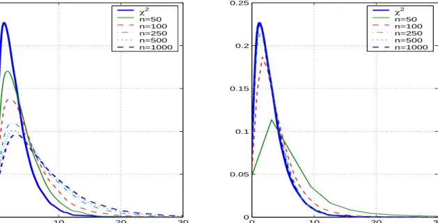
Fig. 1 compares two RESET tests–before and after bias corrections–whenXtandYtare linearly

cointegrated. The four graphs summarize the test performance underH0 from Table 1 with (a)

varying number of observations for a given level of serial correlation and (b) varying level of serial correlation for a given number of observations. As shown in the upper panels (a), with a moderate level of serial correlation (AR coefficient is 0.6) in the regression error, the RESET test without correction terms shows severe size distortions that become even worse as the sample size increases.4 For a nominal asymptotic 5% size, the actual probabilities of a type I error are 0.1058 (n=50), 0.1837 (n=100), 0.2817 (n=250), 0.3287 (n=500) and 0.357 (n=1000). This weakness of the RESET test is already well known in the stationary and highly autocorrelated Xt case

from work of Porter & Kashyap (1984), and the results here for the case of a cointegrating 4_{The probability of a type I error increases when the regression errors are more serially correlated as shown}

in (b). In the extreme case of (independent) I(1) errors, the test statistic diverges, as reported in Kim, Lee & Newbold (2003).

relation may be regarded as an extreme version of these earlier findings. While the test without correction terms suffers from increasing type I errors, the modified RESET test in the right panel of Fig. 1 (a) exhibits only a small size distortion, which vanishes as n increases, and at the same time, shows a relatively fast convergence to the limit distribution. The probabilities of the type I errors for the nominal 5% test are 0.1932 (n=50), 0.0926 (n=100), 0.0483 (n=250), 0.0496 (n=500) and 0.0491 (n=1000).

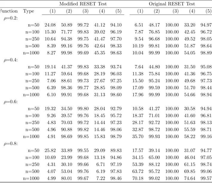
Fig. 1 (b) shows how the bias correction terms work for different ρ values. The left panel confirms the severe size distortions due to the serially correlated errors. For a nominal asymptotic 5% size, the probability of a type I error reaches up to 70% for ρ = 0.8, while including two correction terms bring it back to 4.99%. These figures are based on Table 1 which compares two tests for differentρ’s andn’s with k= 3.

4.2 Power of the Test

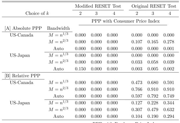
Table 1 also reports the power of the modified RESET test against some specific nonlinear models. With linear cointegration as the reference case in (1), simulation results show that the modified RESET test is quite sensitive to all the nonlinearities except (4) for a wide range ofρ

values. The probabilities of rejecting the linearity null are over 90% in most cases except for (4). As expected, the modified RESET test is most powerful against polynomial type nonlinearity (always higher than 99% in case (3)) but also shows good powers against logarithmic (2) and threshold (5) nonlinearities. Note also that the original RESET test in the second part also shows the similar pattern.

The low power against (4) is due to fact that the regression function is an integrable transform ofXt,which is poorly captured by the polynomial basis terms in the RESET test. In particular,

the asymptotic form of the function e−X2t whenX_t=O_p¡√t¢for larget is not captured by the

asymptotic form of the polynomial terms X_tj =Op

¡

tj/2¢in the RESET basis.

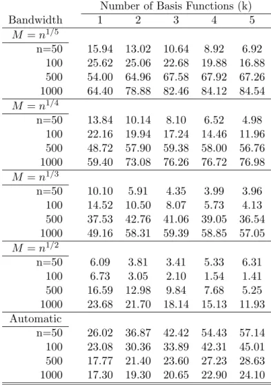
Table 2 shows the probability of rejecting the linear cointegration null hypothesis when the modified test is applied to two I(1) variables that are not cointegrated, i.e.

Y_t= 1.1X_t+u_t withu_t∼I(1)

As discussed in Theorem 7, the modified test statistic diverges at the raten/M so that the rejection rate is sensitive to the choice of the bandwidth parameter M. We report five cases, corresponding to M = n1/5_{, M = n}1/4_{, M = n}1/3_{, M = n}1/2 _{and the usual data-dependent}

automatic bandwidth (Andrews, 1991) for a Parzen kernel in Table 2. Two aspects of the results in Table 2 confirm Theorem 7. First, the rejection probability tends to higher for the smaller bandwidth choices for given k andn. Second, the rejection probability increases with nas well as with the number of augmented regressorskin general, espeically for smaller bandwidths. For

M =n1/3, the effect of increasingk on the rejection probability is not as large as in the case of

M =n1/5_{,and even decreases for M =n}1/2_{. When an automatic bandwidth rule is employed,}

increasingkhas a more significant effect on power for a givennthan increasingnfor a givenk.

4.3 Limitations and Practical Issues

The limitations of the modified RESET test are related to the approximation method that the test is based on and the nature of the nonlinear cointegration functional forms. As mentioned

previously, once the nonlinear cointegrating function is given, the size of the approximation error is determined by the type and number of the basis functions {Fj}kj=1. These choices

determine how well a linear combination of the basis functions can approximate some nonlinear cointegrating function ofXt.If there exists a set of coefficient

©

β_jªk_j=1 such thatP_jk₌₁β_jFj(Xt)

is close to f(Xt) over a wide enough domain (since an I(1) process like Xt visits all points of

the space an infinite number of times), then we can expect the test to reject linear cointegration in favor of some form of nonlinear cointegration, corresponding to the non-zero ©β_jªestimates. Once the basis functions {Fj}kj=1 are selected, k needs to be chosen. While larger k may

produce an improved approximation to f(·), in a finite sample testing framework there exist some trade-offs. On the one hand, larger values ofk will, at least to a certain point5, generally increase the power of the test by virtue of their improved approximation capability. On the other hand, larger k increases the risk of spurious nonlinearity resulting in a higher probability of a type I error under the null. Moreover, to reject the null hypothesisH₀:β₁=· · ·=β_k = 0, at least one significant coefficient will suffice, a condition that is less restrictive than requiring a good fit to f(Xt) by

P_k

j=1βˆjFj(Xt). Simulations (not reported here) suggests that the use

of k= 2 or 3 generally produces good size and reasonable power, while increasing ktok= 3 or 4 adds power without too much compromise in size.

Although not shown explicitly in the regression equation (2), the choice of bandwidth pa-rameterM for kernel estimation of long-run (co)variance can be another important element that affects the size and the power of the test, especially in small sample. As discussed in Theorem 7 and shown in Table 2, the power against the no-cointegration alternative depends on n/M. The test statistic under the some alternatives diverges faster asM/nbecomes smaller, but this makes the test statistic under the null converge to the asymptotic distribution at a slower rate. Therefore, in addition to the choice of k, it is recommended to apply the test with different combinations of kand M to get more a concrete result.

One popular choice for the bandwidth selection is the data dependent method in Andrews (1991). He proposes the automatic bandwidth choices for various kernels, and for the Parzen kernel we use, the automatic bandwidth is

M = 2.6614 · n·µX 4ˆρ 2_ˆσ2 (1−ρˆ)8 ¶ µX σˆ 4 (1−ˆρ)4 ¶¸1/5

where ˆρ is the AR(1) coefficient estimate in ˆut=ρuˆt−1+et and ˆσ2 is the variance estimate of

et.

Another important factor that affects the power of the test is the actual nonlinear functional form. Although general approximation methods, including the power series approximations that underlie the RESET test, can provide reasonable approximations to a wide class of nonlinear functions, there are nonlinear transformations that cannot be well approximated by these meth-ods. In particular, certain extensions to polynomial (or rational) approximants are generally needed in order to produce global approximations to functions over the whole real line. Phillips (1983) suggested a class of extended rational approximants that have good global approximant 5_{For k very large, the regressor matrix F can manifest multicollinearity and principal components may be}

used. In many cases, the first few principal components tend to explain most of variation in F and increasing k then leads to little improvement in the power of the test. Note that increasing k also leads to a decrease in degrees of freedom in the regression.

performance over the whole real line to integrable functions. One has to keep in mind that ac-cepting the null of linear cointegration leaves open the possibility of some undetected nonlinear effects (especially if these are of the ‘small’ type that would be delivered by integrable transfor-mations). Rejecting the null suggests that there may be nonlinear models that outperform the linear model or that there may be no meaningful cointegrating relation.

Estimated linear combinations of the basis functions can suggest a possible nonlinear alter-native if the true relationship is nonlinear. In this case, as discussed in the previous section, the modified RESET test can be interpreted as an LM test which compares a linear cointegra-tion model against an estimated approximacointegra-tion to some unknown nonlinear cointegracointegra-tion model. When the test rejects the null, we can write down an alternative nonlinear model with additional basis functions and re-estimate this model using FM regression. This leaves the remaining issues of choosing a suitable value of k for the regression so that the approximation error is reduced while not attempting to overfit the data. These issues are complex and are beyond the scope of the present paper.6

5

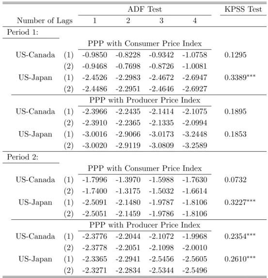
Empirical Application to PPP

The introduction of unit root limit theory and cointegration methods have led to a vast number of empirical studies with nonstationary time series, many of them conducted without further attention to specification testing beyond what is implied by unit root and cointegration tests. This section considers the purchasing power parity (PPP) relationship between nominal exchange rates and the foreign-domestic price ratio and applies the modified RESET linearity test to check whether the traditional linear cointegration specification is appropriate in this context.

5.1 PPP Models

PPP is a simple, intuitively appealing empirical proposition dated at least to the sixteenth century in Spain (Dornbusch, 1987). The theory postulates that once converted to a common currency, the price level of traded goods should be equalized across countries due to arbitrage. In this strict sense, the idea is sometimes understood as an extension of the law of one price (LOP). For a nominal exchange rate,St, a domestic price of a traded good iat timet,Pi,t, and

the foreign price for the same good, P∗

i,t, the LOP states that the same good should be sold at

the same price in different countries if prices are converted into a common currency (Rogoff, 1996)

P_i,t =S_t·P_i,t∗.

Aggregating this relationship over traded goods, PPP states that X i Pi,t=St· X i P_i,t∗.

For a variety of reasons, this exact form of PPP, the so-called absolute PPP, does not hold and a weaker version of PPP is commonly used to provide a definition of the real exchange rate as

qt=st+p∗t−pt,

6_{Of course, rejecting the null of linear cointegration may be due either to nonlinearity or to lack of}

cointegra-tion. Developing an approximate nonlinear cointegrated system will be valid only when the rejection is due to nonlinearity.

where q_t and s_t are log transforms of real and nominal exchange rates, and p∗

t and pt are log

transforms of foreign and domestic price levels.

Intuitively accepted as providing a long-run equilibrium relationship among price levels and exchange rates, PPP has been tested in various frameworks, leading to some mixed empirical findings.7 There have been many attempts to explain, using both economic and statistical arguments, the failure to find concrete empirical evidence for PPP.8 _{For example, in the weaker}

version of PPP, the log of the real exchange rate qt is usually divided into two parts: a traded

goods component and a bilateral difference between the relative price of traded to non-traded goods, viz., qt=st+p∗t−pt= © st+pTt∗−pTt ª +©α∗(pN_t ∗−p_tT∗)−α(pN_t −pT_t)ª

where the superscripts ‘T’ and ‘N’ stand for ‘traded’ and ‘non-traded’ respectively. The price indices are generally assumed to be geometric averages of traded and non-traded goods,

pt= (1−α)ptT +αpNt and p∗t = (1−α∗)pTt∗+α∗pNt ∗,

and, defining

P1 =st+pTt∗−ptT and P2 =α∗(ptN∗−pTt∗)−α(pNt −pTt),

the real exchange rate is stationary either if P1 and P2 are stationary, or if P1 and P2 are nonstationary but cointegrated. Accepting PPP as a long-run equilibrium relationship, P1 is stationary and it is not at all surprising that many find the real exchange rate to be nonstationary considering the presence of the possibly nonstationary componentP2.

Traditional unit root/cointegration approaches have been the most widely used method in PPP empirical studies, but these methods have often failed to find any strong support for PPP. These failures have led to the use of many new methods in searching for evidence of PPP, including longer datasets, panel unit root evaluations, and the use of nonlinear models. Noticing the low power of unit root tests in small samples, researchers have tested PPP using long-horizon data, finding stronger support for PPP (e.g. Lothian & Taylor, 1995) by this method. Many empirical researchers have found that the floating exchange rate system introduced with the Bretton Woods system has led to larger deviations from PPP (e.g. Taylor, 2002). Using cross-country data to improve the power of unit root tests has also tended to produce stronger support for PPP, but these methods have also been criticized by O’Connell (1998) and others for neglecting cross country dependence. While these first two methods have involved the use of different datasets to improve tests of PPP, the last approach takes into account the possibility of different model specifications. Nonlinear specifications are often obtained from market frictions like transaction costs, e.g. Dumas (1992), Sercu, Uppal & van Hulle (1995), and Michael, Nobay & Peel (1997). Because of market frictions, there exists an inactive range around parity in which international arbitrage does not work and adjustments to parity start to occur only when the exchange rate moves out of this range. This nonlinear adjustment to parity can be formulated using variations of the threshold model (e.g. STAR, ESTAR) and some significant empirical 7_{Froot & Rogoff (1995) provide a discussion of the evolution of PPP tests and Rogoff (1996) surveys empirical}

studies in the area.

8_{See Grilli & Kaminsky (1991), Pedroni (2001) and Ng & Perron (2002) for some statistical arguments and}