Multivariate Normal Mixture GARCH

No. 2006/09

Multivariate Normal Mixture GARCH

Markus Haas, Stefan Mittnik,

and Marc S. Paolella

Center for Financial Studies

The

Center for Financial Studies

is a nonprofit research organization, supported by an

association of more than 120 banks, insurance companies, industrial corporations and

public institutions. Established in 1968 and closely affiliated with the University of

Frankfurt, it provides a strong link between the financial community and academia.

The CFS Working Paper Series presents the result of scientific research on selected

topics in the field of money, banking and finance. The authors were either participants

in the Center´s Research Fellow Program or members of one of the Center´s Research

Projects.

If you would like to know more about the

Center for Financial Studies

, please let us

know of your interest.

* We thank participants of the 2005 NBER/NSF Satellite Workshop \Financial Risk and Time Series Analysis" in Munich for helpful comments and suggestions. The research of M. Haas und S. Mittnik was supported by the Deutsche Forschungsgemeinschaft (SFB 386). Part of the research of M. S. Paolella has been carried out within the National Centre of Competence in Research \Financial Valuation and Risk Management" (NCCR FINRISK), which is a research program supported by the Swiss National Science Foundation. Address correspondence to Stefan Mittnik, Chair of Financial Econometrics, Institute of Statistics, University of Munich, D-80799 Munich, Germany, or e-mail: [email protected].

1 _{Institute of Statistics, University of Munich}

2 _{Institute of Statistics, University of Munich, Center for Financial Studies, Frankfurt, and Ifo Institute for Economic Research, Munich}

CFS Working Paper No. 2006/09

Multivariate Normal Mixture GARCH*

Markus Haas

, Stefan Mittnik

,

and Marc S. Paolella

April 2006

Abstract:

We present a multivariate generalization of the mixed normal GARCH model proposed in

Haas, Mittnik, and Paolella (2004a). Issues of parametrization and estimation are discussed.

We derive conditions for covariance stationarity and the existence of the fourth moment, and

provide expressions for the dynamic correlation structure of the process. These results are also

applicable to the single-component multivariate GARCH(p, q) model and simplify the results

existing in the literature. In an application to stock returns, we show that the disaggregation of

the conditional (co)variance process generated by our model provides substantial intuition,

and we highlight a number of findings with potential significance for portfolio selection and

further financial applications, such as regime-dependent correlation structures and leverage

effects.

JEL Classification: C32, C51, G10, G11

Keywords: Conditional Volatility, Regime-dependent Correlations, Leverage Effect,

Multivariate GARCH, Second-order Dependence

Non–technical Summary

In this paper, we propose a multivariate generalization of the normal mixture GARCH model originally proposed in Haas, Mittnik, and Paolella (2004a, an earlier version has also been published as CFS Working Paper 2002/10). One of the most characteristic properties of this model is that it explicitly allows the evolution of risk inherent in a given financial position to depend on—unobservable—states of the market, such as, for example, bull and bear markets. This meets frequently expressed concerns about standard GARCH models, which are not able to capture state–dependent volatility dynamics.

As shown in Alexander and Lazar (2004, 2005), and Haas, Mittnik, and Paolella (2004a,b) for a considerable number of financial return series, the normal mixture GARCH model is well suited for modeling and forecasting the volatility of financial assets such as stocks and currencies, and consistently outperforms many competing approaches both in– and out–of– sample. However, while the existing literature on normal mixture GARCH models is confined to univariate processes, many applications in finance are inherently multivariate and require us to understand the dependence structure between assets. For example, in portfolio man-agement, correlations between assets are often of predominant interest, because the size of the correlations determines the degree of risk reduction which can be achieved by efficient portfolio diversification. However, there is evidence that stock returns exhibit stronger de-pendence in bear markets, when volatility is high and market returns are decreasing. This issue is of considerable importance for portfolio selection and risk management, because it is in times of adverse market conditions that the benefits from diversification are most urgently needed. Models not taking into account the state–dependent correlation structure will thus tend to overstate the benefits of diversification in bear markets, and, consequently, they will underestimate the risk during such periods.

We discuss this and further implications of the mixture approach to multivariate GARCH models in the paper, and demonstrate their empirical relevance in an application to stock mar-ket returns. Moreover, we address issues of parametrization, estimation, and model selection, and we derive various relevant dynamic properties of the multivariate normal mixture GARCH process.

Nichttechnische Zusammenfassung

Die vorliegende Arbeit ist einer multivariaten Verallgemeinerung des sog. Normal Mixture

GARCH Modells gewidmet, dessen univariate Variante von Haas, Mittnik und Paolella (2004a, siehe auch CFS Working Paper 2002/10) vorgeschlagen wurde. Dieses Modell unterscheidet sich von traditionellen GARCH–Ans¨atzen insbesondere dadurch, dass es eine Abh¨angigkeit der Risikoentwicklung von – typischerweise unbeobachtbaren – Marktzust¨anden explizit in Rech-nung stellt. Dies wird durch die Beobachtung motiviert, dass das weit verbreitete GARCH Modell in seiner Standardvariante auch dann keine ad¨aquate Beschreibung der Risikodynamik leistet, wenn die Normalverteilung durch flexiblere bedingte Verteilungen ersetzt wird. Zus-tandsabh¨angige Volatilit¨atsprozesse k¨onnen etwa durch die variierende Dominanz heterogener Marktteilnehmer oder durch wechselnde Marktstimmungen ¨okonomisch zu erkl¨aren sein.

Anwendungen des Normal Mixture GARCH Modells auf zahlreiche Aktien– und Wech-selkurszeitreihen (siehe z.B. Alexander und Lazar, 2004, 2005; und Haas, Mittnik und Paolella, 2004a,b) haben gezeigt, dass es sich zur Modellierung und Prognose des Volatilit¨atsprozesses der Renditen solcher Aktiva hervorragend eignet. Indes beschr¨anken sich diese Analysen bisher auf die Untersuchung univariater Zeitreihen. Zahlreiche Probleme der Finanzwirtschaft er-fordern jedoch zwingend eine multivariate Modellierung, mithin also eine Beschreibung der Abh¨angigkeitsstruktur zwischen den Renditen verschiedener Wertpapiere. Insbesondere f¨ur solche Analysen erweist sich der Mischungsansatz aber als besonders vielversprechend. So spielen etwa im Portfoliomanagement die Korrelationen zwischen einzelnen Wertpapierren-diten eine herausragende Rolle. Die St¨arke der Korrelationen ist von entscheidender Bedeu-tung daf¨ur, in welchem Ausmaß das Risiko eines effizienten Portfolios durch Diversifikation reduziert werden kann. Nun gibt es empirische Hinweise darauf, dass die Korrelationen etwa zwischen Aktien in Perioden, die durch starke Marktschwankungen und tendenziell fallende Kurse charakterisiert sind, st¨arker sind als in ruhigeren Perioden. Das bedeutet, dass die Vorteile der Diversifikation in genau jenen Perioden geringer sind, in denen ihr Nutzen am gr¨oßten w¨are. Modelle, die die Existenz unterschiedlicher Marktregime nicht ber¨ucksichtigen, werden daher dazu tendieren, die Korrelationen in den adversen Marktzust¨anden zu unter-sch¨atzen. Dies kann zu erheblichen Fehleinsch¨atzungen des tats¨achlichen Risikos w¨ahrend solcher Perioden f¨uhren.

Diese und weitere Implikationen des Mischungsansatzes im Kontext multivariater GARCH Modelle werden in der vorliegenden Arbeit diskutiert, und ihre Relevanz wird anhand einer empirischen Anwendung dokumentiert. Er¨ortert werden ferner Fragen der Parametrisierung und Sch¨atzung des Modells, und einige relevante theoretische Eigenschaften werden hergeleitet.

1

Introduction

Since the publication of Engle’s (1982) ARCH model and its generalization to GARCH by Bollerslev (1986), a considerable amount of research has been undertaken to develop models that adequately capture the volatility dynamics observed in financial return data at weekly, daily or higher frequencies. Within the GARCH class of models, the recently proposed family of normal mixture GARCH processes (Alexander and Lazar, 2004; Haas, Mittnik, and Paolella, 2004a,b) has been shown to be particularly well suited for analyzing and forecasting short– term financial volatility.1 _{A finite mixture of a few normal distributions, say two or three, is}

capable of capturing the skewness and kurtosis detected in both conditional and unconditional return distributions, and can, when coupled with GARCH–type equations for the component variances, exhibit quite complex dynamics, as often observed in financial markets. For example, there may be components driven by nonstationary dynamics, while the overall process is still stationary. This corresponds to the observation that markets are stable most of the time, but, occasionally, subject to severe, short–lived fluctuations. Empirical results for several stock and exchange rate return series, as reported in Alexander and Lazar (2004, 2005), and Haas, Mittnik, and Paolella (2004a,b) show that the normal mixture GARCH process provides a plausible disaggregation of the conditional variance process, and that it performs well in out– of–sample density forecasting, which can be viewed as a rigorous check of model adequacy.

While the existing literature on normal mixture GARCH models is confined to univariate processes, many applications in finance are inherently multivariate and require us to under-stand the dependence structure between assets. For example, in applications to portfolio selection, correlations between assets are often of predominant interest. However, there is evidence that asset correlations are regime–dependent, in the sense that stock returns appear to exhibit stronger dependence during periods of high volatility, which are often associated with market downturns (see, for example, Patton, 2004). As stressed by Campbell, Koedijk, and Kofman (2002), the issue of regime–dependent correlations is of considerable interest for portfolio analysis, because it is in times of adverse market conditions that the benefits from diversification are most urgently needed.

In this paper, we generalize the normal mixture GARCH model proposed by Haas, Mittnik, and Paolella (2004a) to the multivariate setting. We will define the model in terms of the

1

These models are generalizations of earlier proposed applications of normal mixture distributions in the GARCH context (see Vlaar and Palm, 1993; Palm and Vlaar, 1997; and Bauwens, Bos, and van Dijk, 1999). There is also some relationship with the models of Wong and Li (2001), and Cheung and Xu (2003), as well as with the Markov–switching (G)ARCH models of Cai (1994), Hamilton and Susmel (1994), Gray (1996), Dueker (1997), and Klaassen (2002). A detailed discussion of these models and their relationships is provided in Haas, Mittnik, and Paolella (2004a,b).

arguably most general multivariate GARCH specification, i.e., the vech model as defined by Bollerslev, Engle, and Wooldridge (1988). This model, without further restrictions, is not amendable for direct estimation, but it nests several more practicable specifications, such as the diagonal vech model, also proposed by Bollerslev, Engle, and Wooldridge (1988), and the BEKK model of Engle and Kroner (1995).2

For the multivariate normal mixture GARCH(p, q) model, we present conditions for covari-ance stationarity and the existence of the fourth unconditional moment, along with expres-sions for the autocorrelation matrices of the squared process. As the mixture model nests the single–component specification, these results are also applicable to the standard multivariate GARCH(p, q) model in vech form. For this model, our results improve upon the existing lit-erature on this issue, both in terms of simplicity and interpretability, as will be discussed in Appendix D. Moreover, no results for asymmetric multivariate GARCH models, i.e., specifi-cations with a leverage effect, exist in the literature so far.

In the most general specification of our model, we allow for leverage effects, i.e., an asym-metric reaction of variances and covariances to positive and negative shocks, as well as for asymmetry of the conditional mixture density. The second– and fourth–order moment struc-ture for this general specification is detailed for the empirically most relevant GARCH(1,1) model.

The paper is organized as follows. In Section 2, we define the model and present results on its unconditional moments and its dynamic correlation structure. In Section 3, we provide an application to a bivariate stock return series. Section 4 concludes and identifies issues for further research. Technical details are gathered in a set of appendices.

2

The Model and its Properties

In this section, we define the multivariate normal mixture GARCH process, discuss estimation issues and present some theoretical properties.

2.1 Finite Mixtures of Multivariate Normal Distributions

AnM–dimensional random vectorXis said to have ak–component multivariate finite normal mixture distribution, or, in short, MNM(k), if its density is given by

f(x) = k X j=1 λjφ(x;µj, Hj), (1) 2

whereλj >0,j= 1, . . . , k,Pjλj = 1, are the mixing weights, and φ(x;µj, Hj) = 1 (2π)M/2p |Hj| exp −1 2(x−µj) 0_H−1 j (x−µj) , j= 1, . . . , k, (2) are the component densities. The normal mixture random vector has finite moments of all orders, with expected value and covariance matrix given by (see, e.g., McLachlan and Peel, 2000) E(X) = k X j=1 λjµj, (3) and Cov(X) = k X j=1 λj(Hj +µjµ0j)−   k X j=1 λjµj     k X j=1 λjµj   0 (4) = k X j=1 λjHj+ k X j=1 λj(µj −E(X))(µj−E(X))0,

respectively. We will also make use the third and fourth moments of a multivariate normal mixture distribution, which are given in Appendix B.

A question that naturally arises in the estimation of mixture distributions is identifiability. Obviously, a lack of identification always arises as a consequence of label switching, but this can be ruled out by restricting the parameter space such that no duplication appears, e.g., by imposing λ1 > λ2 > · · · > λk. However, there is a more fundamental problem when the

class of density functions to be mixed is linearly dependent (Yakowitz and Spragins, 1968). Fortunately, the class of multivariate finite normal mixtures is identifiable, as has been shown by Yakowitz and Spragins (1968), who generalized Teicher’s (1963) results for univariate finite normal mixtures.

An issue which has not been satisfactorily resolved so far is the empirical determination of the number of mixture components, i.e., the choice ofkin (1). It is well–known that standard test theory breaks down in this context (McLachlan and Peel, 2000). However, there is some evidence, that, at least for unconditional mixture models, the Bayesian information criterion of Schwarz (1978) provides a reasonably good indication for the number of components (see McLachlan and Peel, 2000, Ch. 6, for a survey and further references). According to Kass and Raftery (1995), a BIC difference of less than two corresponds to “not worth more than a bare mention”, while differences between two and six imply positive evidence, differences between six and ten give rise to strong evidence, and differences greater than ten invoke very strong evidence.

2.2 Multivariate Normal Mixture GARCH Processes

The M–dimensional time series {t} is said to be generated by a k–component multivariate

normal mixture GARCH(p, q) process, or, in short, MNM(k)–GARCH(p, q), if its conditional distribution is ak–component multivariate normal mixture, denoted as

t|Ψt−1 ∼MNM(λ1, . . . , λk, µ1, . . . , µk, H1t, . . . , Hkt), (5)

where Ψt is the information set at time t. By imposing µk=−Pkj=1−1(λj/λk)µj on the mean

of the kth component it is guaranteed that t in (5) has zero mean. Furthermore, stack the

N :=M(M+ 1)/2 independent elements of the covariance matrices and the “squared”t(i.e.,

t0t) inhjt := vech(Hjt),j= 1, . . . , k, andηt:= vech(t0t), respectively. Then, the component

covariance matrices evolve according to

hjt =A0j+ q X i=1 Aij˜ηij,t−i+ p X i=1 Bijhj,t−i, j= 1, . . . , k, (6)

where ˜η_ij,t = vech[(t−θij)(t−θij)0]; θij, i = 1, . . . , q, and A0j are columns of length M

and N, respectively; and Aij, i = 1, . . . , q, and Bij, i = 1, . . . , p, are N ×N matrices, j =

1, . . . , k. The θij’s are introduced in order to allow for the leverage effect in applications to

stock market returns, i.e., the strong negative correlation between equity returns and future volatility. In the univariate GARCH literature, various specifications of the leverage effect exist. Our choice, i.e., incorporating theθij’s in (6), can be viewed as a generalization of one

of the earliest versions, namely Engle’s (1990) asymmetric GARCH (AGARCH) model.3 In the univariate framework, this model has been coupled with the normal mixture GARCH structure by Alexander and Lazar (2005). We will denote the asymmetric MNM(k)–GARCH(p, q) as MNM(k)–AGARCH(p, q). Moreover, in some applications, a symmetric conditional density will be appropriate, so that, in (5),µ1 =· · ·=µk= 0. We will denote this restricted version as

MNMS(k)–(A)GARCH(p, q). An overview over the different model specifications is provided

in Table 1.

To compactify the notation and facilitate the theoretical analysis of the model, note that, by (A.3) in Appendix A, vech(t−iθ0ij+θij0t−i) = 2D+Mvec(θij0t−i) = 2D+M(IM⊗θij)t−i. Then

we rewrite (6) as hjt = ˜A0j+ q X i=1 Aijηt−i− q X i=1 Θijt−i+ p X i=1 Bijhj,t−i, j = 1, . . . , k, (7)

where ˜A0j := A0j +Pqi=1Aijvech(θijθij0 ), and Θij := 2AijDM+(IM ⊗θij), j = 1, . . . , k,

i = 1, . . . , q. Let ht := (h01t, . . . , h0kt)0; ˜A0 = ( ˜A001, . . . ,A˜00k)0; Θi = (Θi01, . . . ,Θ0ik)0, Ai =

3

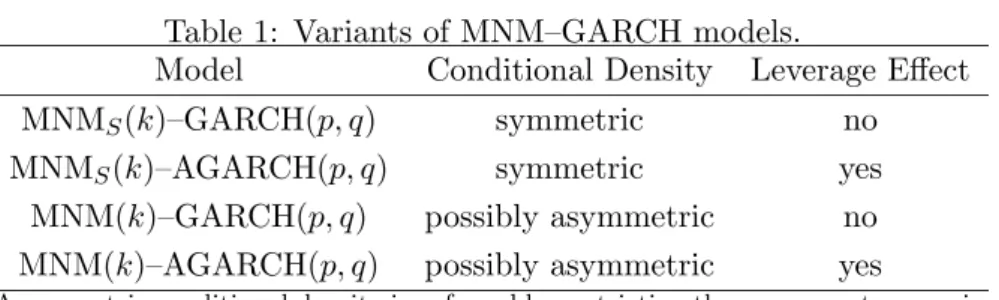
Table 1: Variants of MNM–GARCH models.

Model Conditional Density Leverage Effect MNMS(k)–GARCH(p, q) symmetric no

MNMS(k)–AGARCH(p, q) symmetric yes

MNM(k)–GARCH(p, q) possibly asymmetric no MNM(k)–AGARCH(p, q) possibly asymmetric yes

A symmetric conditional density is enforced by restricting the component means in (5) to zero, i.e.,µ1=· · ·=µk= 0; while the absence of a leverage effect is imposed

by restricting theθij’s in (6) to zero, i.e.,θij= 0,j= 1, . . . , k,i= 1, . . . , q.

(A0_i1, . . . , A0_ik)0, i = 0, . . . , q; and Bi = Lk_j=1Bij, i = 1, . . . , p, where L denotes the matrix

direct sum. Using these definitions, we have

ht= ˜A0+ q X i=1 Aiηt−i− q X i=1 Θit−i+ p X i=1 Biht−i. (8)

For estimation purposes, the general formulation as given in (6) is not directly applica-ble, and parameter constraints are required in order to guarantee positive definiteness of all conditional covariances matrices. A particular restriction of the vech form of the multivariate GARCH process, which guarantees positive definiteness, is implied by the BEKK model of Engle and Kroner (1995) which specifies the covariance matrices as

Hjt =A?0jA? 0 0j+ L X `=1 q X i=1 A?<sub>ij,`</sub>(t−i−θij)(t−i−θij)0A? 0 ij,`+ L X `=1 p X i=1 B<sub>ij,`</sub>? Hj,t−iB? 0 ij,`, j = 1, . . . , k, (9) whereA?_0j,j= 1, . . . , k, are triangular matrices. As shown by Engle and Kroner (1995), each BEKK model implies a unique vech representation (the converse is not true), and, once a BEKK representation (9) is estimated, the matricesAij andBij of the vech model (6) can be

recovered via Aij = L X `=1 D+<sub>M</sub>(A?<sub>ij,`</sub>⊗A?<sub>ij,`</sub>)DM, i= 1, . . . , q, j= 1, . . . , k, (10) Bij = L X `=1 D+_M(B_{ij,`</sub>? ⊗B<sub>ij,`}? )DM, i= 1, . . . , p, j= 1, . . . , k,

whereDM andDM+ denote the duplication matrix and its Moore–Penrose inverse, respectively,

both of which we briefly review in Appendix A. Thus, all results derived for the vech model are also applicable to the BEKK model. In practical applications, L = 1 is the standard choice, as well as p = q = 1. For this specification, it follows from Proposition 2.1 of Engle and Kroner (1995) that the model is identified if the diagonal elements ofA?_0j, as well as the top left elements of matrices A?_1j and B₁?_j, j = 1, . . . , k, are restricted to be positive. We

will thus impose these restrictions in the applications below. In addition, while, for L = 1, the BEKK model already involves fewer parameters than the unrestricted vech form, further simplifications can be obtained by assuming that A?_1j and B?_1j, j = 1, . . . , k, are diagonal matrices.

In the following discussion of the vech specification we will always assume that positive def-inite covariances matrices are guaranteed, without further specifying the constraints employed for achieving this.

2.3 Existence of Moments and Autocorrelation Structure

It is clear that, for practical purposes, the most important MNM(k)–AGARCH(p, q) process is the specification wherep=q= 1, which is defined by (5) and

ht= ˜A0+A1ηt−1−Θ1t−1+B1ht−1. (11)

For later reference, we summarize the dynamic properties of the process given by (5) and (11) in Proposition 1, while the corresponding results for the GARCH(p, q) specification, which require a considerable amount of additional notation, are developed in Appendix D.

We denote as ρ(A) the largest eigenvalue in modulus of a square matrix A, i.e.,

ρ(A) := max{|z|:zis an eigenvalue of A}, (12) and define the vector of mixing weightsλ= (λ1, . . . , λk)0. Following the classic papers of Engle

(1982) and Bollerslev (1986), we assume for simplicity that the process starts indefinitely far in the past with finite fourth moments.

Proposition 1 The MNM(k)–AGARCH(1,1) process given by (5) and (11) is covariance stationary if and only ifρ(C11)<1, where the kN×kN matrix C11 is defined by

C11=λ0⊗A1+B1. (13)

In this case, the unconditional expectation of vectorhtis E(ht) = (IkN−λ0⊗A1−B1)−1[ ˜A0+

A1(λ0⊗IN)˜µ], where µ˜ is defined in Lemma 4 in Appendix B.1; and the unconditional

expec-tation ofηtis(λ0⊗IN)(E(ht) + ˜µ). Moreover, the unconditional fourth moment E(ηtηt0) exists

if and only if ρ(C22)<1, where C22 is the (kN)2×(kN)2 matrix given by

C22= (A1⊗A1)GM(IN ⊗vec(Λ)0⊗IN)(KN k⊗IkN) + 2NkN(B1⊗λ0⊗A1) +B1⊗B1. (14)

In (14),GM is the N2×N2 matrix defined in (B.13) in Appendix B.2, Λ =diag(λ1. . . , λk),

Kmn is the commutation matrix defined in Appendix A, andNn= (In2 +K_nn)/2. An

expres-sion for the fourth–moment matrix is given in Appendix C.1. Ifρ(C22)<1 holds, the

given by

Γτ = (λ0⊗IN)C11τ−1Q, (15)

where Q is a constant matrix given in (C.21) in Appendix C.2.

The results of Proposition 1 are derived in Appendices B and C. From (15), the autocor-relation matrices,Rτ, can be calculated in the usual way. I.e., ifD is a diagonal matrix with

the square roots of diag(Γ0) on its diagonal, where Γ0 := E(ηtη0t)−E(ηt)E(ηt)0, then

Rτ =D−1ΓτD−1. (16)

Note that the term determining the rate of decay of Γτ is C11τ . Thus, under covariance

stationarity, the largest eigenvalue in magnitude of the matrixC11 defined in (13) can be used

as a measure for the persistence of shocks to volatility.

It may be worth pointing out that conditions (13) and (14), as well as the speed of decline of the autocorrelation function, do not depend on the “leverage terms”θ1j in (6). Moreover,

the stationarity conditionρ(C11)<1, whereC11is defined in (13), allows some components to

be nonstationary, in the sense that the covariance stationarity condition for single–component multivariate GARCH(1,1) processes, i.e.,4

ρ(A1j+B1j)<1, (17)

is not satisfied for these components. Nevertheless, the overall process can still be stationary, as long as the corresponding mixture weights are sufficiently small. This parallels the situation in the univariate case (see Alexander and Lazar, 2004; and Haas, Mittnik, and Paolella, 2004a,b), and will be empirically illustrated in Section 3.

3

Application to Stock Market Returns

We investigate the bivariate time series of daily returns of the NASDAQ and the Dow Jones Industrial Average (DJIA) indices from January 1990 to December 1999, a sample of T = 2516 observations.5 _{Continuously compounded percentage returns are considered, i.e., r}

it =

100×log(Pit/Pi,t−1), i = 1,2, where Pit denotes the level of index i at time t. We let r1t

and r2t denote the time–t return of the NASDAQ and the DJIA, respectively. As we want

to concentrate our analysis on the volatility dynamics, a univariate linear AR(1) filter was applied to the series in order to remove (weak) low–order autocorrelation. Subsequently, all

4

For this condition, see Bollerslev and Engle (1993), and Engle and Kroner (1995).

5

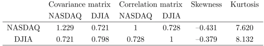
Table 2: Descriptive statistics of the filtered NASDAQ/DJIA returns. Covariance matrix Correlation matrix Skewness Kurtosis NASDAQ DJIA NASDAQ DJIA

NASDAQ 1.229 0.721 1 0.728 –0.431 7.620 DJIA 0.721 0.798 0.728 1 –0.379 8.132

“Skewness” and “Kurtosis” refer to the standardized third and fourth moments, respectively. That is, Skewness =m3/m

3/2

2 , and Kurtosis =m4/m22, wheremi is theith central moment

(about the mean).

results are for the filtered version of the data. A few descriptive statistics of the filtered series are summarized in Table 2.

To make sure that all conditional covariance matrices are positive definite, we use the BEKK parametrization (9). Several versions of the general mixture GARCH model (5)–(6) withp=q= 1 have been estimated. Namely, the single–component model, which corresponds tok= 1 in (1), and which is just the standard Normal–GARCH process, has been estimated with and without imposing a symmetric reaction to negative and positive shocks. The first of these models, where θ11= 0 in (6), will be denoted by Normal–GARCH(1,1), and the second

by Normal–AGARCH(1,1). Also, two–component models are considered with and without symmetric conditional mixture densities, i.e., with and without imposingµ1 =µ2 = 0 in (5),

as well as with and without leverage effects. To refer to these different models, we will use the typology of Table 1.

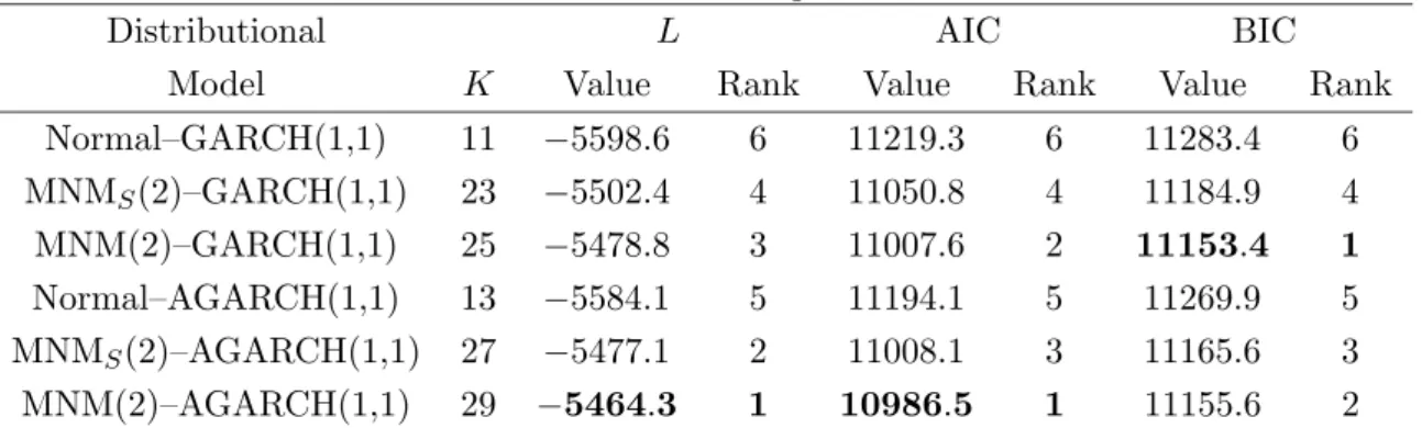
Table (3) reports likelihood–based goodness–of–fit measures for the models and their rank-ings with respect to each of these criteria, i.e., the value of the maximized log–likelihood function, and the AIC and BIC criteria of Akaike (1973) and Schwarz (1978), respectively.

While it is not surprising that the Normal–GARCH model is the worst performer with re-spect to each of these criteria, several additional observations are worth mentioning. First, the normal mixture specifications allowing for asymmetric conditional densities, i.e., admitting nonzero component means in (5), are always favored against their symmetric counterparts. This is not the case when we consider the dynamic asymmetry, i.e., the asymmetric reac-tion of future variances to negative and positive shocks. The improvement in log–likelihood is much larger when passing from the symmetric MNMS(2)–GARCH(1,1) to the MNMS(2)–

AGARCH(1,1) model (difference in log–likelihood: 25.3), than when passing from the asym-metric MNM(2)–GARCH(1,1) process to its AGARCH(1,1) counterpart (difference in log– likelihood: 14.5). As a consequence, the MNM(2)–GARCH(1,1) specification performs best overall according to the BIC. We note, however, that the difference in BIC for the latter two models is close to being insignificant according to the Kass and Raftery–recommendation

Table 3: Likelihood–based goodness of fit.

Distributional L AIC BIC

Model K Value Rank Value Rank Value Rank Normal–GARCH(1,1) 11 −5598.6 6 11219.3 6 11283.4 6 MNMS(2)–GARCH(1,1) 23 −5502.4 4 11050.8 4 11184.9 4 MNM(2)–GARCH(1,1) 25 −5478.8 3 11007.6 2 11153.4 1 Normal–AGARCH(1,1) 13 −5584.1 5 11194.1 5 11269.9 5 MNMS(2)–AGARCH(1,1) 27 −5477.1 2 11008.1 3 11165.6 3 MNM(2)–AGARCH(1,1) 29 −5464.3 1 10986.5 1 11155.6 2

The leftmost column states the type of volatility model fitted to the bivariate NASDAQ/DJIA returns. The column labeledKreports the number of parameters of a model;Lis the log likelihood; AIC =−2L+ 2K; and BIC =−2L+KlogT, whereT is the number of observations. For each of the three criteria the criterion value and the ranking of the models are shown. Boldface entries indicate the best model for the particular criterion.

mentioned at the end of Section 2.1. Also, a closer inspection of the parameter estimates will reveal that the leverage effect may be an exclusive feature of the high–volatility component, so that the difference in the number of parameters between these models shrinks from four to two, which would reverse these conclusions.6

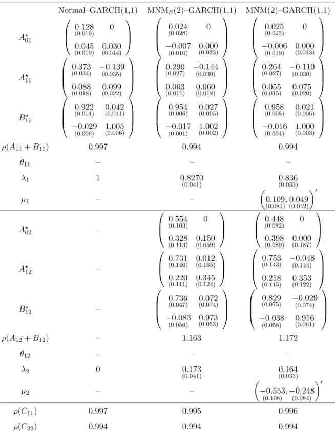
The maximum likelihood estimates are reported in Tables 4 and 5 for the models without and with leverage effect, i.e., dynamic asymmetry, respectively. Reported are the parameter matricesA?

0j,A?1j, andB1?j,j= 1,2, of the BEKK representation (9), from which the parameter

matrices of the vech representation, A1j and B1j, j = 1,2, can be recovered via (10). In

addition, we report the regime–specific persistence measures, i.e., the largest eigenvalues of the matricesA1j+B1j,j = 1,2, where these matrices have been computed from the BEKK

representation using (10), as well as the largest eigenvalues of the matricesC11andC22defined

in Proposition 1, which provide information about the existence of the unconditional second and fourth moments, respectively. The two–component models have been ordered such that

λ1 > λ2.

In discussing the parameter estimates, we first draw attention to a common characteristic of all mixture models fitted, whether they allow for asymmetry and/or leverage or not: All these models identify two components with distinctly different volatility dynamics. More precisely, the first component, i.e., the component with the larger mixing weight, is stationary in the sense that ρ(A11+B11) < 1, and it has less weight on the reaction parameters in A11 and

6

Alternatively, a likelihood ratio test for θ1 = θ2 = 0 could be conducted. The associated test statistic,

LRT = 2×(5478.8−5464.3) = 29, exceeds conventional critical values given by the asymptotically validχ2

Table 4: MNM–GARCH(1,1) parameter estimates for NASDAQ/DJIA returns Normal–GARCH(1,1) MNMS(2)–GARCH(1,1) MNM(2)–GARCH(1,1)

A?₀₁    0.128 (0.019) 0 0.045 (0.019) 0(0..030014)        0.024 (0.028) 0 −0.007 (0.016) 0(0..000023)         0.025 (0.025) 0 −0.006 (0.019) (00..000043)     A?₁₁     0.373 (0.034) −(00.035).139 0.088 (0.018) 0(0..099022)         0.290 (0.027) −(00..030)144 0.063 (0.011) (00..060018)         0.264 (0.027) −(00.030).110 0.055 (0.015) (00..075020)     B? 11     0.922 (0.014) (00..042011) −0.029 (0.006) (01..005006)         0.954 (0.006) 0(0..027005) −0.017 (0.001) 1(0..002002)         0.958 (0.008) (00..021006) −0.016 (0.004) (01..000003)     ρ(A11+B11) 0.997 0.994 0.994 θ11 – – – λ1 1 0.8270 (0.041) (00..836033) µ1 – – 0.109 (0.081),(00..049042) 0 A? 02 –    0.554 (0.103) 0 0.328 (0.113) (00..150059)       0.448 (0.082) 0 0.398 (0.089) (00..000187)    A? 12 –    0.731 (0.146) (00..012165) 0.220 (0.111) (00..345124)        0.753 (0.143) −(00.144).048 0.218 (0.115) (00..353122)     B₁₂? –     0.736 (0.047) 0(0..072074) −0.083 (0.056) 0.973 (0.053)         0.829 (0.075) −(00..074)029 −0.038 (0.058) (00..916061)     ρ(A12+B12) – 1.163 1.172 θ12 – – – λ2 0 0.173 (0.041) (00..164033) µ2 – – −0.553 (0.108) ,−0.248 (0.084) 0 ρ(C11) 0.997 0.995 0.996 ρ(C22) 0.994 0.994 0.994

Approximate standard errors are given in parentheses. Note that matrices A?0j, A?1j, and B1?j, j = 1,2,

correspond to the BEKK representation (9) of the model, while matricesA1j+B1j, j= 1,2, the maximal

eigenvalues of which are reported, are associated with the vech representation (6). ρ(C11) andρ(C22) denote

the largest eigenvalues of the matricesC11 and C22, defined in Proposition 1, which determine whether the

Table 5: MNM–AGARCH(1,1) parameter estimates for NASDAQ/DJIA returns

Normal–AGARCH(1,1) MNMS(2)–AGARCH(1,1) MNM(2)–AGARCH(1,1)

A?₀₁    0.135 (0.024) 0 0.046 (0.023) 0(0..031017)       0.000 (0.041) 0 0.000 (0.019) 0(0..000019)       0.000 (0.044) 0 0.000 (0.033) (00..000026)    A?₁₁     0.389 (0.038) −(00.037).135 0.094 (0.020) 0(0..108023)         0.288 (0.028) −(00.030).149 0.060 (0.015) 0(0..059020)         0.258 (0.012) −(00..017)114 0.052 (0.013) (00..068018)     B₁₁?     0.911 (0.017) (00..042014) −0.034 (0.008) (01..004007)         0.958 (0.007) (00..024006) −0.015 (0.004) (01..001003)         0.963 (0.002) (00..017002) −0.013 (0.002) (00..999002)     ρ(A11+B11) 0.996 0.998 0.996 θ11 0.305 (0.062),0(0..243079) 0 −0.113 (0.083),−(00.097).164 0 −0.116 (0.076) ,−(00.100).153 0 λ1 1 0.755 (0.036) (00..759033) µ1 – – 0.099 (0.032),(00..044019) 0 A?₀₂ –     0.132 (0.128) 0 −0.066 (0.080) (00..000170)         0.081 (0.117) 0 −0.088 (0.080) (00..000210)     A?₁₂ –    0.635 (0.094) 0(0..027097) 0.193 (0.078) 0(0..312074)        0.603 (0.059) −(00..071)046 0.143 (0.106) (00..310039)     B? 12 –     0.678 (0.075) (00..094071) −0.121 (0.049) (00..989039)         0.727 (0.048) (00..085046) −0.091 (0.030) (00..981027)     ρ(A12+B12) – 1.019 1.017 θ12 – 0.814 (0.127),(00..619161) 0 0.878 (0.114),(00..636138) 0 λ2 0 0.245 (0.036) (00..241033) µ2 – – −0.310 (0.068) ,−(00.055).140 0 ρ(C11) 0.996 0.994 0.996 ρ(C22) 0.993 0.991 0.992

more weight on the persistence parameters in B11, relative to the second component. The

latter is nonstationary in the sense thatρ(A12+B12)>1, and it has considerably more weight

on the reaction and less on the persistence parameters. This implies that the high–volatility component reacts more strongly to shocks, but has a shorter memory. However, all estimated mixture models are stationary in the aggregate, because, for all models, the largest eigenvalue of the matrixC11, defined in (13), is less than unity.

Also, if nonzero component means are allowed for, we observe that, both for the MNM(2)– GARCH(1,1) model in Table 4 and the MNM(2)–AGARCH(1,1) model in Table 5, the low– volatility component is associated with positive means, and the high–volatility component is associated with statistically significant negative means for both variables.

A similar finding holds for the leverage effects, i.e., the dynamic asymmetries in the GARCH structure, as reported in Table 5. For both mixture AGARCH models, a leverage effect seems to be present mainly in the high–volatility, bear market component. The leverage parameters in the first component,θ11, are negative, and thus seem to indicate a “reverse” leverage effect,

but they are also insignificant statistically. On the other hand, the leverage parameters of the nonstationary component,θ12, are rather large, compared to those of the fitted Normal–

AGARCH model, indicating a very strong negative relation between current returns and future volatility. Interestingly, this is in accordance with Figlewski and Wang (2000), who argue that the leverage effect is really a “down market effect” in the sense that, while there is a strong leverage effect associated with falling stock prices, there is a much weaker or nonexistent relation between positive stock returns and future volatility.

It is also interesting to note that the introduction of the leverage effects reduces the per-sistence measure of the high–volatility component somewhat, i.e., ρ(A12+B12) decreases.7

However, at the same time, its mixing weight,λ2, increases, so that the overall persistence of

the model, as measured byρ(C11), remains approximately unchanged.

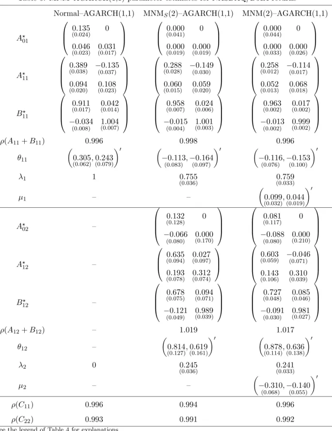
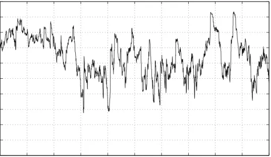
Another potentially relevant issue for financial applications is whether there are strik-ing differences between the regime–specific correlation coefficients. Figure 1 displays the component–specific conditional correlations implied by the MNM(2)–GARCH(1,1) model.8

The upper panel plots the conditional correlations in the positive–mean/low–volatility compo-nent, and the lower panel those in the negative–mean/high–volatility component. Most of the time, the correlation coefficient in the low–volatility regime is considerably smaller than that in the high–volatility regime, with the regimes’ averages being 0.643 and 0.813, respectively.

7_{Admittedly, the interpretation of ρ(A}

12+B12) as a persistence measure is a little awkward whenρ(A12+

B12)>1. 8

It is clear that such a pattern can have significant implications for portfolio diversification, which will be a topic of future investigation. To tackle this task systematically, however, it may be more convenient to specify the dynamics in the correlation matrix directly, by using, for example, structures as proposed in Engle (2002), Tse and Tsui (2002), and, more recently, Pelletier (2006).

As the largest eigenvalue of the matrix C22, reported in the bottom row of Tables 4 and

5, is below unity for all models, we can compute the theoretical auto– and cross–correlations implied by the fitted processes. As noted, for example, by He and Ter¨asvirta (2004), such calculations can help to assess whether a fitted model is capable of reproducing some of the dynamic properties of the data being investigated.

The auto– and cross–correlations are shown in Figures 2–9, along with their empirical counterparts. As expected, the mixture models mimic the empirical shapes much better than the single–component models, although the fit is not “optimal”. A somewhat more surprising observation is the fact that the AGARCH specifications capture the observed auto-and cross-correlation structure less well than their GARCH counterparts. In particular, the AGARCH–implied auto– and cross–correlations tend to be somewhat smaller than the corre-sponding GARCH quantities. At first sight, and in view of Example 2 in Appendix C.2, this is somewhat surprising, as it is shown there, that, at least for the special case of the univariate QGARCH(1,1), the autocorrelations areincreasing in θ2_{. However, this result is true only if}

all other parameters of the model are held constant, and this is obviously not the case for the estimates reported in Tables 4 and 5. Nevertheless, these findings may indicate that, within the asymmetric GARCH structure adopted in (6), there is a trade–off between reproducing the correlation structure of the squares and capturing the asymmetric response of volatility to good and bad news. A possible consequence of this is to investigate other parameterizations of the leverage effect, such as that of Glosten, Jagannathan, and Runkle (1993) which has been used for multivariate GARCH models by Hansson and H¨ordahl (1998) and Kroner and Ng (1998).

4

Conclusions

In this paper, we have generalized the normal mixture GARCH model introduced in Haas, Mittnik, and Paolella (2004a) to the multivariate framework. For the vech representation of the multivariate GARCH process, conditions for covariance stationarity and the existence of the fourth moment were presented, along with expressions for the autocorrelation function of the squares.

19900 1991 1992 1993 1994 1995 1996 1997 1998 1999 2000 0.1 0.2 0.3 0.4 0.5 0.6 0.7 0.8 0.9 1

Conditional correlations in the low−volatility component

time correlation 19900 1991 1992 1993 1994 1995 1996 1997 1998 1999 2000 0.1 0.2 0.3 0.4 0.5 0.6 0.7 0.8 0.9 1

Conditional correlations in the high−volatility component

time

correlation

Figure 1: Shown are the implied component–specific correlations of the MNM(2)–GARCH(1,1) model, fitted to the NASDAQ/DJIA returns. The upper panel shows the conditional correla-tions in the low–volatility component, those in the high–volatility component are depicted in the lower panel.

0 50 100 150 −0.1 −0.05 0 0.05 0.1 0.15 0.2 0.25 0.3 NASDAQ: Normal−GARCH(1,1) lag autocorrelation 0 50 100 150 −0.1 −0.05 0 0.05 0.1 0.15 0.2 0.25 0.3 NASDAQ: MNM S(2)−GARCH(1,1) lag autocorrelation 0 50 100 150 −0.1 −0.05 0 0.05 0.1 0.15 0.2 0.25 0.3 NASDAQ: MNM(2)−GARCH(1,1) lag autocorrelation

Figure 2: Shown are the empirical autocorrelations (vertical bars) of the squared (filtered) NASDAQ returns, as well as their theoretical counterparts (solid lines), as implied by the fitted Normal–GARCH(1,1) (top panel), MNMS(2)–GARCH(1,1) (middle panel), and MNM(2)–

GARCH(1,1) (bottom panel) models. The usual 95% asymptotic confidence intervals (dashed lines) associated with a white noise process with finite second moment are also included.

0 50 100 150 −0.1 −0.05 0 0.05 0.1 0.15 0.2 0.25 0.3 NASDAQ: Normal−AGARCH(1,1) lag autocorrelation 0 50 100 150 −0.1 −0.05 0 0.05 0.1 0.15 0.2 0.25 0.3 NASDAQ: MNM S(2)−AGARCH(1,1) lag autocorrelation 0 50 100 150 −0.1 −0.05 0 0.05 0.1 0.15 0.2 0.25 0.3 NASDAQ: MNM(2)−AGARCH(1,1) lag autocorrelation

Figure 3: Shown are the empirical autocorrelations (vertical bars) of the squared (filtered) NASDAQ returns, as well as their theoretical counterparts (solid lines), as implied by the fitted Normal–AGARCH(1,1) (top panel), MNMS(2)–AGARCH(1,1) (middle panel), and MNM(2)–

AGARCH(1,1) (bottom panel) models. The usual 95% asymptotic confidence intervals (dashed lines) associated with a white noise process with finite second moment are also included.

0 50 100 150 −0.1 −0.05 0 0.05 0.1 0.15 0.2 0.25 DJIA: Normal−GARCH(1,1) lag autocorrelation 0 50 100 150 −0.1 −0.05 0 0.05 0.1 0.15 0.2 0.25 DJIA: MNM S(2)−GARCH(1,1) lag autocorrelation 0 50 100 150 −0.1 −0.05 0 0.05 0.1 0.15 0.2 0.25 DJIA: MNM(2)−GARCH(1,1) lag autocorrelation

Figure 4: Shown are the empirical autocorrelations (vertical bars) of the squared (filtered) DJIA returns, as well as their theoretical counterparts (solid lines), as implied by the fitted Normal–GARCH(1,1) (top panel), MNMS(2)–GARCH(1,1) (middle panel), and MNM(2)–

GARCH(1,1) (bottom panel) models. The usual 95% asymptotic confidence intervals (dashed lines) associated with a white noise process with finite second moment are also included.

0 50 100 150 −0.1 −0.05 0 0.05 0.1 0.15 0.2 0.25 DJIA: Normal−AGARCH(1,1) lag autocorrelation 0 50 100 150 −0.1 −0.05 0 0.05 0.1 0.15 0.2 0.25 DJIA: MNM S(2)−AGARCH(1,1) lag autocorrelation 0 50 100 150 −0.1 −0.05 0 0.05 0.1 0.15 0.2 0.25 DJIA: MNM(2)−AGARCH(1,1) lag autocorrelation

Figure 5: Shown are the empirical autocorrelations (vertical bars) of the squared (filtered) DJIA returns, as well as their theoretical counterparts (solid lines), as implied by the fitted Normal–AGARCH(1,1) (top panel), MNMS(2)–AGARCH(1,1) (middle panel), and MNM(2)–

AGARCH(1,1) (bottom panel) models. The usual 95% asymptotic confidence intervals (dashed lines) associated with a white noise process with finite second moment are also included.

0 50 100 150 −0.1 −0.05 0 0.05 0.1 0.15 0.2 0.25

NASDAQ/lagged DJIA: Normal−GARCH(1,1)

lag cross−correlation 0 50 100 150 −0.1 −0.05 0 0.05 0.1 0.15 0.2 0.25 NASDAQ/lagged DJIA: MNM S(2)−GARCH(1,1) lag cross−correlation 0 50 100 150 −0.1 −0.05 0 0.05 0.1 0.15 0.2 0.25

NASDAQ/lagged DJIA: MNM(2)−GARCH(1,1)

lag

cross−correlation

Figure 6: Shown are the empirical cross–correlations (vertical bars) of the (filtered) NASDAQ and DJIA returns, i.e., Corr(r₁2_t, r₂2_,t−τ),τ = 1, . . . ,150, wherer1tandr2tare the time–treturns

of the NASDAQ and the DJIA, respectively. The solid lines represent the corresponding theoretical quantities, as implied by the fitted Normal–GARCH(1,1) (top panel), MNMS(2)–

GARCH(1,1) (middle panel), and MNM(2)–GARCH(1,1) (bottom panel) models. The usual 95% asymptotic confidence intervals (dashed lines) associated with a white noise process with finite second moment are also included.

0 50 100 150 −0.1 −0.05 0 0.05 0.1 0.15 0.2 0.25

NASDAQ/lagged DJIA: Normal−AGARCH(1,1)

lag cross−correlation 0 50 100 150 −0.1 −0.05 0 0.05 0.1 0.15 0.2 0.25 NASDAQ/lagged DJIA: MNM S(2)−AGARCH(1,1) lag cross−correlation 0 50 100 150 −0.1 −0.05 0 0.05 0.1 0.15 0.2 0.25

NASDAQ/lagged DJIA: MNM(2)−AGARCH(1,1)

lag

cross−correlation

Figure 7: Shown are the empirical cross–correlations (vertical bars) of the (filtered) NASDAQ and DJIA returns, i.e., Corr(r₁2_t, r₂2_,t−τ),τ = 1, . . . ,150, wherer1tandr2tare the time–treturns

of the NASDAQ and the DJIA, respectively. The solid lines represent the corresponding theoretical quantities, as implied by the fitted Normal–AGARCH(1,1) (top panel), MNMS(2)–

AGARCH(1,1) (middle panel), and MNM(2)–AGARCH(1,1) (bottom panel) models. The usual 95% asymptotic confidence intervals (dashed lines) associated with a white noise process with finite second moment are also included.

0 50 100 150 −0.1 −0.05 0 0.05 0.1 0.15 0.2 0.25

DJIA/lagged NASDAQ: Normal−GARCH(1,1)

lag cross−correlation 0 50 100 150 −0.1 −0.05 0 0.05 0.1 0.15 0.2 0.25 DJIA/lagged NASDAQ: MNM S(2)−GARCH(1,1) lag cross−correlation 0 50 100 150 −0.1 −0.05 0 0.05 0.1 0.15 0.2 0.25

DJIA/lagged NASDAQ: MNM(2)−GARCH(1,1)

lag

cross−correlation

Figure 8: Shown are the empirical cross–correlations (vertical bars) of the (filtered) NASDAQ and DJIA returns, i.e., Corr(r₁2_,t−τ, r2_2t),τ = 1, . . . ,150, wherer1tandr2tare the time–treturns

of the NASDAQ and the DJIA, respectively. The solid lines represent the corresponding theoretical quantities, as implied by the fitted Normal–GARCH(1,1) (top panel), MNMS(2)–

GARCH(1,1) (middle panel), and MNM(2)–GARCH(1,1) (bottom panel) models. The usual 95% asymptotic confidence intervals (dashed lines) associated with a white noise process with finite second moment are also included.

0 50 100 150 −0.1 −0.05 0 0.05 0.1 0.15 0.2 0.25

DJIA/lagged NASDAQ: Normal−AGARCH(1,1)

lag cross−correlation 0 50 100 150 −0.1 −0.05 0 0.05 0.1 0.15 0.2 0.25 DJIA/lagged NASDAQ: MNM S(2)−AGARCH(1,1) lag cross−correlation 0 50 100 150 −0.1 −0.05 0 0.05 0.1 0.15 0.2 0.25

DJIA/lagged NASDAQ: MNM(2)−AGARCH(1,1)

lag

cross−correlation

Figure 9: Shown are the empirical cross–correlations (vertical bars) of the (filtered) NASDAQ and DJIA returns, i.e., Corr(r₁2_,t−τ, r2_2t),τ = 1, . . . ,150, wherer1tandr2tare the time–treturns

of the NASDAQ and the DJIA, respectively. The solid lines represent the corresponding theoretical quantities, as implied by the fitted Normal–AGARCH(1,1) (top panel), MNMS(2)–

AGARCH(1,1) (middle panel), and MNM(2)–AGARCH(1,1) (bottom panel) models. The usual 95% asymptotic confidence intervals (dashed lines) associated with a white noise process with finite second moment are also included.

An application to daily returns of the NASDAQ and Dow Jones indices shows that the model captures interesting and relevant properties of the bivariate volatility process, such as regime–dependent leverage effects and conditional correlations. In view of these findings, it would be desirable to consider extensions of the model which allow for conditional forecasts of the next period’s regime, which is not possible within the iid multinomial mixture approach adopted here.

A well–known disadvantage of the BEKK representation of the multivariate GARCH model is its large number of parameters, which renders estimation quite difficult when the dimension of the return series is larger than three or four. While this is true for standard GARCH models, this curse of dimensionality is even more burdensome in the mixture framework, as we have as many covariance matrices as mixture components. Thus, future research will concentrate on developing more parsimonious parameterizations for the component–specific covariance matrices. Factor structures as proposed in Alexander and Chibumba (1997), and Alexander (2001, 2002), as well as the dynamic conditional correlation models of Engle (2002), and Tse and Tsui (2002), are natural starting points to deal with this issue.

Another important topic of further research is the empirical comparison of the mixture GARCH process with other flexible multivariate GARCH models, such as those of Bauwens and Laurent (2005), and Aas, Haff, and Dimakos (2006), who employ a multivariate skewedt

and the multivariate normal inverse Gaussian distribution, respectively.

Appendix

In the Appendix, we derive the conditions for the moments of the MNM–GARCH model. We also provide expressions for these moments and the autocorrelation structure of the process.

A

Notation

To conveniently write down the unconditional moments of the multivariate normal mixture GARCH model, use of several patterned matrices is rather advantageous, and we define them here. A detailed discussion of (as well as explicit expressions for) these matrices can be found in Magnus (1988).9 The first of these matrices is thecommutation matrix,Kmn, which is the

mn×mnmatrix with the property thatKmnvec(A) = vec(A0) for everym×nmatrixA. We

will use the fact that the commutation matrix allows us to transform the vec of a Kronecker 9

Chapter 1 of Magnus and Neudecker (1999) also provides useful information, as do the appendices in Hafner (2003) and L¨utkepohl (2005).

product into the kronecker product of the vecs (Magnus, 1988, Theorem 3.6). More precisely, for anm×nmatrixA and anp×q matrixB, it is true that

vec(A⊗B) = (In⊗Kqm⊗Ip)(vecA⊗vecB). (A.1)

The elimination matrix, Ln, is the n(n+ 1)/2×n2 matrix that takes away the redundant

elements of a symmetric n×n matrix, i.e., for every n×n matrix A, we have Lnvec(A) =

vech(A). In contrast, the duplication matrix, Dn, is the n2 ×n(n+ 1)/2 matrix with the

property that Dnvech(A) = vec(A) for every symmetric n×n matrixA. Its Moore–Penrose

inverse,D+_n, is given by D_n+= (D_n0Dn)−1D0n(Magnus, 1988, Theorem 4.1).

To compactify the expressions for the moments of our model, we will also made extensive use of the matrix Nn = (In2 +K_nn)/2, which is discussed in Section 3.10 of Magnus (1988), and which has the property that, for everyn×n matrixA,

2Nnvec(A) = vec(A+A0). (A.2)

Note that the matrixD+_n has a similar property. Namely, because of D+_n =LnNn (Magnus,

1988, p. 80), we have

2D_n+vec(A) = vech(A+A0). (A.3)

B

The Third and Fourth Moments of an Asymmetric

Multi-variate Normal Mixture Distribution

In this Appendix, we provide convenient expressions for the expectations of vec[vech(xx0_)x0_]

and vec[vech(xx0)vech(xx0)0], when x has a multivariate normal mixture distribution with (possibly) nonzero means, as defined in (1) and (2). These expressions will be useful for computing the unconditional moments of the multivariate mixed normal GARCH process in Appendices C and D.

To derive the expressions given in this Appendix, we draw on results of Magnus and Neudecker (1979), Balestra and Holly (1990), and Hafner (2003). We state the central results as Lemmas 2–4 for the third, and Lemmas 5–8 for the fourth moment. Details of the derivations are presented only for the third moment, because those for the fourth moment are similar.10

B.1 The Third Moment

To find an expression for vec[vech(xx0_)x0_{], which is needed due to the inclusion of the leverage}

terms, we make use of a formula of Balestra and Holly (1990) which we state as Lemma 2. 10

Lemma 2 (Balestra and Holly, 1990) For anM–dimensional random vectorx, which is nor-mally distributed with meanµ and covariance matrix H, we have

E[(x⊗x)x0] =vec(H)µ0+ 2NM(µ⊗H) + (µ⊗µ)µ0. (B.4)

We are interested in E{vec[vech(xx0_)x0_{]} as a linear function in h, where h = vech(H).}

Such an expression is provided next.

Lemma 3 For anM–dimensional random vector x, which is normally distributed with mean

µand covariance matrix H, we have

E{vec[vech(xx0)x0]}= (IM ⊗LM)[ ˜GM(µ⊗DM)h+µ⊗µ⊗µ], (B.5)

where h=vech(H), and

˜

GM =IM3+ 2(I_M ⊗N_M)(K_{M M}⊗I_M). (B.6)

Proof. By Lemma 2, and using vec(ABC) = (C0_{⊗A)vec(B), we have}

E{vec[vech(xx0)x0]} = E{vec[LMvec(xx0)x0]}= (IM ⊗LM)E{vec[(x⊗x)x0]}

= (IM ⊗LM)vec[vec(H)µ0+ 2NM(µ⊗H) + (µ⊗µ)µ0].

Furthermore, vec[2NM(µ⊗H)] = 2(IM ⊗NM)vec(µ⊗H), and (A.1) implies that vec(µ⊗

H) = (KM M ⊗IM)(µ⊗vec(H)). Finally, as y⊗x = vec(xy0) for vectors x and y, we have

µ⊗vec(H) = vec[vec(H)µ0] = vec(DMhµ0) = (µ⊗DM)h, and thus (B.5).

Next, we consider the case of a normal mixture distribution.

Lemma 4 Assume that x ∼MNM(λ1, . . . , λk, µ1, . . . , µk, H1, . . . , Hk). Let λ= (λ1, . . . , λk)0,

Λ =diag(λ); hj =vech(Hj), j = 1, . . . , k; h= (h01, . . . , h0k)0; Υ = (µ1, . . . , µk); µ=vec(Υ) =

(µ0

1, . . . , µ0k)0;µ˜j =vech(µjµ0j),j = 1, . . . , k; Υ = (˜˜ µ1, . . . ,µ˜k); and˜µ=vec( ˜Υ) = (˜µ01, . . . ,µ˜0k)0.

Then,

E{vec[vech(xx0)x0]} (B.7)

= (IM ⊗LM) ˜GM(ΥΛ⊗DM)h+ (IM ⊗vec(Λ)0⊗IN)(KM k⊗IkN)vec(˜µµ0),

where N =M(M + 1)/2, and G˜M is defined in (B.6).

Proof. Lemma 4 follows from the fact that the third moment of the mixture is just the weighted average of the component–specific moments as given in (B.5), i.e., forxmixed normal as defined in Lemma 4, we have

E{vec[vech(xx0)x0]}= (IM ⊗LM)    ˜ GM k X j=1 λj(µj⊗DM)hj+ k X j=1 λj(µj⊗µj⊗µj)    . (B.8)

Letej be thejth unit vector in Rk. Then, for the first sum on the right–hand side of (B.8), we have that k X j=1 λj(µj ⊗DM)hj =    k X j=1 λj(e0j⊗µj⊗DM)    h=      k X j=1 λjµje0j  ⊗D_M    h = (ΥΛ⊗DM)h, (B.9)

where, in the last equation of the first line in (B.9), we have used that y0_{⊗x =xy}0_{. For the}

second sum on the right–hand side of (B.8), we find

X j λj(µj ⊗µj⊗µj) = X j λjvec[(µj⊗µj)µ0j] = (IM⊗DM) X j λjvec(˜µjµ0j) (B.10) = (IM ⊗DM) X j λjvec[(e0j⊗IN)(˜µµ0)(ej⊗IM)] = (IM ⊗DM) X j λj(e0j⊗IM ⊗e0j⊗IN)vec(˜µµ0) = (IM ⊗DM) X j λj(IM⊗e0j ⊗e0j⊗IN)(KM k⊗IkN)vec(˜µµ0) = (IM ⊗DM) X j λj(IM⊗vec(eje0j)0⊗IN)(KM k⊗IkN)vec(˜µµ0) = (IM ⊗DM)(IM ⊗vec(Λ)0⊗IN)(KM k⊗IkN)vec(˜µµ0),

where we have used the identity (A⊗b0)Knp =b0⊗A form×nmatrixA and p×1 vector b

(Magnus, 1988, p. 36). Finally, because (A⊗B)(C⊗D) = (AC)⊗(BD) ifAC and BDexist, we have (IM ⊗LM)(IM ⊗DM) = (IM ⊗LMDM), and, by Theorem 5.5 of Magnus (1988),

LMDM =IN,N =M(M+ 1)/2, so we get (B.7).

B.2 The Fourth Moment

For the fourth moment, we build on results of Magnus and Neudecker (1979) and Hafner (2003) which we state as Lemmas 5 and 6, respectively.

Lemma 5 (Magnus and Neudecker, 1979, Theorem 4.3) For anM–dimensional random vec-torx, which is normally distributed with mean µ and covariance matrixH, we have11

E[(x⊗x)(x⊗x)0] = 2DMD_M+(H⊗H) +vec(H)vec(H)0 (B.11)

+2DMD_M+(H⊗µµ0+µµ0⊗H)

+vec(H)vec(µµ0)0+vec(µµ0)vec(H)0+vec(µµ0)vec(µµ0)0.

11_{Magnus and Neudecker (1979) state the result in terms of the matrix N}

n defined in Appendix A. In fact,

by Theorem 4.2 of Magnus (1988), we haveNn=DnD+n. Here, the representation in terms of DnD+n is

For the result in Lemma 5 and generalizations, see also Magnus (1988, Ch. 10) and Ghazal and Neudecker (2000).

We are interested in E[vech(xx0)vech(xx0)0]. Using the identity vec(xx0) = x⊗x and the definition of the elimination matrixLM, this can be written asLME[(x⊗x)(x⊗x)0]L0M, which

is a simple transformation of (B.11). The case of a normal distribution with zero mean was considered by Hafner (2003).12

Lemma 6 (Hafner, 2003, Theorem 1) For an M–dimensional normally distributed random vector x with zero mean and covariance matrix H, we have

vec{E[vech(xx0)vech(xx0)0]}=GMvec(hh0), (B.12)

where h=vech(H), and

GM = 2(LM ⊗DM+)(IM⊗KM M⊗IM)(DM ⊗DM) +IN2, (B.13)

andN :=M(M+ 1)/2 is the number of independent elements in H.

Our first step is to generalize (B.12) to the case of nonzero means, i.e., to consider the terms in the second and third line of (B.11).

Lemma 7 For an M–dimensional normally distributed random vector x with mean µ and covariance matrixH, we have

vec{E[vech(xx0)vech(xx0)0]}=GMvec(hh0) + 2GMNN(˜µ⊗IN)h+vec(˜µµ˜0), (B.14)

where GM is defined in (B.13), h=vech(H), µ˜=vech(µµ0), and N =M(M+ 1)/2.

The proof of Lemma 7 can be carried out along similar lines as the proof of Theorem 1 in Hafner (2003). The case of a multivariate normal mixture distribution is considered next. We make use of the notation introduced in Lemma 4.

Lemma 8 Assume thatx∼MNM(λ1, . . . , λk, µ1, . . . , µk, H1, . . . , Hk). Then,

vec{E[vech(xx0)vech(xx0)0]} (B.15)

=GM(IN ⊗vec(Λ)0⊗IN)(KN k⊗IkN)vec(hh0) + 2GMNN( ˜ΥΛ⊗IN)h

+(IN ⊗vec(Λ)0⊗IN)(KN k⊗IkN)vec(˜µµ˜0).

12

Actually, Hafner (2003) considered the more general class of spherical distributions which includes the normal as a special case.

Lemma 8 is obtained by combining the results of Lemma 7 with the fact that the fourth moment of the mixture is just the weighted average of the component–specific moments as given in (B.14), quite similar to equation (B.8) for the third moment, and by using arguments similar to those in the derivation of Lemma 4. For example, to show that

k

X

j=1

λjvec(hjh0j) = (IN ⊗vec(Λ)0⊗IN)(KN k⊗IN k)vec(hh0), (B.16)

we essentially repeat the argument in (B.10).

C

The Moments of the MNM(k)–AGARCH(1,1) Model

In this Appendix, we use the results of Appendix B to derive the unconditional second and fourth moments of the asymmetric multivariate mixed normal GARCH(1,1) model as given in equation (11), as well as the conditions for their existence. Using the results of Balestra and Holly (1990), higher–order moments could in principle also be derived, but the resulting expressions become unmanageable even for the central normal distribution, as the number of terms to be evaluated is explosive as the order increases. Thus, in view of the fact that such higher moments are of minor interest in applications, we concentrate on the second and the fourth moment.13

C.1 Moment Conditions

We will use the notation introduced in Section 2 and Lemmas 4 and 8. Also, as defined in (12),ρ(A) denotes the largest eigenvalue in modulus of a square matrix A.

Define Wt = (h0t,vec(hth0t)0)0, and consider the expectation of Wt at time t− 2, i.e.,

E(Wt|Ψt−2). Clearly E(ηt−1|Ψt−2) = (λ0⊗IN)(ht−1+ ˜µ), so that14

E(ht|Ψt−2) = ˜A0+A1(λ0⊗IN)˜µ+ (λ⊗A1+B1)ht−1.

The conditional expectation of vec(hth0t) can be greatly simplified by extensively using the

matrixNn, and in particular its basic property (A.2). In addition, we will frequently use the

identities vec(xy0) =y⊗x and vec(ABC) = (C0⊗A)vec(B). Thus,

vec(hth0t) = A˜0⊗A˜0+ 2NkNvec[ ˜A0(ηt0−1A10 +h0t−1B10)] + 2NkNvec(A1ηt−1h0t−1B01)

+(A1⊗A1)vec(ηt−1ηt0−1) + (B1⊗B1)vec(ht−1h0t−1)

+vec(Θ1t−10t−1Θ01)−2NkNvec[( ˜A0+A1ηt−1+B1ht−1)0t−1Θ01]. (C.17) 13

For the univariate case, a condition for the existence of arbitrary integer even moments in given in Haas, Mittnik and Paolella (2004a).

14

Let us evaluate the conditional expectations of the components of (C.17). Observe that E{vec( ˜A0ηt0−1A10)|Ψt−2} = vec{A˜0(h0t−1+ ˜µ0)(λ⊗IN)A01} = [A1(λ0⊗IN)⊗A˜0](ht−1+ ˜µ) = (λ0⊗A1⊗A˜0)(ht−1+ ˜µ), and E[vec(A1ηt−1h0t−1B10)|Ψt−2] = vec[A1(λ0⊗IN)(ht−1+ ˜µ)h0t−1B10] = (B1⊗λ0⊗A1)vec(ht−1h0t−1) + (B1⊗λ0⊗A1)vec(˜µh0t−1) = (B1⊗λ0⊗A1)vec(ht−1h0t−1) + (B1⊗λ0⊗A1)(IkN ⊗µ˜)ht−1 = (B1⊗λ0⊗A1)vec(ht−1h0t−1) + [B1⊗(λ0⊗A1)˜µ]ht−1.

The expectation of (A1⊗A1)vec(ηt−1ηt0−1), given Ψt−2, follows from Lemma 8. It remains

to consider those terms of (C.17) which involve t−1. First, note that E(ht−10t−1|Ψt−2) =

ht−1E(0t−1|Ψt−2) = 0. Thus, we have two nonzero terms. The first is

E[vec(Θ1t−10t−1Θ01)|Ψt−2] = (Θ1⊗Θ1)DM(λ0⊗IN)(ht−1+ ˜µ),

and the second, using Lemma 4,

E[vec(A1ηt−10t−1Θ01)|Ψt−2] = (Θ1⊗A1) h (IM ⊗LM) ˜GM(ΥΛ⊗DM)ht−1 +(IM ⊗vec(Λ)0⊗IN)(KM k⊗IkN)vec(˜µµ0) . Next, define d=   d1 d2  , C=   C11 0kN×kN C21 C22  , where d1 = A˜0+A1(λ0⊗IN)˜µ d2 = A˜0⊗A˜0+ 2NkN(λ0⊗A1⊗A˜0)˜µ+ (A1⊗A1)(IN⊗vec(Λ)0⊗IN)(KN k⊗IkN)vec(˜µµ˜0) +(Θ1⊗Θ1)DM(λ0⊗IN)˜µ−2NkN(Θ1⊗A1)(IM ⊗vec(Λ)0⊗IN)(KM k⊗IkN)vec(˜µµ0), C11 = λ0⊗A1+B1, C21 = 2NkN(λ0⊗A1+B1)⊗A˜0+ 2NkN[B1⊗(λ0⊗A1)˜µ] + 2(A1⊗A1)GMNN( ˜ΥΛ⊗IN) +(Θ1⊗Θ1)DM(λ0⊗IN)−2NkN(Θ1⊗A1)(IM ⊗LM) ˜GM(ΥΛ⊗DM), C22 = (A1⊗A1)GM(IN ⊗vec(Λ)0⊗IN)(KN k⊗IkN) + 2NkN(B1⊗λ0⊗A1) +B1⊗B1.

From the preceding analysis it is clear that E(Wt|Ψt−2) =d+CWt−1, and, by iteration, E(Wt|Ψt−τ−1) = τ−1 X i=0 Cid+CτWt−τ. (C.18)

From the block–triangular structure ofC, we have, from (C.18), that E(ht|Ψt−τ−1) =

τ−1

X

i=0

C₁₁i d1+C11τ ht−τ. (C.19)

Thus, as we have assumed that the process starts indefinitely far in the past with finite fourth moments, the unconditional expectation E(ht) exists and is given by the limit as τ → ∞, i.e.,

E(ht) = lim τ→∞E(ht|Ψt−τ−1) = ∞ X i=0 C₁₁i d1 = (IkN −C11)−1d1

if and only ifρ(C11)<1, as stated in (13). By the same line of reasoning, E(Wt) exists and is

given by (I−C)−1dif and only if E(ht) exists and ρ(C22)<1, as claimed in (14).

Example 1 Note that the expressions for the elements of d and C defined above simplify considerably if all mixture components have zero means, which may be appropriate when the (conditional) distribution of the returns under study exhibits leptokurtosis but no asymmetries. In particular, in this case the only extra term due to the leverage effects is(Θ1⊗Θ1)DM(λ0⊗IN)

in the lower left block of C, i.e.,C21. Moreover, in the univariate, single–component case we

get the QGARCH(1,1) model of Sentana (1995); and the unconditional fourth moment, in obvious notation, is E(η_t2) =E(4_t) = 3α0[α0(1 +α1+β1) +θ 2 1] (1−α1−β1)(1−3α12−2α1β1−β21) , (C.20)

which was given by Sentana (1995). This differs from the fourth moment of the standard GARCH(1,1) model of Bollerslev (1986) only by the extra θ₁2 in the numerator of (C.20), which shows that the QGARCH(1,1) model has a greater fourth moment than its standard GARCH(1,1) counterpart. The variance, however, is E(2_t) = α0/(1−α1 −β1), as in the

standard GARCH(1,1), and the kurtosis is given by

κ= E( 4 t) E2(2 t) = 31−(α1+β1) 2_{+ (1−α} 1−β1)θ2/α0 1−3α2₁−2α1β1−β₁2 = 31−(α1+β1) 2_+θ2_/E(2 t) 1−3α2₁−2α1β1−β₁2 ,

which depends on the scale parameterα0. Due to the factorθ2/E(2t), the unconditional kurtosis

of the QGARCH(1,1) model exceeds that of the standard GARCH(1,1) process. However, as stressed by Carnero, Pe˜na, and Ruiz (2004), in applications, θ2 _{is usually small relative to}

C.2 Autocovariance Function of the Squares

To find the autocovariance matrices, i.e., Γτ = E(ηtη0t−τ)−E(ηt)E(ηt)0, we first note that

(C.19) in Appendix C.1 implies E(ht|Ψt−τ) = τ−2 X i=0 C₁₁i di+C11τ−1ht−τ+1= E(ht) +C11τ−1[ht−τ+1−E(ht)]. Hence, E(ηtη0t−τ) = E[E(ηt|Ψt−τ)ηt0−τ] = E{(λ0⊗IN)[E(ht|Ψt−τ) + ˜µ]ηt0−τ} = (λ0⊗IN)E{[E(ht) + ˜µ+C11τ−1(ht−τ+1−E(ht))]η0t−τ} = E(ηt)E(ηt)0+ (λ0⊗IN)C11τ−1E n [ ˜A0+A1ηt−τ−Θ1t−τ+B1ht−τ−E(ht)]η0t−τ o .

Thus we have (15) with

Q= En[ ˜A0+A1ηt−Θ1t+B1ht−E(ht)]ηt0

o

. (C.21)

Example 2 For Sentana’s (1995) univariate QGARCH(1,1) process considered in Example 1, tedious calculations show that the autocorrelation function of the squares is given by

rτ =      2α0α1(1−α1β1−β21)+(3α1+β1)(1−α1−β1)θ2 2α0(1−2α1β1−β12)+3(1−α1−β1)θ2 τ = 1 (α1+β1)rτ−1 τ >1. (C.22)

Thus, the decay pattern of the ACF is equal to that of the standard GARCH(1,1) process, as already noted by Sentana (1995). However, for given values ofα0,α1, andβ1, the ACF of the

QGARCH(1,1) process is always larger than that of the GARCH(1,1), and is increasing inθ2: It is straightforward to see that∂rτ/∂θ2 >0is equivalent toα1(1−α1β1−β12)(3α1+β1)−1<(1−

2α1β1−β12)/3, and simple manipulations reveal that this is equivalent to3α21+ 2α1β1+β12 <1,

which is just the condition for the existence of the fourth moment, and, thus, the ACF of2

t.

D

Moments of the MNM(

k

)–GARCH(

p, q

) process

In this Appendix, we indicate how the moments of the MNM(k)–GARCH(p, q) model may be computed for higher–order GARCH models, i.e., with p and/or q larger than 1. We keep the discussion short, because in most applications GARCH(1,1) rather than GARCH(p, q) will suffice, and the properties of the GARCH(1,1) case have been developed in detail in the preceding appendix. Moreover, in order to avoid clutter, we shall assume that all the

components have zero means, i.e., in (5), µj = 0, j= 1, . . . , k, and that there are no leverage

effects, i.e., in (6),θij = 0,i= 1, . . . , q,j= 1, . . . , k.

Recently, using the ARMA representation of a GARCH model, Zadrozny (2005) employed a state–space representation of the univariate GARCH(p, q) process to derive a condition for the existence of its fourth moment.15 We use a similar approach to find a condition for the existence of the unconditional fourth–moment matrix of the multivariate mixed normal GARCH model. However, we use a different representation than Zadrozny (2005). Although the representation we use is less parsimonious, it is preferred in present context because, in addition to providing a condition and an expression for the fourth moment, it allows for the computation of the autocorrelation matrices of the process. Clearly, the results presented here also apply to the single–component case, i.e., the standard GARCH(p, q) model in vech form, the fourth–moment structure of which has been investigated by Hafner (2003). However, Hafner’s (2003) analysis is based on the MA(∞) representation of the process, which makes the application of the results less convenient. A brief comparison of Hafner’s (2003) analysis with our approach is provided at the end of this Appendix. A condition for the existence of the fourth moment in single–component multivariate GARCH(p, q) models has also been derived by Comte and Liebermann (2000).16 _{Their condition involves a matrix which is composed of}

2q terms, where q is the ARCH order. Forq = 1, this matrix coincides with the matrix Z in Theorem 3 of Hafner (2003). However, Comte and Liebermann (2000) do not consider how to compute the autocovariances from their approach.

To write the model in VARMA form, define ¯h= E(ηt|ψt−1) = (λ0⊗IN)ht, andut=ηt−¯ht,

so that{ut}is a white noise process (uncorrelated but not independent).17 Then we can write

the MNM–GARCH(p, q) process as a VARMA(r, v) model for ht, i.e.,

ht=A0+ r X i=1 Ciht−i+ v X i=1 Aiut−i, (D.23)

where r = max{p, q}, v = max{q,2}, Ci =λ0⊗Ai+Bi, Ai = 0, for i > q, and Bi = 0, for

i > p. To put the MNM–GARCH(p, q) model in VAR(1) form, we adopt a slightly modified form of the VAR(1) representation of a VARMA model discussed in L¨utkepohl (2005, p. 426).

15

Papers dealing with the fourth–moment structure of the univariate GARCH(p, q) model include Chen and An (1998), He and Ter¨asvirta (1999), Karanasos (1999), Ling (1999), Davidson (2002, Section 2.3), and Ling and McAleer (2002). There also exist results for other multivariate GARCH models than the vech model. For example, moment conditions for Jeantheau’s (1998) generalization of Bollerslev’s (1990) constant conditional correlation model are derived in Ling and McAleer (2003) and He and Ter¨asvirta (2004).

16_{Computation of the fourth moment in the bivariate case was also considered by Nijman and Sentana (1996).} 17

That is, we define Xt =               ht .. . ht−r+1 ut−1 .. . ut−v+1               , A˜0=   A0 0_{N{k(r−1)+(v−1)}×1}  , Z=        A1 0_{N k(r−1)×N} IN 0_N(v−2)×N        , H =   H11 H12 H21 H22  , where H₁₁=   C1 · · · Cr−1 Cr I_kN(r−1) 0_{kN(r−1)×kN}  , H12 =   A2 · · · Av 0_{kN(r−1)×N(v−1)}  , H₂₂=   0N×N(v−2) 0N×N I_N(v−2) 0_N(v−2)×N  , (D.24)

andH21is a N(v−1)×kN r matrix of zeros. Thus,Xt is of dimensionN(kr+v−1). Given

the definitions in (D.24), we can write

Xt= ˜A0+HXt−1+Zut−1. (D.25)

From (D.25), we can infer that the MNG–GARCH(p, q) process is stationary if ρ(H11) <1,

or, equivalently, the roots of

det(IkN− r

X

i=1

Cizi) = 0 (D.26)

are outside the unit circle.

To find a condition for the existence of the fourth moment, i.e., of E(XtXt0), define the

matrices

I:= (IkN,0kN×N{k(r−1)+v−1}), (D.27)

so thathth0t=IXtXt0I0, and

FM :=GM(IN ⊗vec(Λ)0⊗IN)(KN k⊗IkN)−(