Supervised Learning Applied to Air Traffic Trajectory
Classification
Christabelle S. Bosson
∗USRA/NAMS, NASA Ames Research Center, Moffett Field, CA 94035, USA
Tasos Nikoleris
†USRA/NAMS, NASA Ames Research Center, Moffett Field, CA 94035, USA
Given the recent increase of interest in introducing new vehicle types and missions into the National Airspace System, a transition towards a more autonomous air traffic control system is required in order to enable and handle increased density and complexity. This paper presents an exploratory effort of the needed autonomous capabilities by exploring
supervised learning techniques in the context of aircraft trajectories. In particular, it
focuses on the application of machine learning algorithms and neural network models to a runway recognition trajectory-classification study. It investigates the applicability and effectiveness of various classifiers using datasets containing trajectory records for a month of air traffic. A feature importance and sensitivity analysis are conducted to challenge the chosen time-based datasets and the ten selected features. The study demonstrates that
classification accuracy levels of 90% and above can be reached in less than 40 seconds of
training for most machine learning classifiers when one track data point, described by the ten selected features at a particular time step, per trajectory is used as input. It also shows that neural network models can achieve similar accuracy levels but at higher training time costs.
I.
Introduction
Given the recent increase of interest in developing autonomous systems, the Air Traffic Management (ATM) research community has been busy investigating algorithms to expedite their safe integration into the National Airspace System (NAS).1, 2 A major challenge associated with this effort is to ensure that
those systems are correctly trained in order to operate with high levels of accuracy regardless of noise and uncertainty. In particular, in order to enable increased complexity and higher density operations in the NAS, future ATM autonomous tools will mainly rely on the prediction of future aircraft states. Current operations are highly complex and given recent improvements made in computational resources, machines can be trained to reason by learning concepts from large amounts of data.
Motivated by their successful application in many fields, a review of the ATM literature shows that statistical methods and machine learning techniques have been focusing on air traffic delay prediction at an aggregate level rather than on trajectories at a more detailed level. Xu et al. derived a Bayesian network approach to predict delay propagation.3 Rebollo et al. used Random Forest classification and
regression algorithms combined with air traffic network characteristics to predict air traffic delays.4 Choi
et al. implemented a machine learning model using techniques such as Decision Trees, Random Forest, AdaBoost and K-Nearest-Neighbors combined with weather data in order to predict airline delays.5
Moreover, thanks to the increase of air traffic data collection over the past few decades, data-driven methods have been derived in ATM to learn common patterns and detect anomalies. Gariel et al. applied trajectory clustering techniques to GPS radar tracks in order to identify operational aircraft behaviors and their variability.6 Gopalakrishnan et al. used graph clustering techniques to identify and characterize air
∗Research Scientist, Universities Space Research Center, NASA Ames Research Center, Moffett Field, CA 94035 AIAA
Member.
†Research Scientist, Universities Space Research Center, NASA Ames Research Center, Moffett Field, CA 94035 AIAA
Member.
traffic delay states of the NAS.7Conde Rocha Mur¸ca developed a data mining framework for air traffic flow characterization using density-based clustering algorithm to identify aircraft trajectories and ensemble-based methods to detect flight non-conforming behaviors.8 Arneson developed a methodology to compute weather
reroute predictions by applying clustering techniques to a large volume of weather data.9 Evans and Lee
applied various data mining techniques to flight plan amendment data to train a predictor of operational acceptability for airborne reroute advisories.10 Bloem and Bambos built behavioral cloning and inverse
reinforcement learning models to predict hourly Ground Delay Program implementation at Newark Liberty International and San Francisco International airports.11
In the meantime, extensive research has been performed in many fields using the deep learning paradigm which is inspired by the hierarchical structure of human perception. Deep learning was found to improve clas-sification and regression accuracy of machine learning tasks such as image clasclas-sification, speech recognition and machine translation.12–15 It has also been applied to a broad range of applications ranging from medical
research, financial stock prediction, to ground traffic flow prediction.16–18 In ATM, Kim et al. applied deep learning to flight delay prediction.19
The literature shows that there is a limited number of studies focusing on applying supervised learning techniques to classification and trajectory problems in ATM. Considering the current improvements of ma-chine learning and deep learning algorithms, it is meaningful to evaluate the applicability and effectiveness of such techniques for trajectory classification problems. This study focuses on exploring and understand-ing the application of a collection of supervised learnunderstand-ing algorithms on aircraft trajectories arrivunderstand-ing into an airport to predict the landing runways. There exist other practical applications of this study including the prediction of package delivery locations given past trajectory information and the prediction of air traffic controller intentions when providing conflict resolution maneuvers. Moreover, in the context of building an autonomous air traffic control system, the runway classification method could be used to improve the Terminal Area Automated Concept (TAAC) proposed by Erzberger et al. and Nikoleris et al. by providing a preferred runway assignment when aircraft enter the terminal airspace.20, 21 Finally, the application of
this study could be used to leverage existing pilot and controller decision support tools that help detect trajectory deviations that could potentially lead to accidents such as the recent miss runway lineup that occurred August 2017 at the San Francisco International airport (SFO).22 This present paper contributes to the field of ATM by bringing and adapting artificial learning techniques to solve a time-based trajectory classification.
The paper is organized as follows. The problem description is presented in Section II and the solution approach is described in Section III. In Section IV, the results are presented and detailed and in Section V, a summary, final remarks and extended applications of the study conclude the paper.
II.
Problem Description
This paper focuses on solving a runway recognition trajectory-classification problem. For this study, the Dallas Forth-Worth International airport (DFW) is chosen for the application.
A. Problem Formulation
The runway recognition problem is formulated as a trajectory classification study where a time series of features constituted of several data point time steps is provided as input and a classification is generated as output. Given past flown trajectory information, the goal is to predict the landing runway of each arriving aircraft.
B. Selected Features
In order to characterize trajectories, ten features are selected prior to the application of supervised learning algorithms as influencing parameters on the outcome classification. For each flight, the initial set of features contains the operating carrier, the aircraft weight category, the first closest flown-by TRACON arrival gate, the corresponding arrival gate flown-by time, and time steps of latitude, longitude, altitude, ground speed, course angle (i.e. ground track angle) and rate of climb. As a data preprocessing step, the continuous features are standardized by subtracting the mean and scaling to unit variance. Centering and scaling operations are independently computed on each feature by calculating the mean and the standard deviation on the samples in the training set. The goal here is to minimize any feature dominance and let the estimators correctly
learn from other features. For the categorical features, they are first label encoded, where each value of the categorical features is given a corresponding integer value. Then in order to prevent any misinterpretations by the different algorithms, each integer value is one-hot encoded, i.e. each value is binarized. The one-hot encoding method transforms each categorical feature withmpossible values intombinary features, with only one active. This has the benefit of not weighting a value improperly but does have the downside of adding more features to the dataset. The reader can refer to reference Pedregosa et al.23 for more information on
data preprocessing, continuous variable scaling operations and categorical feature encoding techniques. Feature selection is a complex process that enables the approximation of the underlying function between the input and the output. The goal of feature selection is to find a set of relevant features to the classification target and minimize irrelevant features that lead to greater computational cost and overfitting. It has been the subject of many studies in the field of statistics and machine learning for many years.24, 25 In this paper,
because a limited number of features was selected, no specific algorithm per say was used for feature selection. Instead, all selected features are used to train the different algorithms. However, several feature selection algorithms such as low variance removal, univariate feature selection and recursive feature elimination could be used to reduce the number of features used in the dataset.25 In the results section of this paper, a feature importance analysis is presented to determine if features dominate others and understand if a feature dimensionality reduction should be performed on the dataset in future work.
C. Airspace Details
The Dallas Forth-Worth International airport is selected for this application because of its complex runway layout. As illustrated in Figure 1, it consists of three sets of parallel runways 13L/31R and 13R/31L; 17L/35R, 17C/35C and 17R/35L; 18L/36R and 18R/36L. DFW has two primary directional traffic flows; the airport operates in South/North flow 69%/31% of the time in visual weather conditions and 56%/44% of the time in marginal weather conditions.26 For the South flow configuration, arrival flights land on 13R,
17C, 17L and 18R, and departing flights take-off from 13L, 17R and 18L. For the North flow configuration, arrival flights land on 31R, 35C, 35R and 36L, and departing flights take-off from 31L, 35L and 36R.
Most frequently, the airport operates in South flow and in 2016, there was a daily average of 529 landings and departures (data analysis using 2016 data from the Bureau Transportation System On-Time Performance database).27
Figure 1. Dallas Forth-Worth International airport layout
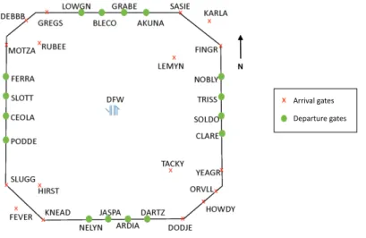
The surrounding terminal airspace (i.e. TRACON) is designated by D10, a four corner-post airspace represented in Figure 2 containing 29 airports within the DFW metroplex, for which the operations are dominated by DFW airport. Arrival flights enter D10 by using arrival gates located at the corner posts of
the TRACON boundary, whereas departure flights leave D10 using departure gates positioned on the North, South, East and West legs of the TRACON boundary. The arrival and departure gates are respectively displayed by red crosses and green dots on Figure 2. For South flow operations, the Northeast and Southwest corners are the most commonly used.
Arrival gates Departure gates
Figure 2. D10 TRACON
D. Dataset Generation
The dataset created for this study is generated from flown trajectories retrieved from Sherlock, the data warehouse that supports ATM research at NASA Ames Research Center.28 The dataset is constructed using
the month of June 2017 track data extracted in the Integrated Flight Format (IFF) for South flow Visual Flight Rules (VFR) traffic conditions at DFW. IFF is a format used by ATAC, Aviation Analysis Experts, in which flight plan and track point records are gathered from various incoming data sources merged from multiple FAA facilities. The dataset contains the final ten minutes of flight time of 20,822 arrivals operating in South flow configuration spanning 30 days of air traffic at DFW. Table 1 details the number of arrivals into DFW per runway considered in the dataset.
Table 1. Number of Arrival Flights at DFW in Dataset
Runways 13R 17C 17L 18R
Number of arrivals 712 9295 3670 7145
To illustrate the considered data, trajectories of 300 flights are randomly extracted from the dataset. Figures 3 and 4, respectively, represent 2D and 3D trajectories of the last three and last ten minutes of flight before landing. Trajectories pictured in Figure 3 are closer to the runways than trajectories pictured in Figure 4. The observable visual segregation of the flows shows that trajectories displayed in Figure 3 contain final approach trajectories, whereas in Figure 4 trajectories are extended to a larger spectrum of flight segments.
III.
Methodology - Solution Approach
In this study, we are interested in comparing different supervised learning algorithms to solve the trajec-tory classification problem described, i.e. runway recognition. Since the problem can be formulated as a time series classification, machine learning classifiers such as logistic regression, support vector machine, k-nearest neighbors, random forests and others are first investigated.29 Then, neural network solution approaches are
explored.30 For all classifiers, a 10-fold cross validation procedure is used to avoid overfitting and improve
97.20 97.15 97.10 97.05 97.00 Longitude (deg) 32.900 32.925 32.950 32.975 33.000 33.025 33.050 33.075 Latitude (deg)
2d Trajectories
17C 17L 18R 13R(a) 2d Trajectory Representation
Latitude (deg) 32.900 32.925 32.950 32.975 33.000 33.025 33.050 33.075 Longitude (deg) 97.20 97.15 97.10 97.05 97.00 96.95 Altitude (ft) 1000 1500 2000 2500 3000 3500
3d Trajectories
18R 17C 17L 13R (b) 3d Trajectory Representation Figure 3. Dataset containing 300 randomly sampled trajectories for the last three minutes of flight97.6 97.4 97.2 97.0 96.8 96.6 Longitude (deg) 32.6 32.8 33.0 33.2 33.4 Latitude (deg)
2d Trajectories
18R 17C 17L 13R(a) 2d Trajectory Representation
Latitude (deg) 32.6 32.8 33.0 33.2 33.4 Longitude (deg) 97.6 97.4 97.2 97.0 96.8 96.6 Altitude (ft) 2000 4000 6000 8000 10000 12000
3d Trajectories
17L 18R 17C 13R (b) 3d Trajectory Representation Figure 4. Dataset containing 300 randomly sampled trajectories for the last ten minutes of flightrefer to reference Segaran,29 and for information about the neural network methods, the readers can refer to reference Goodfellow et al.30
A. Non-Neural Network Classifiers
The following non-neural network classifiers are implemented to solve the classification problem, and Table 2 details important aspects of each implemented learning method. Each classifier uses specific parameter values associated with its respective algorithm. For each classifier, the values are set and tuned for the application while trying to find a trade-off between accuracy and running time of each algorithm.
1. Logistic Regression (LR)
Logistic Regression (LR) is a discriminative method that models the dependence of a binary response variable on one or more explanatory variables. In this paper, a linear logistic regression classifier is implemented.
• Linear Logistic Regression (LR) 2. Support Vector Machine (SVM)
Support Vector Machine (SVM) is a discriminative classifier that constructs a hyperplane or a set of hy-perplanes that are used for classification. Hyhy-perplanes are computed such that they maximize the margin between classes. SVMs are trained using kernels that enable the transformation of linear formulations to non-linear formulations in a space that has a higher dimension than the original feature set. Kernels are used to compute similarity scores, and two kernels are tested in this study.
• Linear kernel (SVM-L) • Exponential kernel (SVM-E) 3. Stochastic Gradient Descent (SGD)
Stochastic Gradient Descent (SGD) algorithm is a stochastic approximation of the Gradient Descent op-timization algorithm, which is used to minimize an objective function by updating its parameters in the opposite direction of the gradient objective function with respect to the parameters. Several machine learn-ing classifiers such as Logistic Regression and Support Vector Machine can be optimized uslearn-ing SGD as a training algorithm by setting up the appropriate cost function. Two classifiers using the SGD algorithm are explored in order to optimize the previously run LR and SVM.
• Stochastic Gradient Descent (SGD) training with log loss (SGD-LR) • Stochastic Gradient Descent (SGD) training with hinge loss (SGD-SVM) 4. Bayes Classifiers
Bayes classifiers are based on the idea that a class can be used to predict feature values of the class members. They build feature probabilistic models and use them to predict new features. Bayes classifiers minimize the probability of misclassification. The simplest Bayes classifier is the Naive Bayes classifier which makes the assumption that given a classification, the features are conditionally independent. Linear and quadratic discriminant analysis use the Bayes rule to compute predictions and respectively use a linear and a quadratic decision surface.
• Naive Bayes (NB) • Discriminant Analysis
– Linear Discriminant Analysis (LDA)
T able 2. Mac hine Learning Classification Algorithms Classifier Loss F unction Decision Boundary P arameter Estimation & Prediction Algori thm Mo del Complexit y Reduction Logistic Regression L ogistic Loss Linear No close d form for estimation Solv e optimization problem using liblinear or sto chastic a v erage gradien t descen t solv er L2 regul arization Supp ort V ector Mac hine Hing e Loss D e p ends on k ernel Solv e quadratic opti mization program to maximize margin around h yp erplanes Reduce regularisation parameter Ba y es Misclassification Linear or quadratic Compute mean, v ariance and probabilities using m axim um lik eliho o d e stimator Giv en prior esti mations, use m ax im um a p osterio ri estimator K-Nearest Neigh b ors Zero-One Loss Complex to define All tra ining data p oin ts are used to estimate/c lassify new p oin ts Increase K v alue Decision T rees Logistic L oss or Zero-One Loss Axis-aligned p artition of feature space V arious algorithms suc h as ID3, C4.5, CAR T Prune tree, limit maxim um le af no des and tree depth Ensem ble Metho ds Bagging: Logistic Loss or Zero-One Loss Bo ostin g: Exp onen tial Loss Axis-aligned p artition of feature space Bagging: Random F orests Bo osting: AdaBo ost, Gradien tBo osting Bagging: Limit n um b er of trees and c on trol tree parameters Bo osting: Limit n um b er of iterations
5. K-Nearest-Neighbors (KNN)
The K-Nearest-Neighbors (KNN) algorithm stores all training data in order to classify new points based on a distance-based similarity measure. The optimal choice of the K value is highly data-dependent: in general a larger K suppresses the effects of noise, but makes the classification boundaries less distinct.
• K-Nearest Neighbors (KNN) 6. Decision Trees (DT)
A Decision Tree (DT) is a graph-based tool that uses a branching method to illustrate all possible outcomes of a decision. The maximum tree depth, the minimum number of samples to consider to construct a leaf and the minimum number of samples required to split branch are examples of DT parameters.
• Decision Trees (DT) 7. Ensemble Methods
Ensemble methods use multiple machine learning algorithms to obtain better predictive performance by taking a weighted vote of individual algorithm predictions. There exist several ensemble methods such as bagging methods and boosting methods. Random Forests are a type of bagging method that trains on a random subset drawn from the training set and combines random forest decision trees. AdaBoost and GradientBoosting methods are types of boosting methods that incrementally train new model instances and attempt to correct errors from previous models.
• Bagging method: Random Forests (RF) • Boosting method
– AdaBoost (AB)
– GradientBoosting (GB)
B. Neural Network Classifiers
Neural Networks can be used for classification as an alternative approach to other types of machine learning classifiers. They are not limited to single input and output layers; they can be built with one or more non-linear intermediate layers called “hidden layers”. Each hidden layer is made up of a set of neurons, where each neuron is fully connected to all neurons in the previous layer, and where neurons in a single layer function completely independently and do not share any connections. The last layer is called the “output layer” and provides the class scores. Predictions are computed using forward propagation, whereas self parameters are estimated using back propagation. Two types of neural networks, Multi-Layer Perceptron (MLP) and Convolutional Neural Network (CNN), are explored in this section.
1. Multi-Layer Perceptron (MLP)
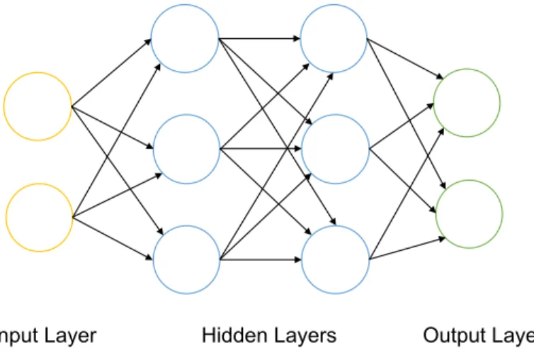
A Multi-Layer Perceptron (MLP) is a feedforward artificial neural network that consists of multiple layers of nodes in a directed graph where each layer is fully connected to the next one. Figure 5 is a MLP illustration with two hidden fully connected layers.
A MLP classifier trains iteratively because at each time step the partial derivatives of the loss function with respect to the model parameters are computed to update parameters.
In this study, five MLP variants are derived. The different implementations explore various model architectures (i.e. number of layers and number of neurons) and different activation functions. Identity, ReLU (Rectified Linear Unit) and Logistic are three types of activation function that are investigated.30 The first three models use a single hidden layer, whereas the last two respectively use two and three hidden layers. The activation function chosen for the deep neural networks (i.e. more than one hidden layer) is selected based on the performance of the single layered MLPs. All MLPs are trained using an SGD algorithm. Because parameters are updated after each propagation, mini batches of size 32 are used in order to speed up the neural network training. The learning rate is tuned for the models such that it balances overshooting and
Hidden Layers
Input Layer Output Layer
Figure 5. Multi-Layer Perceptron (MLP) with Two Hidden Layers
slow convergence. The training ends when the first stopping criteria is met, which is defined by a maximum of 5000 iterations or a tolerance of less than 0.0001.
Table 3 summarizes the five MLP model and architecture variants.
Table 3. Multi-Layer Perceptron Model and Architecture Variants
MLP Number of Layers Number of Neurons Activation Function Learning Rate
MLP-1-Id 1 100 Identity 0.001
MLP-1-R 1 100 ReLU 0.01
MLP-1-L 1 100 Logistic 0.01
MLP-2-Id 2 100, 100 ReLU 0.01
MLP-3-R 3 100, 100, 100 ReLU 0.01
2. Convolutional Neural Network (CNN)
A Convolutional Neural Network (CNN) is similar to a MLP but makes the assumption that the inputs can be represented as images, usually represented by matrices. Three types of hidden layers are used to build a CNN: Convolutional Layer (CL), Pooling Layer (PL), and Fully-Connected Layer (FCL). Figure 6 illustrates the three CNN layer types, given an input image.
Figure 6. Convolutional Neural Network (CNN)
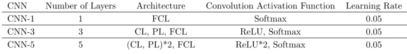
Three CNN architectures are explored with respectively one, three, and five hidden layers. Table 4 summarizes the three CNN models and architecture variants. In all models, mini batches of size 64 are used
to perform gradient descent (SGD algorithm) during training. The learning rate is tuned for the models such that it balances overshooting and slow convergence. A number between 10 and 15 epochs is used for training in order to let the algorithm reach large accuracy values (i.e. greater than 90%). For both CNN with three and five hidden layers, a max Pooling Layer (PL) connects the Convolutional Layer (CL) to the next hidden layer to reduce the dimensionality of the feature map created by the CL. The CL applies an activation function, typically RELU i.e. Rectified Linear Units, to introduce non-linearities into the model and prevent linear model response to the variables. The last layer named the Fully-Connected Layer (FCL), performs the classification on the features extracted by the convolution/pooling layers and returns the raw values for the predictions using four neurons, a neuron per target class of the model, i.e. per feasible landing runway. The softmax activation function generates values between 0 and 1 for each neuron of the FCL which can be interpreted as relative measurements of how likely the input image falls into each target class.
Table 4. Convolutional Neural Network Model and Architecture Variants
CNN Number of Layers Architecture Convolution Activation Function Learning Rate
CNN-1 1 FCL Softmax 0.05
CNN-3 3 CL, PL, FCL ReLU, Softmax 0.05
CNN-5 5 (CL, PL)*2, FCL ReLU*2, Softmax 0.05
C. Implementation
The different algorithms and classifiers are implemented using Python as the programming language and using the Scikit-learn and TensorFlow libraries.23, 31 The training and testing were executed on a Macintosh
platform with 2.5GHz Intel Core i7 and 16GB RAM.
IV.
Results
The previously described classifiers are run to solve the runway recognition problem for the DFW appli-cation. Three analyses are conducted in order to understand and exploit the capabilities of the classifiers, and the results are presented in this section. To compare the algorithm performances, several metrics are computed such as the prediction accuracy, the training and testing times. The analysis starts with predic-tion results of models that were trained using one track data point per trajectory, where a track data point encompasses the values of the ten selected features at a particular time step. Then results obtained with models trained using minutes of track data point per trajectory are detailed.
A. Prediction Analysis
The prediction analysis focuses on investigating the feasibility of predicting the landing runway with the ten selected features and with one track data point per trajectory, and characterizing how close to the runway that point must be to obtain accurate predictions. The results of the analysis compare the classifier performances in terms of accuracy, training and testing times on predicting the correct landing runway. It is assumed that an observer close to the runway is able to predict the landing runway with higher accuracy than an observer far from the runway. To run the analysis, two datasets are created from the main dataset. For both datasets, the original trajectory input set is reduced to track data point input sets respectively representing the trajectory information of all flights at three and ten minutes from landing. The resulting datasets can be referred as Dataset 3min and Dataset 10min. For learning purposes, the considered datasets are randomly split into training and testing sets of size 2/3 and 1/3 of the original datasets such that each subset gets at least 25% of the total number of arrival flights for each runway.
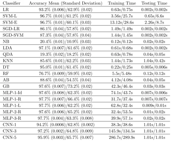
Table 5 summarizes the classification results for each dataset, and all supervised learning algorithm performance results are included. For each machine learning non-ensemble method, a 10-fold cross validation procedure was implemented, and associated training and testing times are reported in Table 5. For all other methods, the training was performed on ten different training sets, and performance average distributions were computed.
Table 5. Classification Accuracy and Time Summary Dataset 3min/Dataset 10min
Classifier Accuracy Mean (Standard Deviation) Training Time Testing Time LR 93.2% (0.006)/62.9% (0.02) 0.63s/0.75s 0.002s/0.002s SVM-L 96.7% (0.01)/61.2% (0.02) 3.56s/25.7s 0.65s/6.6s SVM-E 96.7% (0.01)/60.1% (0.03) 13.12s/28.6s 2.26s/8.7s SGD-LR 86.1% (0.04)/57.8% (0.02) 1.49s/1.49s 0.002s/0.002s SGD-SVM 87.3% (0.04)/57.8% (0.04) 1.44s/1.45s 0.002s/0.002s NB 20.4% (0.01)/10.9% (0.03) 0.12s/0.12s 0.02s/0.02s LDA 97.1% (0.007)/61.6% (0.02) 0.61s/0.68s 0.002s/0.002s QDA 19.3% (0.02)/18.2% (0.02) 0.63s/0.78s 0.04s/0.05s KNN 85.6% (0.01)/62.2% (0.03) 1.44s/1.73s 1.04s/0.42s DT 95.0% (0.01)/61.4% (0.02) 0.22s/0.25s 0.005s/0.006s RF 76.7% (0.009)/59.9% (0.02) 5.5s/5.48s 0.12s/0.12s AB 88.6% (0.04)/54.5% (0.04) 4.12s/4.08s 0.04s/0.05s GB 97.6% (0.007)/73.2% (0.02) 42.3s/46.4s 0.03s/0.03s MLP-1-Id 97.6% (0.008)/62.3% (0.02) 74.1s/43.7s 0.007s/0.006s MLP-1-R 97.7% (0.007)/66.4% (0.02) 31.7s/37.4s 0.007s/0.007s MLP-1-L 97.7% (0.006)/62.2% (0.02) 62.8s/32.4s 0.009s/0.01s MLP-2-R 97.6% (0.006)/65.2% (0.02) 32.4s/53.5s 0.01s/0.02s MLP-3-R 97.7% (0.004)/63.3% (0.008) 39.9s/57.1s 0.02s/0.02s CNN-1 94.2% (0.0006)/62.8% (0.002) 38.3s/38.6s 1.01s/1.01s CNN-3 97.2% (0.002)/64.8% (0.009) 145.9s/134.5s 1.01s/1.01s CNN-5 95.9% (0.003)/65.7% (0.007) 286.7s/289.9s 1.01s/1.01s
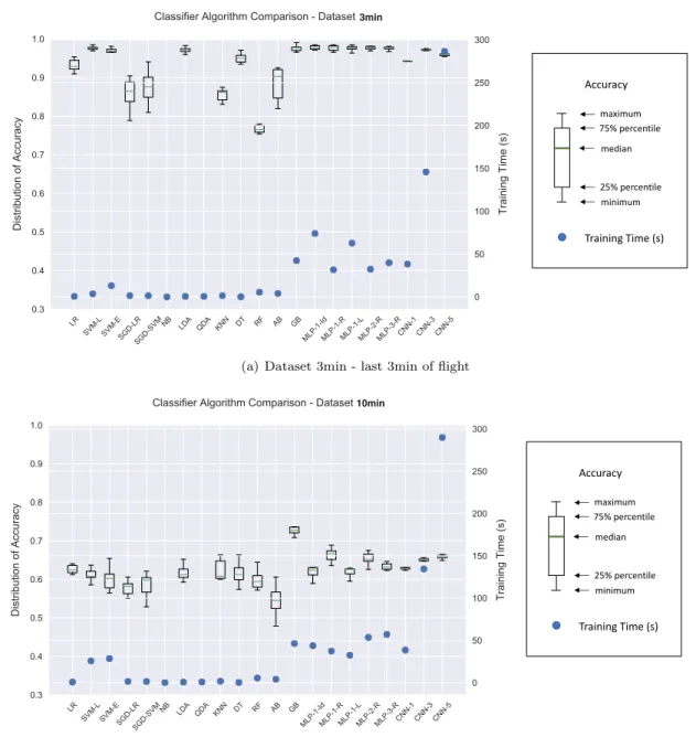
Figure 7 illustrates the performance result distributions in terms of accuracy and training time, and compares them for the two datasets. The acronyms of each classifier are defined in the previous section. For each classifier, a box-and-whisker plot visualization is chosen to represent the accuracy distribution, which values can be observed on the left y-axis. Box-and-whisker diagrams are standardized forms to illustrate data distribution. The bottom and top of the box, respectively, represent the 25th and 75th percentiles, and the line inside the box denotes the median. The bottom and top whiskers indicate the minimum and maximum values of the data considered. To show the variations of successful classifiers, the lower accuracy value limit was intentionally set to 0.3. The right y-axis represents the time scale.
Overall and for all classifiers, Table 5 and Figure 7 show higher levels of accuracy for Dataset 3min than for Dataset 10min. The results obtained are thus in conformance with initial expectations. For both datasets, QDA and NB classifiers performed the worst, with accuracy mean values less than 20%, and are thus not represented in Figure 7. For the classifiers of the ensemble methods family, RF provides the worst accuracy results, respectively giving 76.7% and 59.9% accuracy for Dataset 3min and Dataset 10min, whereas GB provides the best results, respectively giving 97.6% and 73.2% accuracy for Dataset 3min and Dataset 10min. Additionally, regardless of the dataset, all linear classifiers (i.e. LR, SVM-L, LDA) and neural networks provide accuracy mean results in the range of 93.2% to 97.7% for Dataset 3min, and 62.2% to 66.4% for Dataset 10min. These results demonstrate that the algorithm decision boundaries have linear properties which explains the lower accuracy results computed with QDA. The results also show that the selected features are not all mutually independent and present some interdependences, hence the predictions obtained with NB do not present high levels of accuracy. Moreover, the accuracy results demonstrate that all investigated neural network variants behave very similarly in terms of mean values, respectively above 94% and 62% for Dataset 3min and Dataset 10min, and standard deviation values, respectively less than 0.01 and 0.02 for Dataset 3min and Dataset 10min. Over all classifiers, GB provides the best results for both datasets in terms of accuracy.
3min Accuracy maximum minimum 75% percentile median 25% percentile Training Time (s)
(a) Dataset 3min - last 3min of flight
Accuracy maximum minimum 75% percentile median 25% percentile Training Time (s) 10min
(b) Dataset 10min - last 10min of flight
Figure 7. Machine Learning Classifier Algorithm Comparison
290s. Linear classifiers, DT and KNN take an order of magnitude less time to train than most classifiers of the ensemble methods (RF, AB, GB) and neural networks (all MLPs and CNN-1) with the exception of the convolutional neural networks with more than one layer, CNN-3 and CNN-5, that take two orders of magnitude more time to train. It is interesting to notice than SVMs are the only tested classifiers that are affected by using different datasets. In particular, the SVM results show that SVM-L is faster than SVM-E and that when training the classifiers with Dataset 10min, the required training times respectively increase by 5 for SVM-L and by 2 for SVM-E. On one hand, the computation of the SVM-L linear kernel matrix takes less time than the computation of the non-linear kernel for SVM-E. And on the other hand, the track data points describing the trajectories ten minutes from landing overlap more than three minutes from landing which increase the difficulty of the SVM algorithms to find the hyper-planes that segregate the input data to classes. Moreover, when looking closely at the neural network training time results, it can be observed that MLP-1-Id and MLP-1-L take less time to be trained with Dataset 10min than with Dataset 3min. However, these results are within the overall range of neural network training times and not
outliers. When comparing with the other neural networks, the differences in training times can be attributed to the selection of activation functions, and different computation behaviors were accordingly expected. In particular, since no obvious difference can be observed in terms of accuracy, the neural network results show that when the ReLU activation function is applied, better performance in accuracy variance and training time are computed than with other activation functions.
Moreover, it can be noticed that although high levels of accuracy are demonstrated for both datasets, SGD-LR and SGD-SVM classifiers show the highest levels of accuracy variability. Figure 7 illustrates that for all classifiers, higher accuracy variability is computed with Dataset 10min than with Dataset 3min. This reinforces the expectation that more accurate and certain landing runway predictions can be computed when closer to the runways.
When closely analyzed, the results illustrate a broad spectrum of behaviors amongst the classifiers that reflects the intrinsic characteristics of the considered datasets and the chosen algorithm parameter values. For this application and the selected features regardless of the dataset, neural network models perform better than non-neural network classifiers in terms of accuracy mean and results robustness (i.e. less variability over the different datasets). However, as observed in the results, this comes at the price of higher training times. Finally, the results obtained with the CNN classifiers validate the assumption that the trajectory track points used as inputs in this application can be represented as images and are well suited for convolution operations. Overall, GB gives the best compromise of all classifiers giving high levels of accuracy with low levels of variability for both datasets at reasonable training times of about 42 to 46 seconds.
B. Sensitivity Analysis
In order to challenge the results of the prediction analysis and exploit the different classifiers, a sensitivity analysis is conducted to understand if the levels of accuracy previously computed for Dataset 10min can be improved by training the classifiers using more information. In particular, the number of data points provided as inputs for the training is incrementally increased. The goal of this analysis is to investigate the sensitivity of each classifier with respect to the amount of data used in training. The analysis starts by training the classifiers using the furthest point out from the runway, i.e. ten minutes away, and incrementally continues by adding more track points in the direction of the runway. Starting with Dataset 10min and augmenting the dataset with longer time series, Figure 8 illustrates the results of the analysis, and results are reported every twelve sets of data points spaced every five seconds, i.e. every minute.
Figure 8(a) and Figure 8(b) respectively represent the average mean accuracy and average training time after cross validation in function of the number of data points provided as input starting ten minutes out from the runway. To lighten the plot, the number of minutes is limited to eight (i.e. 0 to 7 minutes), which is enough to obtain accuracy values higher then 90% for most classifiers. In this analysis, CNNs results with more than three layers are not reported because the required training time to reach 90% is of a larger order of magnitude than with all other classifiers.
Figure 8(a) illustrates as in Subsection A that QDA and NB are the worst classifiers for all time steps, and in particular they do not reach satisfactory levels of accuracy (i.e. 50%) even when trained using time series containing track data points covering ten to three minutes from landing. However, and similarly to the rest of the implemented classifiers, when the number of track data points used for training is increased, the computed accuracy levels improve. In particular when time series containing track data points down to three minutes from landing are used for training, all remaining classifiers reach accuracy levels greater than 75%. The relationship between mean accuracy and number of minutes provided as input presents linear improvement characteristics for all classifiers of about 10% between 0 to 4 minutes and of about 25% between 4 and 7 minutes. GB demonstrates the best accuracy results for all time steps.
Figure 8(b) displays the impact of adding more time steps into training in terms of computation time. The results for the neural network models show that they are not sensitive to the number of minutes and show constant training times. On the contrary, the linear and ensemble family-based classifiers are sensitive to the number of track data points used during training, in particular they all see their training times increase from 15 times for GB to 150 times for LR. It takes more than 1000 seconds to train the GB classifier with time series input covering trajectories down to three minutes before landing. Moreover, although a slight training time increase is observed when comparing the two extreme input time series, 0 and 0-to-7 minutes, SVM-based classifiers demonstrate that the more data used as input the more efficient and fast they are at training.
0 1 2 3 4 5 6 7
Minutes of Input Data
0.2 0.3 0.4 0.5 0.6 0.7 0.8 0.9 1.0 Accuracy Mean LR SVM-L SVM-E SGD-LR SGD-SVM NB LDA QDA KNN DT RF AB GB MLP-1-Id MLP-1-R MLP-1-L MLP-2-R MLP-3-R CNN-1
Sensitivity Analysis - Accuracy Mean
(a) Sensitivity Analysis - Accuracy Mean
0 1 2 3 4 5 6 7
Minutes of Input Data
0 200 400 600 800 1000
Cross Validation Time (s)
LR SVM-L SVM-E SGD-LR SGD-SVM NB LDA QDA KNN DT RF AB GB MLP-1-Id MLP-1-R MLP-1-L MLP-2-R MLP-3-R CNN-1
Sensitivity Analysis - Timing
(b) Sensitivity Analysis - Time (s)
Figure 8. Sensitivity Analysis - the first data point is 10 minutes away from the runway threshold, the following data points are 10 - x minutes away from the runway threshold where x is minutes of input data
feature time series, whereas neural network models are able to intrinsically adjust their neuron weights to integrate the temporal aspect of the input data. As observed in the results, this does present advantages because no net training time change is observed for the neural network models.
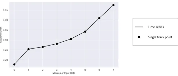
Finally, the results of the sensitivity analysis demonstrate that the classifiers are sensitive to the distance of the track points given as input from the landing runways and that higher accuracy levels can be computed when longer time series are used as input but at higher training time costs. However when comparing the sensitivity results computed at ten and three minutes from landing with the ones obtained in the prediction analysis in Subsection A, the past information provided in lengthier time series in this analysis does not seem to influence the accuracy results. Instead a single track data point per trajectory seems sufficient to predict the landing runway with decent levels of accuracy. In particular, Figure 9 illustrates the mean accuracy
results for GB when the input data is constituted of time series of different lengths versus single track data points at different times. The black dots represent the accuracy results computed when the input data is constituted of single track point data for each trajectory.
Time series Single track point
Figure 9. Gradient Boosting (GB) - Time Series Input Data vs Single Track Point Input Data
Figure 9 demonstrates that the computed accuracy results are similar regardless if past information is provided as input. Therefore, it can be concluded that when time series are used to train the classifiers, the closest track point to the runway is the one mainly indicative for the outcome classification.
C. Feature Importance Analysis
An analysis of feature importance enables one to find and select the most impactful features on the classi-fication results. The Gradient Boosting GB classifier is selected to run the study since it provided the best prediction results and thanks to its graph representation that enables simple feature extraction. Generally, importance provides a score that indicates how valuable each feature was in the construction of the boosted decision trees within the model. The higher, the more important the feature to make key decisions with decision trees.32 In the GB implementation selected for this study, the Gini index is used as the performance measure to compute the quality of splits. Importance is calculated for a single decision tree by computing the amount of each feature split point improves the performance measure and is weighted by the number of observations the node is responsible for. Because GB uses multiple trees, the feature importances are then averaged across all of the decision trees within the model.
Since the problem deals with ten features, the goal of this analysis isn’t to necessarily reduce the number of considered features but to understand if there exists any feature dominance. Dataset 10min contains the last ten minutes of flight times, which represents 120 time steps spaced every five seconds. In order to also explore the temporal impact on the classification, three cases are investigated for the analysis that respectively use three different temporal input data.
In the first case, the input data are constituted of Dataset 3min containing track data points located three minutes from landing, i.e. at time step 35. In the second case, the entire dataset, i.e. for each aircraft, all trajectory time steps, 1-119, are provided as input. And in the third case, Dataset 10min including track data points situated ten minutes from landing, i.e. at time step 119, is given as input.
Figure 10 illustrates the results of the analysis for the three cases. The purple bars represent the feature importances of the classifier, and their values are displayed on the y-axis. In all cases, the ten most dominant features are reported.
On one hand, Figure 10(a) shows that for Case 1 two features-latitude and ground speed, in this order-dominate during training. When training the classifier using data points close to the runway, altitude and course angle conditions do not influence as much the classification of the landing runways. It is to be noticed that in the DFW application, the feeder gate YEAGER does influence the classification, and this is
Latitude_35 GroundSpeed_35
FeederGateYEAGR_35
RateOfClimb_35Altitude_35Longitude_35Course_35AirlineSRY_35AirlineUAL_35AirlineMRA_35
0.0 0.1 0.2 0.3 0.4
(a) Case 1 - Time Step 35
Longitude_1Longitude_3Longitude_0Longitude_8Longitude_6Longitude_10Longitude_9Latitude_0Longitude_4Longitude_5
0.00 0.01 0.02 0.03 0.04 0.05 0.06 0.07 0.08
(b) Case 2 - Time Steps 1-119, Complete Time Series
Longitude_119Course_119Latitude_119Altitude_119
GroundSpeed_119RateOfClimb_119AirlineENY_119AirlineASH_119 WeightCategoryH_119 AirlineNKS_119 0.00 0.05 0.10 0.15 0.20 0.25
(c) Case 3 - Time Step 119 Figure 10. Feature Importance
explained by the considered set of trajectories that enters the TRACON using that gate. On the other hand, Figure 10(c) demonstrates that for Case 3, the longitude is primarily dominating the other features, and it is followed by the course angle, the latitude, the altitude and the ground speed. When training the classifier using data points points far from the runway, the longitude is key in distinguishing and classifying the landing runway. For Case 2 illustrated in Figure 10(b), the longitude dominates all other features, regardless of the time step. Case 2 also shows that the temporal nature of the input features does not impact the results because the longitude values measured close to the runway are more impactful than values measured further out. The layout of DFW airport runways clearly shows that the runways are located at the same altitude and latitude. However they have a different longitude which explains why, in all three cases, the longitude is a dominant feature.
V.
Summary, Conclusion and Applications
Given the recent increase of autonomous systems development with supervised learning algorithms, this paper explored a collection of supervised learning algorithms to solve a trajectory classification problem in the field of Air Traffic Management. In particular, it focused on a runway recognition problem formulated as the prediction of landing runways given historical aircraft trajectories. Several machine learning classifiers were applied to different datasets. Performance metrics such as accuracy, training and testing times were computed.
The results showed that, as to be expected, for all investigated classifiers, the accuracy results were better for Dataset 3min than for Dataset 10min, respectively, representing trajectory points three and ten minutes from landing. This confirmed the expectation that an observer closer to the runway is more likely to identify correctly the landing runway than an observer positioned further out. Moreover, the prediction
analysis showed that for Dataset 3min, high accuracy levels above 90% were achieved using one track data point per trajectory, whereas decreased accuracy levels closer to 60% were obtained for Dataset 10min. A diverse spectrum of training times was computed amongst the classifiers – the linear, decision tree and k-nearest neighbors classifiers took an order of magnitude less time to train than most classifiers of the ensemble methods and neural networks. Moreover, although most classifiers needed similar training times for both datasets, the support vector machine classifiers were affected by the change of training dataset. The gradient boosting classifier presented the highest performance, balancing accuracy and training time for both datasets.
Additionally, a sensitivity analysis was conducted to understand the impact of adding more information during training, i.e. more time steps, to predict the landing runway with high accuracy. The levels of accuracy obtained by the classifiers kept improving as the track data points got closer to the runways. The results in terms of training times were slightly different and the classifiers behaved differently with the increased number of track data points. The neural networks showed that they were not sensitive to the number of minutes, whereas the linear and ensemble family-based classifiers saw their training times increased from 15 times to 150 times. Moreover, support vector machine classifiers demonstrated that the more data used as input the more efficient and fast they were at training. The sensitivity analysis also demonstrated that the added information contained in the input time series did not increase significantly the computed levels of accuracy. Instead, similar accuracy levels were computed for all classifiers when individual track data points were used as input.
Finally, a feature importance analysis was performed using the gradient boosting model to visualize feature dominance. Of the three cases studied, the longitude feature dominated the other considered features. However, the machine learning classifier did not utilize the temporal information from the time series and showed that when the entire dataset was used for training, the information from the time steps close to the runway dominated over the others.
This paper shows encouraging results on applying supervised learning techniques to a specific trajectory problem, and this exploratory piece of work could provide information and guidance in other future Air Traffic Management classification endeavours. Practical applications of this study extend, for example, to the prediction of package delivery locations given that the information is not available and the prediction of air traffic controller intentions in conflict resolution maneuvers given historical aircraft trajectories.
In the context of research in autonomy, an autonomous air traffic control system such as the proposed Terminal Area Automated Concept (TAAC) could benefit from such a predictive module by providing TAAC the most likely preferred runway, if the information is not available, when the aircraft first enters the TRACON airspace. TAAC would then use the predicted assignment as the preferred runway or use it as the runway when searching for a runway assignment that produces the least delay. Moreover, in the context of current air traffic control, the methodology developed in this study could also be used as part of a pilot and/or air traffic controller technology that detects trajectory deviations. In particular, as an aircraft gets closer to landing, given its positions and the demonstrated increased accuracy predictions close to the runways, the algorithm could provide a probability of landing on the assigned runway and trigger an alarm in case the probability falls below a specified threshold, thus identifying an aircraft-runway misalignment.
VI.
Acknowledgments
The authors would like to thank Dr. Todd Lauderdale, Dr. Heinz Erzberger, Dr. Antony Evans, Dr. Todd Farley and Dr. Banavar Sridhar for their support and feedback during the research and writing of this paper.
References
1Nikoleris, T., Erzberger, H., Paielli, R. A., and Chu, Y.-C., “Autonomous system for air traffic control in terminal
airspace,”proceedings of 14th AIAA Aviation Technology, Integration, and Operations Conference (ATIO 2014), Atlanta, GA,
USA, 2014.
2Mahboubi, Z. and Kochenderfer, M. J., “Autonomous air traffic control for non-towered airports,”Proc. USA/Europe
Air Traffic Management Research Development Seminar, 2015, pp. 1–6.
3Xu, N., Donohue, G., Laskey, K. B., and Chen, C.-H., “Estimation of delay propagation in the national aviation system
using Bayesian networks,”6th USA/Europe Air Traffic Management Research and Development Seminar, 2005.
4Rebollo, J. J. and Balakrishnan, H., “Characterization and prediction of air traffic delays,”Transportation research part
5Choi, S., Kim, Y. J., Briceno, S., and Mavris, D., “Prediction of weather-induced airline delays based on machine learning
algorithms,”Digital Avionics Systems Conference (DASC), 2016 IEEE/AIAA 35th, IEEE, 2016, pp. 1–6.
6Gariel, M., Srivastava, A. N., and Feron, E., “Trajectory clustering and an application to airspace monitoring,”IEEE
Transactions on Intelligent Transportation Systems, Vol. 12, No. 4, 2011, pp. 1511–1524.
7Gopalakrishnan, K., Balakrishnan, H., and Jordan, R., “Clusters and communities in air traffic delay networks,”American
Control Conference (ACC), 2016, IEEE, 2016, pp. 3782–3788.
8Conde Rocha Murca, M., DeLaura, R., Hansman, R. J., Jordan, R., Reynolds, T., and Balakrishnan, H., “Trajectory
Clustering and Classification for Characterization of Air Traffic Flows,” 16th AIAA Aviation Technology, Integration, and
Operations Conference, 2016, p. 3760.
9Arneson, H., “Initial analysis of and predictive model development for weather reroute advisory use,”15th AIAA Aviation
Technology, Integration, and Operations Conference, 2015, p. 3395.
10Evans, A. D. and Lee, P. U., “Predicting the Operational Acceptability of Route Advisories,” 17th AIAA Aviation
Technology, Integration, and Operations Conference, 2017, p. 3078.
11Bloem, M. and Bambos, N., “Ground Delay Program analytics with behavioral cloning and inverse reinforcement
learn-ing,”Journal of Aerospace Information Systems, 2015.
12Najafabadi, M. M., Villanustre, F., Khoshgoftaar, T. M., Seliya, N., Wald, R., and Muharemagic, E., “Deep learning
applications and challenges in big data analytics,”Journal of Big Data, Vol. 2, No. 1, 2015, pp. 1.
13Hinton, G., Deng, L., Yu, D., Dahl, G. E., Mohamed, A.-r., Jaitly, N., Senior, A., Vanhoucke, V., Nguyen, P., Sainath,
T. N., et al., “Deep neural networks for acoustic modeling in speech recognition: The shared views of four research groups,” IEEE Signal Processing Magazine, Vol. 29, No. 6, 2012, pp. 82–97.
14Krizhevsky, A., Sutskever, I., and Hinton, G. E., “Imagenet classification with deep convolutional neural networks,”
Advances in neural information processing systems, 2012, pp. 1097–1105.
15Deng, L. and Yu, D., “Deep Learning: Methods and Applications,”Found. Trends Signal Process., Vol. 7, No. 3–4,
June 2014, pp. 197–387.
16Fakoor, R., Ladhak, F., Nazi, A., and Huber, M., “Using deep learning to enhance cancer diagnosis and classification,”
Proceedings of the International Conference on Machine Learning, 2013.
17Ding, X., Zhang, Y., Liu, T., and Duan, J., “Deep Learning for Event-Driven Stock Prediction.” IJCAI, 2015, pp.
2327–2333.
18Lv, Y., Duan, Y., Kang, W., Li, Z., and Wang, F.-Y., “Traffic flow prediction with big data: a deep learning approach,”
IEEE Transactions on Intelligent Transportation Systems, Vol. 16, No. 2, 2015, pp. 865–873.
19Kim, Y. J., Choi, S., Briceno, S., and Mavris, D., “A deep learning approach to flight delay prediction,”Digital Avionics
Systems Conference (DASC), 2016 IEEE/AIAA 35th, IEEE, 2016, pp. 1–6.
20Erzberger, H., Nikoleris, T., Paielli, R. A., and Chu, Y.-C., “Algorithms for control of arrival and departure traffic in
terminal airspace,”Proceedings of the Institution of Mechanical Engineers, Part G: Journal of Aerospace Engineering, Vol. 230,
No. 9, 2016, pp. 1762–1779.
21Nikoleris, T., Erzberger, H., Paielli, R. A., and Chu, Y.-C., “Performance of an Automated System for Control of Traffic
in Terminal Airspace,” 2016.
22National Transportation Safety Board, “Landing Approach to Taxiway at San Francisco International Airport (SFO),”
2017,https://www.ntsb.gov/investigations/Pages/DCA17IA148.aspx(accessed September 22, 2017).
23Pedregosa, F., Varoquaux, G., Gramfort, A., Michel, V., Thirion, B., Grisel, O., Blondel, M., Prettenhofer, P., Weiss, R.,
Dubourg, V., Vanderplas, J., Passos, A., Cournapeau, D., Brucher, M., Perrot, M., and Duchesnay, E., “Scikit-learn: Machine
Learning in Python,”Journal of Machine Learning Research, Vol. 12, 2011, pp. 2825–2830.
24Blum, A. L. and Langley, P., “Selection of relevant features and examples in machine learning,”Artificial intelligence,
Vol. 97, No. 1, 1997, pp. 245–271.
25Guyon, I. and Elisseeff, A., “An introduction to variable and feature selection,”Journal of machine learning research,
Vol. 3, No. Mar, 2003, pp. 1157–1182.
26Federal Aviation Administration, “DFW Airport Capacity Profile,” 2014, https://www.faa.gov/airports/planning_
capacity/profiles/media/DFW-Airport-Capacity-Profile-2014.pdf(accessed May 26, 2017).
27Bureau of Transportation Statistics, “On-Time : On-Time Performance,” 2016,https://www.transtats.bts.gov/DL_
SelectFields.asp?Table_ID=236&DB_Short_Name=On-Time(accessed May 26, 2017).
28Eshow, M. M., Lui, M., and Ranjan, S., “Architecture and capabilities of a data warehouse for ATM research,”Digital
Avionics Systems Conference (DASC), 2014 IEEE/AIAA 33rd, IEEE, 2014, pp. 1E3–1.
29Segaran, T.,Programming collective intelligence: building smart web 2.0 applications, ” O’Reilly Media, Inc.”, 2007.
30Goodfellow, I., Bengio, Y., and Courville, A.,Deep learning, MIT Press, 2016.
31Abadi, M., Agarwal, A., Barham, P., Brevdo, E., Chen, Z., Citro, C., Corrado, G. S., Davis, A., Dean, J., Devin, M.,
Ghemawat, S., Goodfellow, I., Harp, A., Irving, G., Isard, M., Jia, Y., Jozefowicz, R., Kaiser, L., Kudlur, M., Levenberg, J.,
Man´e, D., Monga, R., Moore, S., Murray, D., Olah, C., Schuster, M., Shlens, J., Steiner, B., Sutskever, I., Talwar, K., Tucker,
P., Vanhoucke, V., Vasudevan, V., Vi´egas, F., Vinyals, O., Warden, P., Wattenberg, M., Wicke, M., Yu, Y., and Zheng, X.,
“TensorFlow: Large-Scale Machine Learning on Heterogeneous Systems,” 2015, Software available from tensorflow.org.
32Friedman, J., Hastie, T., and Tibshirani, R.,The elements of statistical learning, Vol. 1, Springer series in statistics New