Converting to Optimization in Machine Learning: Perturb-and-MAP, Differential Privacy, and Program Synthesis

(1)

Converting to Optimization in

Machine Learning:

Perturb-and-MAP, Differential

Privacy, and Program Synthesis

Matej Balog

Department of Engineering

University of Cambridge

This thesis is submitted for the degree of

Doctor of Philosophy

(2)

(3)

Declaration

This thesis is the result of my own work and includes nothing which is the outcome of work done in collaboration except as declared in the Preface and specified in the text. It is not substantially the same as any that I have submitted, or, is being concurrently submitted for a degree or diploma or other qualification at the University of Cambridge or any other University or similar institution except as declared in the Preface and specified in the text. I further state that no substantial part of my thesis has already been submitted, or, is being concurrently submitted for any such degree, diploma or other qualification at the University of Cambridge or any other University or similar institution except as declared in the Preface and specified in the text. It does not exceed the prescribed word limit for the relevant Degree Committee.

Matej Balog February 2020

(4)

(5)

Converting to Optimization in Machine Learning:

Perturb-and-MAP, Differential Privacy, and

Program Synthesis

Matej Balog

On a mathematical level, most computational problems encountered in machine learning

are instances of one of four abstract, fundamental problems: sampling, integration,

optimization, andsearch. Thanks to the rich history of the respective mathematical

fields, disparate methods with different properties have been developed for these four problem classes. As a result it can be beneficial to convert a problem from one abstract class into a problem of a different class, because the latter might come with insights, techniques, and algorithms well suited to the particular problem at hand. In particular, this thesis contributes four new methods and generalizations of existing methods for converting specific non-optimization machine learning tasks into optimization problems with more appealing properties.

The first example is partition function estimation (anintegrationproblem), where an

existing algorithm – theGumbel trick– for converting to the MAPoptimization problem

is generalized into a more general family of algorithms, such that other instances of this family have better statistical properties. Second, this family of algorithms is further

generalized to another integration problem, the problem of estimating Rényi entropies.

The third example shows how an intractablesampling problem arising when wishing to

publicly release a database containing sensitive data in a safe (“differentially private”)

manner can be converted into anoptimization problem using the theory of Reproducing

Kernel Hilbert Spaces. Finally, the fourth case study casts the challenging discrete

search problem of program synthesis from input-output examples as a supervised

learning task that can be efficiently tackled using gradient-based optimization.

In all four instances, the conversions result in novel algorithms with desirable properties. In the first instance, new generalizations of the Gumbel trick can be used to construct statistical estimators of the partition function that achieve the same estimation error while using up to 40% fewer samples. The second instance shows that unbiased estimators of the Rényi entropy can be constructed in the Perturb-and-MAP framework. The main contribution of the third instance is theoretical: the conversion shows that it is possible to construct an algorithm for releasing synthetic databases that approximate databases containing sensitive data in a mathematically precise sense,

(6)

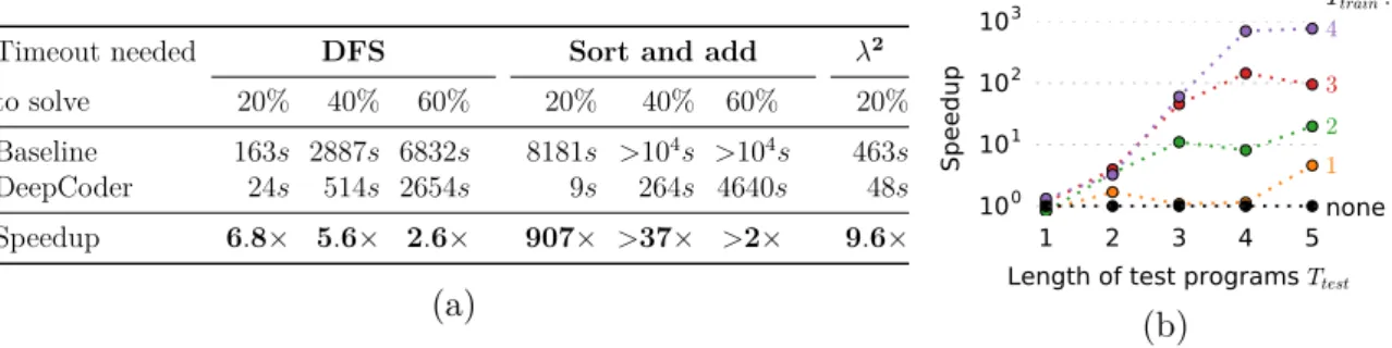
and to prove results about their approximation errors. Finally, the fourth conversion yields an algorithm for synthesising program source code from input-output examples that is able to solve test problems 1-3 orders of magnitude faster than a wide range of baselines.

(7)

Acknowledgements

My biggest thanks go to my family and friends who have supported me on this journey. Its academic component also would not have been possible without the dedicated teachers at Gymnázium Grösslingová in Bratislava, and the brilliant tutors and lecturers at Merton College and the Mathematics, Statistics, and Computer Science departments in Oxford.

I would like to thank Zoubin Ghahramani, Bernhard Schölkopf, and Carl E. Ras-mussen for giving me the opportunity to embark on this PhD programme, and for supporting me along the way, providing both guidance and freedom as needed. I’m particularly grateful to Bernhard Schölkopf for the unique chance to visit the world-class Max-Planck-Institute in Intelligent Systems in Tübingen, and for making sure I had a valuable research experience there.

A most enriching part of the PhD programme have been collaborations with many wonderful colleagues – Nilesh Tripuraneni, Rishabh Singh, and Danny Tarlow – among many others. Thank you all!

Finally, I would like to highlight friends who have supported me all the way along this journey both personally and academically: Tuan Anh Le, George Hron, thank you.

(8)

(9)

List of figures

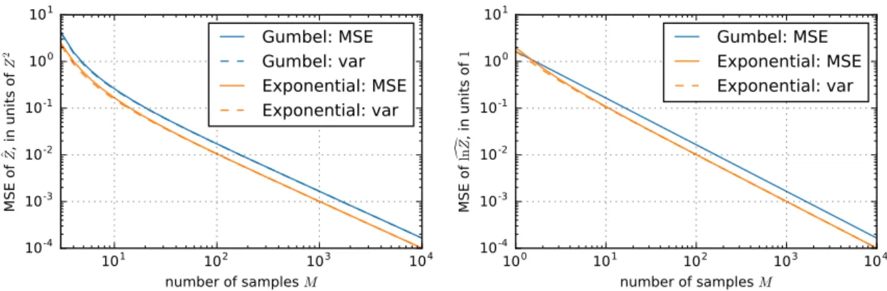
2.1 Analytically computed MSE and variance of Gumbel and Exponential trick estimators of Z (left) and lnZ (right). The MSEs are dominated by the variance, so the dashed and solid lines mostly overlap. See Section 2.2.3 for details. . . 37

2.2 MSE of estimators ofZ (left) and lnZ (right) stemming from Fréchet (−1₂ < α <0), Gumbel (α = 0) and Weibull tricks (α >0). See Section 2.2.3 for details. . . 37

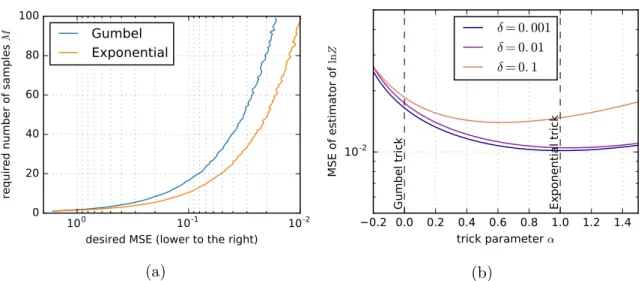
2.3 (a) Sample size M required to reach a given MSE using Gumbel and Ex-ponential trick estimators of lnZ, using samples from A∗ sampling (see Section 2.5.1) on a Robust Bayesian Regression task. The Exponential trick is more efficient, requiring up to 40% fewer samples to reach a given MSE. (b) MSE of lnZ estimators for different values ofα, usingM = 100 samples from the approximate MAP algorithm discussed in Section 2.5.2, with different error boundsδ. For small δ, the Exponential trick is close to optimal, match-ing the analysis of Section 2.2.3. For larger δ, the Weibull trick interpolation between the Gumbel and Exponential tricks can provide an estimator with lower MSE. . . 46

(14)

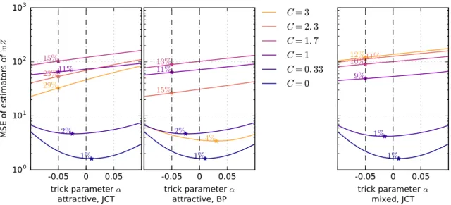
2.4 MSEs of U(α) as estimators of lnZ on 10×10 attractive (left, middle) and mixed (right) spin glass model with different coupling strengthsC (see Section 2.5.3). We also show the percentage of samples saved by using the bestα in place of the Gumbel trick estimatorU(0), assuming the asymptotic regime. For this we only consideredα >−1/(2√n) =−0.05, where variance is provably finite, see Section 2.3.1. The MAP problems were solved using the exact junction tree algorithm (JCT, left and right), or approximate belief propagation (BP, middle). In all cases, when coupling is very low,α close to 0 is optimal. This also holds for BP when coupling is high. In other regimes, upper bounds derived from the Fréchet trick, i.e. α < 0, provide more accurate estimators. . . 47

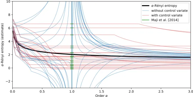
3.1 Estimates of α-Rényi entropy for varying values of α, computed on a syn-thetic geometric distribution with success probabilityq= 0.3, truncated to

{1,2, . . . ,500}and normalized. The exact value of the entropies is plotted in thick black. M = 30 sets of random perturbations have been sampled. For each set, the (Maji et al., 2014) estimate of the Shannon entropy is plotted atα= 1 in green, and the sample paths across varyingα of the normalized case Rényi entropy estimator (without the control variate, shown in blue) and with the control variate (Section 3.3.1, shown in red) are plotted. As predicted by Proposition 9 the latter sample paths pass through the (Maji et al., 2014) estimates at α= 1. . . 64

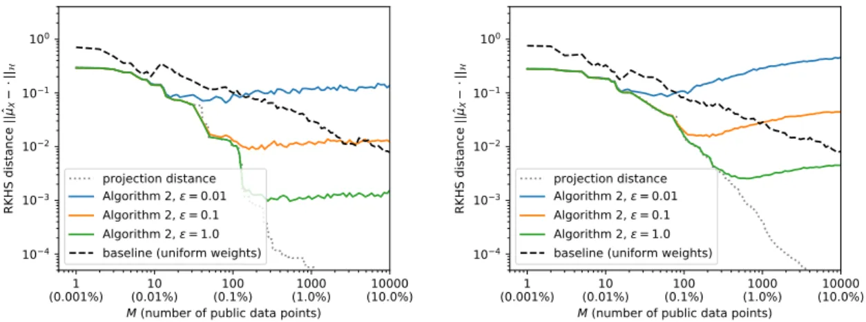
4.1 RKHS distance (lower is better) to the (private) empirical KME ˆµX computed

using the entire private database of size N = 100,000. The dimension of the database wasD= 2 (left) orD= 5 (right); please see Appendix C.2 for further details of the setup. Horizontally we variedM, the number of publicly releasable data points. Stricter privacy requirements (lowerε) naturally lead to lower accuracy. IncreasingM does not always necessarily improve accuracy, since a new public data point always increases the total amount of privatising noise that needs to be added, but this might not be outweighed by its positive contribution towards covering relevant parts of the input space. In all cases, for sufficiently smallM Algorithm 2 provided a more accurate estimate than

(15)

List of figures xv

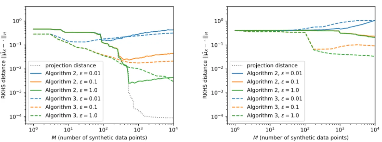
4.2 RKHS distance (lower is better) to the (private) empirical KME ˆµX computed

using the same databases as in Figure 4.1, of dimensionsD = 2 (left) and

D = 5 (right), but this time without a publishable subset. The synthetic data points for Algorithm 2 were therefore sampled from a wide Gaussian distribution; please see Appendix C.2 for further details. Algorithm 3 is capable of outperforming Algorithm 2 thanks to its ability to optimise the synthetic data point locations, but this depends on the precise optimisation procedure used and the optimisation problem becomes harder in higher dimensions. . . 83

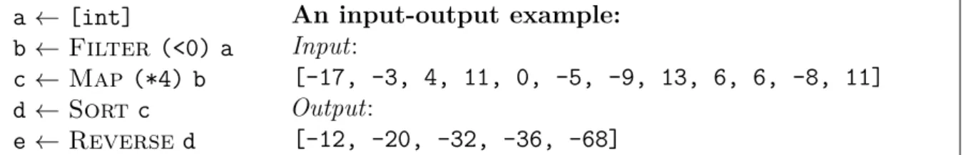
5.1 An example program in our DSL that takes a single integer array as its input. 95

5.2 Neural network predicts the probability of each function appearing in the source code. All instructions appearing in the ground truth program, shown in Figure 5.1, are correctly identified in this case. . . 97

5.3 (a) Search speedups on test programs of lengthT = 5. (b) Influence of length of training programs on the speedup. . . 100

D.1 Predictions of a neural network on the 9 example programs described in this section. Numbers in squares would ideally be close to 1 (function is present in the ground truth source code), whereas all other numbers should ideally be close to 0 (function is not needed). . . 164

D.2 Number of test problems solved versus computation time. . . 165

D.3 Number of test problems solved versus computation time. . . 166

D.4 Schematic representation of our feed-forward encoder, and the decoder. . . . 167

D.5 A learned embedding of integers {−256,−255, . . . ,−1,0,1, . . . ,255} in R2. The color intensity corresponds to the magnitude of the embedded integer. . 168

D.6 Conditional confusion matrix for the neural network and test set of P = 500 programs of length T = 3 that were used to obtain the results presented in Table 5.1. Each cell contains the average false positive probability (in larger font) and the number of test programs from which this average was computed (smaller font, in brackets). The color intensity of each cell’s shading corresponds to the magnitude of the average false positive probability. . . . 174

D.7 Conditional confusion matrix for the neural network and test set of P = 500 programs of length T = 5. The presentation is the same as in Figure D.6. . . 175

(16)

(17)

List of tables

2.1 New tricks for constructing unbiased estimators of different transformations

f(Z) of the partition function. The tricks are obtained by following the recipe of Section 2.2.2 and Example 6 with different choices of the functiong. See Section 2.2.3 for more details on the last column. . . 35

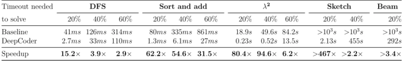
5.1 Search speedups on programs of length T = 3 due to using neural network predictions. . . 99

(18)

(19)

Chapter 1

Introduction

Machine learning has received an increasing amount of attention in recent years, partly

thanks to successful applications ofdeep learning(a subfield of machine learning, LeCun

et al., 2015) in disparate areas such as speech recognition (Hinton et al., 2012), computer vision (Krizhevsky et al., 2012), natural language understanding (Mikolov et al., 2013) and translation (Bahdanau et al., 2015), and many others. Breakthroughs in building autonomous agents for games such as Atari (Mnih et al., 2015), Go (Silver et al., 2016) and Starcraft (Vinyals et al., 2019) that match or even far surpass human performance have fuelled renewed interest in the aspiration of building “human-imitative” (Jordan, 2019) artificial intelligence (AI), to the extent that the terms AI and machine learning are nowadays sometimes conflated.

While some of the modern advances are due to the availability of larger datasets

and to the use of modern accelerator hardware such as GPUs (LeCun et al., 2015),

the aforementioned successes would not have been possible without having access to

methodology (principles, techniques, and algorithms) that had been developed many

years prior in a wide variety of fields including physics, mathematics, statistics, and computer science, and which continues to be developed to the present day.

This thesis is an attempt at usefully contributing to machine learning methodology, in the form of proposing new algorithms (new methods and generalizations of existing methods) for solving four important tasks. The thesis recognizes that most subtasks

encountered within machine learning fall into one of four categories – integration,

sampling,optimization, andsearch– and the common aspect of the proposed algorithms

is that they convert specificnon-optimization problems into optimization problems that

are in some sense easier to solve than the original problem. The four tasks addressed

(20)

of distributions, (2) the integration problem of estimating Rényi entropies, (3) the

sampling problem arising when wishing to release a database with sensitive data in a

differentially private manner, and (4) the search problem of automatic program source

code synthesis from an input-output example specification.

1.1

Non-technical Introduction

The purpose of this section is to explain the context and purpose of this thesis to a non-technical audience. It can be safely skipped by experts.

Machine learning Machine learning is a scientific field on the boundary of computer

science and statistics. It is concerned with computational methods that attempt to extract useful knowledge from data. A cartoon example of how this is different from classical computer science is provided by the following task:

Build an algorithm that can be shown an image containing an apple or a banana, and the algorithm responds with “apple” or “banana” depending on which of the two is actually in the picture.

A non-machine-learning approach would come up with rules that the computer

can use to distinguish apples from bananas, based on our human understanding of the differences between the two. For example, one might try using colour as such a distinguishing rule, classifying the image as containing a banana if it contains a group of yellow pixels next to each other. This can fail for a multitude of reasons, including the fact that apples can also be yellow, or the yellow group of pixels could simply be a table in the background. One might try to persevere and come up with better distinguishing rules such as trying to recognize whether there is a round (apple) or an elongated (banana) object in the picture, but again without a lot of care this can fail due to camera angles or other objects occluding part of the fruit’s shape. The point is that to build a reliable system in this way, one would have to:

1. think hard about the problem, and come up with more and more problem-specific

rules to cover different corner cases;

2. write computer code that implements the hand-designed rules. The more specific

a rule is to the problem at hand, the higher the chances that new complex computer code needs to be written (as opposed to reusing an already existing library).

(21)

1.1 Non-technical Introduction 3

As a result, this approach comes with a high human cost – both in terms of mental effort, and time spent developing new computer code.

The machine learning approach does away with much of this human cost, but the

price one needs to pay isdata. In our example, one needs to collect a dataset oflabelled

images of apples and bananas, i.e. a dataset where for each image it is known whether it contains an apple, or a banana. (This does not solve our task yet, because we still need to build an algorithm able to also classify images that are not part of this dataset.)

Supervised machine learning (currently the most widely applied subtype of machine

learning) essentially provides a generic recipe for automatically learning a classification rule that works well on the labelled dataset. If set up well, this rule can then be also

applied to images for which the answer is not yet known, in order to predict it.

Probability distributions Since machine learning algorithms are built to make

predictions about unknown quantities, the language of probability plays an important

role. A basic concept in probability is that of a probability distribution. As a common

example from the everyday world, a fair die defines a probability distribution that

places probability 1

6 on each of the numbers 1, 2, 3, 4, 5, 6. However, the distributions

encountered in machine learning can be much more complicated than that – think of an unfair die that is more likely to land on some side than others, and which instead of 6 sides has millions, or even an infinite number of sides it can land on.

Fundamental problems Most machine learning algorithms can be viewed as

con-sisting of one or more building blocks, where each block is solving one of the following four abstract, fundamental problems:

1. Integration: summing a large, or infinite list of numbers.

For example, estimating the sum of numbers written on each side of the die.

2. Sampling: obtaining a random sample from a given probability distribution.

For example, simulating a throw of the (possibly unfair) die.

3. Optimization: finding the maximum (highest point) of some function.

For example, finding the side of the die with the largest number.

4. Search: finding an element in a large set that satisfies some requirement.

(22)

Each of these tasks can be a very difficult problem in itself, generally because there are too many elements to sum up (in integration), to choose from (in sampling), or to consider (in optimization and search).

Conversions Remarkably, there are important cases where it is possible to “convert”

a problem of one of the four fundamental types into a problem of another type. For example, when wishing to sample from a probability distribution it is possible to convert the problem in such a way that instead it suffices to solve an optimization problem. Such ability to convert between different types of problems can be useful, for example because

• after conversion, the resulting new problem may have a special structure that can be exploited by specialized algorithms for the new problem;

• by performing a conversion, one can unlock new trade-offs: we will see an example where converting a sampling problem into an optimization problem allows trading off computation time for accuracy, which means that if one cannot afford to wait for the final result, it is possible to stop the algorithm early and extract a slightly less accurate but still useful answer.

This thesis contributes four new ways (or generalizations of previously known ways) to convert a specific non-optimization problem into an optimization problem.

1.2

Fundamental Problems

1.2.1

Optimization

Optimization refers to the general problem of finding an extremum (minimum or

maximum) of a scalar-valued functionf :X → _R∪ {−∞,∞}on some domainX. The

following notation is common, stated here for maximization:

f∗ = max

x∈X f(x), x

∗ _{= argmax}

x∈X

f(x). (1.1)

A primary differentiator of optimization problems, and the mathematical field of

(23)

1.2 Fundamental Problems 5

Discrete optimization On finite domains an optimization problem can be solved

trivially without any assumptions about f in O(|X |) steps by considering all domain

elements one by one. When |X | is prohibitively large or (countably) infinite,

assump-tions about f must be made, usually by relating its behaviour to an assumed structure

of X.

A type of structure particularly relevant for this thesis is a discrete graphical model,

representing the possible values ofn random variables in an undirected graphical model

(see also Section 1.5.1):

• the domain factorizes asX = X1×· · ·×Xn, where eachXirepresents the (discrete)

domain of variable i in the graphical model,

• a function f of interest is a potential function of the form f(x) = P

F∈FϕF(xF),

where F is a collection of subsets of the variables {1, . . . , n}, also called factors.

(The factors correspond to maximal cliques in the graphical model.)

The potential functionf of a graphical model defines its associatedGibbs probability

distribution p(x)∝exp (f(x)), and it’s easy to see that the problem of maximizing the

potential function f is equivalent to finding the maximum-probability configuration

under the Gibbs distribution. The latter problem is sometimes referred to as the MAP

(“maximum a posteriori”) problem, and it has been studied heavily in the literature (for example, Boykov et al., 2001; Kolmogorov, 2006; Sontag et al., 2008). The algorithms presented in Chapters 2 and 3 turn integration problems into this MAP problem and then exploit existing MAP solvers.

Other types of assumptions on the function being optimized can be made. One

important notion is submodularity, which ordinarily encodes the intuitive notion that a

non-negative set function has the “diminishing returns” property as more items are added into the set. In the context of discrete graphical models, a potential function

ϕF onXF :=Qi∈F Xi is submodular if

∀yF, zF ∈ XF ϕF(yF ∧zF) +ϕF(yF ∨zF)≤ϕF(yF) +ϕF(zF), (1.2)

where∧and∨respectively denote elementwise minima and elementwise maxima across

variables in the factor F. Making such submodularity assumptions can lead to faster

algorithms including to the MAP problem (Darbon, 2009). The algorithms presented in Chapters 2 and 3 have the property that they preserve submodularity properties of the discrete graphical model (if the original discrete graphical model is submodular, then so is the MAP problem generated by our conversion).

(24)

Continuous optimization Although “continuous” here refers to the domainX being

continuous, one also at the very least assumes continuity of f, lest the optimization

problem become hopeless. In most applications the function f is in fact assumed

differentiable (at least once, almost everywhere), and its gradient ∇f is used to inform

the optimization process (a first-order, or gradient-based optimization method). When

the function is twice differentiable and computing with its Hessian (matrix of second

derivatives) is computationally tractable, such second-order methods can be very

effective (Dennis Jr and Schnabel, 1996).

A main differentiator within the field of continuous optimization however, is whether

the function f is convex, or not. While convex optimization was arguably (and

incorrectly) considered solved in the 1980s (Jordan, 2018), non-convex optimization had been considered difficult. However, with revived interest in training (deep) neural networks whose training loss functions virtually always fail to be convex, non-convex optimization has gained prominence. Perhaps surprisingly, many techniques from convex optimization such as the simple stochastic gradient descent (SGD) or accelerated methods (Nesterov, 1983) have proven to be effective for training non-convex neural networks as well.

Chapter 5 casts the program synthesis search problem as a supervised learning task, and shows that it can be effectively tackled by training a neural network via standard (non-convex) gradient-based optimization.

Bayesian optimization Although Bayesian optimization (Brochu et al., 2010;

Shahriari et al., 2015) is a method for both discrete and continuous optimization

problems, we mention it here separately thanks to its focus on optimizing expensive-to-evaluate black-box functions, often without access to its derivatives. In the discrete

case this corresponds to thebest arm identification problem (orpure explorationsetting)

inMulti-Armed Bandits (MAB, Bubeck et al., 2009).

Chen and Ghahramani (2016) showed how to convert a large-scale sampling problem

into such a MAB problem using the Gumbel trick, and we also use this large-scale

setup in Section 2.5.2 to evaluate our new methods for partition function estimation.

1.2.2

Integration

In this thesis, an integration problem is the task of evaluating adefinite integral

I :=

Z

A

(25)

of a real-valued function f : A → _R with respect to some measure µ on A. This

includes summation problems P

x∈Af(x) on discrete domains A by taking µto be the

counting measure on A. However, note that this is different from symbolic integration,

as we do not require that f has a closed-form anti-derivative.

Two primary sources of integration problems in machine learning are the needs of (1) computing normalizing constants of unnormalized distributions, and (2) evaluating

expectations with respect to specific distributions.

Example 1 (Normalizing constants). In an undirected graphical model (see also

Section 1.5.1), the joint probability distribution is specified by a potential (negative

energy) function ϕ : X → [−∞,∞) through p(x) ∝ exp(ϕ(x)). Computing actual

probabilities requires obtaining the normalizing constant Z := R

xexp(ϕ(x)) dx, which

is also called the partition function in this context and its estimation will be the focus

of Chapter 2.

Example 2 (Evaluating expectations). After computing a Bayesian posterior of

model parameters p(θ|x) given observed data x, one may wish to report the findings

by providing scalar summaries, such as expected values of θ-dependent quantities

(perhaps E[θ] itself).

Example 3 (Entropy estimation). An important property of any probability

distri-bution is the amount of uncertainty it encodes, which can be quantified by various

measures of entropy. The Shannon entropy of a discrete distribution p is given by

H1(p) :=−Pxp(x) lnp(x) and the Rényi entropy with parameter α∈(0,1)∪(1,∞)

is given by Hα(p) := ₁₋1_αlnPxp(x)α. Note that the former can be written as the

expectation Ep[−lnp(x)] with respect to the distributionp. The Rényi entropy can

be expressed as a transformed expectation Hα(p) = ₁₋1_αlnEp[p(x)α−1], which will be

exploited in Chapter 3. See also Section 1.5.2 for important special cases of Rényi entropies.

Perhaps the most common type of integration problem in Bayesian machine learning is in fact both a normalizing constant evaluation problem, as well as an expectation evaluation problem. After application of Bayes theorem to compute a posterior distribution of interest, p(θ|x) = p(x,θ) p(x) = p(x|θ)p(θ) R θp(x|θ)p(θ) dθ , (1.4)

(26)

the denominator (calledmodel evidence) is both the normalizer of the joint distribution

p(x,θ) in the numerator, as well as the integral of the likelihoodp(x|θ) with respect

to the prior p(θ).

The model evidence is useful for (Bayesian) model selection when multiple models are under consideration. In particular, the ratio between two model evidences is called

aBayes factor and can be used to compare two competing model hypotheses. The term

marginal likelihood is sometimes also used to refer to the model evidence, especially

when θ are latent (nuisance) variables, to be marginalized out. Optimizing the

marginal likelihood across a space of models indexed by continuous model parameters is sometimes called model learning.

More generally, any marginalization problem of computing a distribution of a

set of variables yA from a joint distribution of yA and yB, leads to this type of

integration problem. Similarly, any type of probabilistic conditioning leads to such a marginalization and thus integration problem through the definition of conditional probability.

Example 4 (Counting problems). In a counting problem one wishes to count the

number of elements in a larger set Ω satisfying a given predicate P : Ω → {true,false}.

This can also be seen as an integration problem by integrating the indicator function

1P of the predicate with respect to the counting measure on Ω. Valiant (1979) defined

the #P computational complexity class, comprising of counting problems where the

predicateP can be evaluated in polynomial time. For example, the problem of counting

the number of satisfying assignments to a given propositional formula is in #P. Note that counting problems in #P are at least as hard as their corresponding decision problems in NP, because it suffices to check whether the count is non-zero in order to solve the decision problem. In fact, the class #P is believed (but not proved) to be strictly harder than NP.

1.2.3

Sampling

A widespread use of sampling in machine learning is to perform Monte Carlo estimation

of expectations, which is in fact a prime example of a conversion from anintegration

problem to sampling and will be discussed in Section 1.4.2. However, there are

interesting and important cases where the randomness provided by sampling is useful

(27)

Stochastic gradient methods In supervised machine learning one tends to

mini-mize the (regularized) empirical risk on the training data, and if the empirical risk is differentiable – as it is with, say, most neural networks – gradient-based optimization methods are employed. However, instead of utilizing the exact gradient computed across the full training data, often one only considers a noisy version of it in each

iteration by subsampling the training data (mini-batch gradient descent); in the extreme

case of stochastic gradient descent (Robbins and Monro, 1951) the gradient is computed

on a single, randomly chosen training data point.

However, the benefit of stochastic gradient methods lies not only in the computa-tional cheapness of computing mini-batch gradients; there are also theoretical reasons to prefer them over full-batch methods (Bottou et al., 2018). Moreover, the noise present in the stochastic gradient is useful for finding minima of neural network loss landscapes that have better generalization properties (Dziugaite and Roy, 2017; LeCun et al., 2012).

In the i.i.d. setting this sampling problem is straightforward computationally, as one only needs to sample uniformly from a set of tractable size (the number of data points).

In Chapter 5 we use a more sophisticated variant of SGD calledAdam (Kingma

and Ba, 2015) to perform gradient-based optimization of a neural network in order to speed up a discrete search problem.

Differential privacy As machine learning solutions permeate everyday life, the

question of individual privacy is gaining importance. On one hand, it has been shown that one can extract private information about training data points from a trained neural network (Fredrikson et al., 2015). On the other hand, in areas such as medicine strict regulations governing the use of individual data are already in place, but the ability to (safely) apply machine learning approaches could lead to substantial leaps in healthcare; e.g., better personalized treatment or cohort identification for clinical trials (Dankar and El Emam, 2013).

Differential privacy (Dwork, 2006) has emerged as the leading formalization of

privacy that allows individuals to share their data in a way that allows quantifying how much privacy they lose by doing so. The main idea behind differentially private

algorithms is that of addition of noise, which provides a form of plausible deniability to

the participating individuals (Dwork and Roth, 2014), as illustrated by the following cartoon example.

(28)

Example 5 (Randomized response). Suppose you want to find out the proportion

of people in a conference room that have tried narcotics in their life. Asking those who have to raise their hand may underestimate the true value due to reluctance towards admitting such behaviour. However, as the conductor of the experiment you could first ask each person to discreetly throw a coin twice and remember the two results. If the first throw landed heads, they should answer your question truthfully, and otherwise they should randomize their answer according to the second coin toss.

This way, anyone raising their hand now has plausible deniability, but the fraction of

raised hands can still be used to estimate the true ratio with useful accuracy (Dwork and Roth, 2014). Moreover, by replacing fair coin tosses with biased ones it is possible to trade-off between the accuracy of this estimate and the privacy violation incurred by each participant.

In Chapter 4 we consider the problem of publicly releasing an entire database

containing sensitive data, also known as offline differential privacy. To protect the

privacy of the data, the released dataset will be a noisy version of the original database.

A canonical algorithm for computing such a noised database, called SmallDB (Blum

et al., 2008), requires sampling a synthetic database from a specific distribution supported on the set of all possible databases (with the same schema and size), which is computationally intractable for all but the simplest cases. Chapter 4 shows how the problem can be approached from a perspective of Reproducing Kernel Hilbert Spaces

and then converted into an optimization problem.

Exploration algorithms Inbandit optimization (Bubeck et al., 2009) and

reinforce-ment learning (RL, Sutton and Barto, 1998) an agent interacts with an environment

and receives rewards. Since the distribution of rewards (and in the case of RL also

the dynamics of the environment) are unknown to the agent, it needs to explore the

environment to discover areas with high reward. Randomized exploration strategies have been shown to be effective for achieving this goal. A well-known example is Thompson sampling (Thompson, 1933) where one point is drawn from the distribution encoding current beliefs of the agent about its environment, and the next action is optimized with respect to this one sample. Thompson sampling also forms basis of posterior sampling reinforcement learning (PSRL, Dearden et al., 1998), an exploration strategy in RL.

Bandit optimization problems can also arise artificially; for example, Chen and Ghahramani (2016) cast a large-scale discrete sampling problem as a bandit optimization

(29)

problem using the Gumbel trick. We adapt this setup to partition function estimation

and use it to evaluate our new generalizations of the Gumbel trick in Section 2.5.2.

Other randomized algorithms Sampling is generally required in all randomized

algorithms. A specific problem type where randomized algorithms can be useful are

adversarial setups, where an online algorithm operates against an adaptive adversary

whose actions can depend on previous decisions of the algorithm. Intuitively, ran-domization is helpful because the adversary at least cannot know the next action of

the algorithm. For example, the paging problem is the problem of deciding which

documents to keep in a fast cache of limited size in order to minimize the total number of future cache misses. Fiat et al. (1991) showed that a randomized algorithm can achieve a strictly better competitive ratio against the best possible offline algorithm than any deterministic algorithm could.

1.2.4

Search

Classical AI “Classical” artificial intelligence (Russell and Norvig, 2016) as pursued

since the 1950s has focused on techniques using explicit knowledge representations, logical reasoning, and planning. Examples of common problem formalizations were graph problems, constraint satisfaction problems (CSPs), and games. These problems were addressed through discrete or continuous search algorithms, a basic but well-known

example of which is A∗ search (Hart et al., 1968).

Program synthesis Even as researchers aspiring to development of artificial

in-telligence increasingly look towards statistical techniques, search problems are still present in the machine learning domain. In fact, some believe that a key stepping

stone towards building intelligent agents can be achieved through progress in program

synthesis (Goodman et al., 2014, Section 7), and indeed program synthesis has been

considered a “holy grail of computer science” (Gulwani et al., 2017). In program synthesis the task is to automatically construct program source code from a given specification, such as input-output examples. The high-level idea is that an agent released in an unknown environment should be able to learn the laws governing said environment from interactions (inputs) and observations (outputs) in order to be able to plan its future actions (Reed and De Freitas, 2016). While a similar goal is pursued

(30)

learns a program implicitly in its trainable weights, learning an explicit program has several advantages:

1. a restricted programming language or a preference for shorter programs can

encode the usefulinductive bias towards simpler laws of the world,

2. a program is interpretable by a human and can be assessed for correctness, and

3. it can be further modified and composed in transparent ways.

In fact, in recent years there has been renewed interest in combining symbolic reasoning approaches with learning based systems in a symbiotic manner. An early example of

this type of modern neuro-symbolic approach is the work on guiding program synthesis

search using a trained neural network, which will be presented in Chapter 5.

Automated theorem proving A related area to program synthesis is that of

automated theorem proving, where the task is to automatically construct proofs of a

given mathematical statement by suitably combining a (large) set of given axioms and lemmas. Similarly to program synthesis, approaches that combine symbolic search with neural networks have been pursued (Alemi et al., 2016).

1.2.5

Conversions

Reductions and conversions Theoretical computer science and in particular the

study of formal models of computation and complexity theory rely heavily on the

(31)

1.3 Conversions 13

problem into another. A reduction f from a problem A to another problem B is

useful because it shows that the problem A is computationally no harder than the

combined computational complexity of problem B and of computing the reduction

f. For example, a Turing reduction (an arbitrary computable function) from an

undecidable problem Ato another problem B proves that the latter is also undecidable.

Similarly, apolynomial-time reduction from an NP-hard problemAto another problem

B proves that the latter is also NP-hard.

This thesis focuses on problem transformations that translate between different types of abstract fundamental problems discussed in the preceding Section 1.2. However, they

are not necessarilyreductions in the formal sense, because in some cases the application

permits that the solution after applying the transformation is only approximate, or that solving the transformed problem requires an additional resource type (such as data).

Hence, to avoid confusion, in this thesis we will use the term conversion (instead of

reduction) to describe the problem transformations considered. However, they do share with formal reductions the notion of efficient computability, as we seek conversions that are practically applicable.

Why conversions? A natural question to ask is why one should consider converting

between different problem types at all, if one is interested in solving them rather than proving hardness results. Why is it not simpler to construct a solution within the original problem type? Indeed, as expected we shall see that none of the existing conversions discussed later in Section 1.4 are a silver bullet that would provide a general performance gain on its own. However, the following list shows broad categories of situations where a conversion to a different problem type can be beneficial (the first three points are closely related to each other). After the high-level list, the specific examples of the four conversions studied in this thesis are categorized. Section 1.4 then provides more examples of existing useful conversions within the field of machine learning.

• Historical development

Although all of optimization, integration, sampling andsearch are well-studied

problems, none is considered completely solved, and researchers working on each of these problems have had different perspectives, motivations, and backgrounds, leading to some sub-types of these problem classes being better explored than others. As a result, converting into a different problem type might map onto a specific problem instance that has been more thoroughly studied.

(32)

• Well-studied problem structure

The Gumbel trick and its generalizations presented in Chapters 2 and 3 not only map onto the well-studied problem of finding the most likely configuration in a discrete graphical model (an example of the previous point), the conversion is such that it preserves submodularity properties of the discrete graphical model, and as such makes it amenable to fast MAP solvers in common cases.

• Effectiveness of heuristics

The previous two points are especially relevant for heuristics, as different fields have developed their own set of heuristics following their applications of interest.

• Unlocking new trade-offs

When designing machine learning solutions, one needs to take multiple types of costs and constraints into account. Apart from the typical notions of (1) computation time and (2) space (memory) that are ubiquitous in computer science, these are also (3) sample (data) complexity, (4) statistical risk, (5) privacy, (6) fairness, and possibly others. Converting to a different problem type can unlock different types of trade-offs between these quantities.

• Implementation advantages and convenience

Converting into a different problem type could also be done for convenience or availability of robust implementations. For example, when wishing to sample from a trained RNN decoder outputting logits (unnormalized log probabilities), a convenient way is to utilize the Gumbel trick, which in this case has the same time and memory complexity as standard sampling but it is simpler to implement and numerically more stable, because it does not require normalization of probabilities and instead acts directly on the logits.

• New understanding

Finally, converting to a different problem type can lead to a better understanding of the original problem. For example, rephrasing a problem as an optimization problem using duality or the variational framework more generally, one can consider perturbations of the derived optimization problem and study how they affect the resulting solution (Jordan et al., 1999).

The conversions studied in this thesis tend to fall into multiple categories:

• The Gumbel trick (Papandreou and Yuille, 2011) and its generalizations presented in Chapters 2 and 3 convert integration problems to the well-studied optimization

(33)

1.4 Examples of Conversions in Machine Learning 15

problem of finding the MAP (most likely) configuration in a discrete graphical model. However, they also introduce a new type of trade-off between computation time and statistical accuracy, as they lead to stochastic approximation schemes. • The work on differentially private database release via kernel mean embeddings

presented in Chapter 4 yields an optimization algorithm with theanytimeproperty

and thus introduces a new trade-off between computation time and accuracy. The

original sampling problem would have a trade-off between computation time and

privacy, which would be useless if one wants to guarantee that a certain privacy level is attained (which is indeed the point of differential privacy). Moreover, the

conversion allows utilizing any optimization heuristics on the generated reduced

set optimization problem (Schölkopf and Smola, 2002, Chapter 18).

• In Chapter 5, casting the discrete search in program synthesis as a supervised learning task that can be solved using neural networks unlocks the ability to exploit the efficiency of gradient-based optimization of neural network models (which one might consider a heuristic for minimizing non-convex loss functions)

in order to solve an inherently discrete problem.

1.4

Examples of Conversions in Machine Learning

1.4.1

Conversions to Optimization Problems

Variational inference Variational methods, historically derived from the field of

calculus of variations (Lagrange, 1788), have entered machine learning through mean

field methods from statistical physics (Parisi, 1988). Variational methods have turned

out to be very successful within the formalism of graphical models (Jordan et al., 1999; Wainwright and Jordan, 2008), where they provide a powerful paradigm for approximate

(variational) inferenceby rewriting anintegration problem into anoptimizationproblem.

In modern probabilistic machine learning one often posits a generative model

involving observed variables x (the data), latent variables z (to be inferred), and

model parameters θ (to be learned). The generative distribution can be described by a

directed graphical model, with edges indicating probabilistic dependencies (conditional probability distributions). With such a probabilistic formulation it is natural to take, at least partially, a Bayesian approach and work with posterior distributions

(34)

commonly required operations such as sampling, marginalization, and evaluating

expectations (both examples of integration problems) under posterior distributions can

be computationally intractable, especially when there is a large number of unobserved variables (Zhang et al., 2018).

Variational inference (Blei et al., 2017) takes the approach of defining a variational

family of probability distributions Q = {qλ : λ ∈ Λ}, parametrized by variational

parameters λ, such that (1) required operations are tractable for distributions inQ, (2)

Qis rich enough to approximate the posterior distribution of interest sufficiently well,

and (3) optimization overQ (or Λ) is tractable. The algorithmic crux of variational

inference is then to solve the optimization problem

q∗ ←argmin

q∈Q

D(p, q) =qargminλ∈ΛD(p,qλ), (1.5)

where p is the posterior of interest, and D(p, q) is a divergence measure between

distributions p and q (a non-negative function that equals 0 if and only if p = q).

The most common choice is the reverse Kullback-Leibler (KL) divergence D(p, q) =

KL(q∥p) = R

qlnp_q, although other choices including Rényi α-divergences have also

been explored (Li and Turner, 2016).

Graph message passing algorithms (Loopy) belief propagation (Murphy et al.,

1999; Pearl, 1988) andExpectation maximization (EP) (Minka, 2001) are two examples

of approximate inference methods for graphical models that can be interpreted on one hand as (1) message passing algorithms on the graph, but also as (2) solving an optimization problem (although with EP the situation is more subtle, Bui et al., 2016). Wainwright and Jordan (2008) thus argued that these methods should be seen as part of the variational methods family, because they involve an optimization to approximate a density of interest.

Perturb-and-MAP Perturb-and-MAP methods (Papandreou and Yuille, 2011)

con-stitute a class of randomized algorithms for converting the sampling problem, and

the problem of estimating normalizing constants (an integration problem) into the

optimization problem of finding a highest-probability configuration. The algorithms

operate by first randomly perturbing the target probability distribution and then employing maximum a posteriori (MAP) solvers on the perturbed models to find a maximum probability configuration, hence the name of the framework. As the

(35)

1.4 Examples of Conversions in Machine Learning 17

random perturbations involve the Gumbel distribution (Gumbel, 1935), the framework

is sometimes also described as (utilizing) the Gumbel trick.

More specifically, Papandreou and Yuille (2011) first introduced the framework in

the context of discrete graphical models. Given a potential function ϕ :X → [−∞,∞)

defining the Gibbs distribution p(x)∝exp(ϕ(x)) on a finite state space X, the problem

of sampling p can be approached by adding an independent Gumbel perturbation to

each configuration’s potential, and then finding the highest-potential configuration. Hazan and Jaakkola (2012) pointed out that such perturbations are useful not only

for sampling the Gibbs distribution (considering the argmax of the perturbed model),

but also for bounding and approximating the normalizing constant (by considering the

value of the max), which is also known as thepartition function in this context. Later,

Maji et al. (2014) exploited the duality relationship between the partition function and the Shannon entropy to construct perturb-and-MAP estimators of this entropy.

Although the resulting MAP problems are NP-hard in general, substantial research effort has led to the development of solvers which can efficiently compute or estimate the MAP solution on many problems that occur in practice (e.g., Boykov et al., 2001; Darbon, 2009; Kolmogorov, 2006). Evaluating the partition function is a harder problem, containing #P-hard counting problems.

Specific instances of the Perturb-and-MAP framework and their applications are described in more detail in Section 2.1. Chapter 2 also introduces a generalization

of the Gumbel trick to a wider family of algorithms utilizing different perturbation

distributions, some of which have more favourable statistical properties when estimating normalizing constants. Chapter 3 presents an extension of the Gumbel trick (and

also of the new tricks from Chapter 2) to a new integration problem, the problem of

estimating Rényi entropies.

Other partition function estimators via MAP calls Other methods that

es-timate the partition function of a discrete graphical model via MAP solver calls include:

• The WISH method (weighted-integrals-and-sums-by-hashing, Ermon et al., 2013) relies on repeated MAP inference calls applied to the model after subjecting it to random hash constraints.

• The Frank-Wolfe method may be applied by iteratively updating marginals using a constrained MAP solver and line search (Belanger et al., 2013; Krishnan et al., 2015).

(36)

• Weller and Jebara (2014a) used a single MAP call over a discretized mesh of marginals to approximate the Bethe partition function, which itself is an estimate of the true partition function.

Search by optimization Suppose one wants to find an element x∈ X on a (finite

or infinite) search space X satisfying a predicate P : Ω → {true,false}. One can

trivially set up a maximization optimization problem x∗ ←argmax_x∈X1P(x) that is

computationally equivalent to the original search problem. Naturally, such a refor-mulation is not useful on its own, but can be made such through a relaxation – for

example, replacing 1P(x) with a smoother (e.g., differentiable) function Q:X →[0,1]

that approximates 1P. The work presented in Chapter 5 can be seen as an instance

of this general approach, because a neural network is trained to make probabilistic predictions about properties of the solution that is being searched for, and thus induces

a functionQ on the search space of programs X that approximates the indicator₁P of

the predicate P.

Another type of relaxation is when the space X itself is extended, such as whenX

is discrete but Q can be defined on a larger X′

⫌X such that Q(x) is close to 1P(x)

on X, andQ is continuous on X′_{. An instance of this is a search problem encoded as}

an integer programming problem, which is in turn relaxed to linear programming by elimination of integrality constraints on the variables.

1.4.2

Conversions in Other Directions

Although not a focus of this thesis, for completeness we provide three important examples of conversions between fundamental problems that do not reduce to an optimization problem, but instead go in different directions.

Integration to sampling Perhaps the most widely known conversion technique

of all is that of Monte Carlo sampling, where the integration problem of evaluating

a definite integral I := R

f(x)p(x) dx with respect to a probability density p(x) is

converted into the problem of sampling points x1, . . . , xN from p or an approximation

thereof such that the quantity of interest can be approximated by ˆI := 1

N

PN

n=1f(xn).

Optimization to sampling Suppose one wishes to minimize a function f :X →_R.

One can set up the problem of sampling a probability distribution pon X with density

(37)

1.5 Tasks Considered in This Thesis 19

Asβ is annealed to∞, samples frompβ(x) will concentrate towards minima off. This

classical technique is called simulated annealing.

Sampling to integration Sampling a structured probability distributionp(x1, . . . , xn)

onX =X1× · · · × Xn, such as a discrete graphical model, can be performed much faster

if one can efficiently solve integration problems of evaluating marginals (and

condition-als). Specifically, one can sample X1 from the marginal distribution of p(x1) and then

for each i= 2, . . . , n sample Xi from the conditional distribution p(xi |x1, . . . , xi−1).

This brings down the computational complexity of sampling fromO(|X |) (exponential

in n) to O(nmaxi|Xi|) (linear in n). A conversion of this type is used by Hazan et al.

(2013) in the Perturb-and-MAP framework, and also by us in Section 2.3.3.

1.5

Tasks Considered in This Thesis

This section introduces the specific tasks for which subsequent chapters of the thesis present beneficial conversions to optimization problems.

1.5.1

Estimating Normalizing Constants

Given an unnormalized probability distribution, i.e. an unnormalized probability mass function in the discrete case or an unnormalized density function in the continuous case,

denoted by ˜p:X → [0,∞), the task is to compute the normalization constantZ := R

Xp˜

(which corresponds to the summationZ :=P

x∈Xp˜(x) in the discrete case by considering

the counting measure on X). Section 1.2.2 outlined how this integration problem

commonly arises in machine learning applications involving undirected graphical models, Bayesian modelling, and marginalization or conditioning of probability distributions more generally; these are all fundamental tools with ubiquitous applications.

Undirected graphical models The case of estimating normalizing constants of an

undirected graphical model will be of particular interest in Chapter 2 and Section 2.3

more specifically. Given an undirected graph G= (V, E) where the vertices V index

random variables X = {Xv | v ∈ V} taking values in X = Qv∈V Xv, an undirected

(38)

over X that factorizes along the cliques (maximal fully-connected subgraphs) of G: p(x) = 1 Z Y C⊆V a clique ψC(xC), (x∈ X). (1.6)

HerexC :={xv |v ∈C}andψC :Qv∈CXv →[0,∞) describes the mutual compatibility

of assignments to random variables in the clique C. In this context, the scalar

normalizing constantZ is called thepartition function. The term comes from statistical

physics, where the partition function describes how probability mass is partitioned among possible microstates of a system depending on their energies. The non-negative

compatibility functions ψC can always be rewritten in exponential form to reveal what

is called a Gibbs distribution, or in finite-variable cases also theBoltzmann distribution:

p(x) = 1 Z Y C⊆V a clique ψC(xC) = 1 Z exp     X C⊆V a clique ϕC(xC)    = 1 Z exp     − X C⊆V a clique EC(xC)     . (1.7)

Here ϕ is called the potential function, and E the energy; they are related simply by a

sign change. Chapters 2 and 3 will be phrased in terms of the potential functionϕ(x) :=

P

CϕC(xC), which one can recognize as simply the logarithm of the unnormalized

probability mass or density function: ϕ(x) = ln(Zp(x)).

Discrete graphical models The framework of undirected graphical models permits

both discrete and continuous random variables, or indeed a combination thereof. Although the continuous case will be considered in Section 2.5.1, our focus will be on

the setting where all random variables Xi take values in finite sets Xi, in which case

we talk about discrete graphical models.

A canonical example of a discrete graphical model is an Ising model (Lenz, 1920),

again from statistical physics. It models a system of magnetic atoms, where each

can have a positive or negative spin: the variable Xi represents the spin of atom

i and takes values in {−1,+1}. Edges of the graphical model link adjacent atoms,

encoding that there is an interaction between them. In the case of an Ising model the edges usually form a 2D or 3D lattice, and consequently all cliques consist of

just two vertices joined by an edge. The potential function thus consists ofpairwise

potentials: ϕ(x) = P

e∈Eϕe(xe). Extensions include the addition of an external

(39)

1.5 Tasks Considered in This Thesis 21

and the generalization to more than two spins, which is then called aPotts model (Potts,

1952).

Apart from widespread use in statistical physics, applications of discrete graphical models in machine learning include Hopfield networks (Little, 1974) for simulating an associative memory, and the general class of Boltzmann machines (Ackley et al., 1985) including Restricted Boltzmann machines (RBM, Smolensky, 1986) and Deep Boltzmann machines (DBM, Salakhutdinov and Hinton, 2009) whose addition of hidden units (with values not observed during training) permits representation learning and have been used for tasks such as collaborative filtering (Salakhutdinov et al., 2007), classification (Larochelle and Bengio, 2008) and sequence modelling (Sutskever and Hinton, 2007).

Computing the partition function of a discrete graphical model is in general equiva-lent to computing a matrix permanent, which is a #P-hard problem (Valiant, 1979), a computational complexity class that is believed to be even harder than NP.

1.5.2

Rényi Entropy Estimation

Entropies are measures of uncertainty in a probability distribution. The most commonly

used is the Shannon entropy (Shannon, 1948), defined by H1(p) :=Px∈Xp(x) lnp(x).

The Shannon entropy possesses strong information-theoretic properties and its esti-mation has found a wide array of applications within statistics (Goria et al., 2005), machine learning (Learned-Miller and John III, 2003), as well as other fields (Porta et al., 2001).

The Rényi entropy (Rényi, 1960) can be seen as a generalization of the Shannon

entropy into a continuous class of entropies parametrized by α ∈ [0,∞]. For α ∈

(0,1)∪(1,∞) the α-Rényi entropy is given by Hα(p) := ₁−1αln

P

x∈Xp(x)α, and it is

extended to the boundary values via appropriate limits. This definition encompasses and generalizes multiple measures of uncertainty with important roles in different fields:

• α= 0 is the Hartley entropy, related to the distribution’s support size;

• α= 1 is the Shannon entropy, the most widely used entropy measure;

• α= 2 is the collision entropy, equal to the negative logarithm of the probability

that two independent draws from the distribution coincide;

(40)

Section 3.2.1 provides more information on particular α-Rényi entropies.

Literature on entropy estimation usually assumes access toN samplesx1, . . . , xN

iid

∼

p from the unknown distribution p, and the task is to estimate the entropy of p

from these N points. In the perturb-and-MAP framework no samples from p are

assumed; instead, the distribution of interest is described by a potential function

ϕ:X → [−∞,∞), as in Section 1.5.1. Computing the entropy remains a challenging

problem in this setting because it amounts to computing an integral over the support of

p. Maji et al. (2014) exploited the duality relationship between the partition function

and the Shannon entropy to construct a perturb-and-MAP estimator of the Shannon entropy based on the Gumbel trick. Chapter 3 shows how the perturb-and-MAP framework (including both the Gumbel trick and the new tricks from Chapter 2) can be cleanly extended to the integration problem of estimating Rényi entropies. The relationship with the existing estimator of the Shannon entropy due to Maji et al. (2014) is also discussed in detail.

1.5.3

Differentially Private Database Release

In Chapter 4 we are concerned with the following problem. Given a database of records containing sensitive data (e.g., patient health records), the trustworthy curator of this database wishes to releas