MPRA
Munich Personal RePEc Archive
Credit Cycles, Credit Risk, and
Prudential Regulation
Jesus, Saurina and Gabriel, Jimenez
20. March 2006
Online at
http://mpra.ub.uni-muenchen.de/718/
Prudential Regulation
∗Gabriel Jim´enez and Jes´us Saurina
Banco de Espa˜na
This paper finds strong empirical support of a positive, although quite lagged, relationship between rapid credit growth and loan losses. Moreover, it contains empirical evidence of more lenient credit standards during boom periods, both in terms of screening of borrowers and in collateral requirements. We find robust evidence that during upturns, riskier borrowers get bank loans, while collateralized loans decrease. We develop a regulatory prudential tool, based on a countercyclical, or forward-looking, loan loss provision that takes into account the credit risk profile of banks’ loan portfolios along the busi-ness cycle. Such a provision might contribute to reinforce the soundness and the stability of banking systems.
JEL Codes: E32, G18, G21.
∗This paper is the sole responsibility of its authors, and the views represented
here do not necessarily reflect those of the Banco de Espa˜na. We thank R. Repullo
and J. M. Rold´an for very fruitful and lively discussions about prudential banking
supervisory devices. We are also grateful for the detailed comments provided by V. Salas; H. Shin, the editor; J. Segura; an anonymous referee; and participants at the BCBS/Oesterreichische Nationalbank Workshop; the Bank of England
work-shop on the relationship between financial and monetary stability; X Reuni´on
de la Red de Investigadores de Bancos Centrales Iberoamericanos in Per´u; XX
Jornadas Anuales de Econom´ıa in Uruguay; Foro de Finanzas in Madrid; and FUNCAS Workshop Basilea II y cajas de ahorros in Alicante. In particular, we
would like to express our gratitude for the comments of S. Carb´o, X. Freixas,
M. Gordy, A. Haldane, P. Hartman, N. Kiyotaki, M. Kwast, M. Larra´ın, J. A. Licandro, I. van Lelyveld, P. Lowe, L. A. Medrano, J. Moore, C. Tsatsaronis, and B. Vale. Any errors that remain are entirely the authors’ own.
Correspond-ing author: Saurina: C/Alcal´a 48, 28014 Madrid, Spain; Tel +34-91-338-5080;
e-mail: jsaurina@bde.es.
1. Introduction
Banking supervisors, after many painful experiences, are quite con-vinced that banks’ lending mistakes are more prevalent during
upturns than in the midst of a recession.1 In good times both
bor-rowers and lenders are overconfident about investment projects and their ability to repay and to recoup their loans and the corresponding fees and interest rates. Banks’ overoptimism about borrowers’ future prospects, coupled with strong balance sheets (i.e., capital well above minimum requirements) and increasing competition, brings about
more liberal credit policies with lower credit standards.2Thus, banks
sometimes finance negative net present value (NPV) projects only to find later that the loan becomes impaired or the borrower defaults. On the other hand, during recessions—when banks are flooded with nonperforming loans, high specific provisions, and tighter capital buffers—banks suddenly turn very conservative and tighten credit standards well beyond positive net present values. Only their best borrowers get new funds; thus, lending during downturns is safer and credit policy mistakes much lower. Across many jurisdictions and at different points in time, bank managers seem to overweight concerns regarding type 1 lending policy errors (i.e., good borrowers not getting a loan) during economic booms and underweight type 2 errors (i.e., bad borrowers getting financed). The opposite happens during recessions.
Several explanations have appeared in the literature to rational-ize fluctuations in credit policies. First of all, the classic principal-agency problem between bank shareholders and managers can feed excessive volatility into loan growth rates. Once managers obtain a reasonable return on equity for their shareholders, they may engage in other activities that depart from the firm’s value maximization and focus more on their own rewards. One of these activities might be excessive credit growth in order to increase the social presence of the bank (and its managers) or the power of managers in a con-tinuously enlarging organization (Williamson 1963). If managers are
1
See, for instance, Caruana (2002), Ferguson (2004), and the numerous joint announcements by U.S. bank regulators in the late nineties warning U.S. banks to tighten credit standards.
2A loose monetary policy can also contribute to overoptimism through excess
rewarded more in terms of growth objectives instead of profitability targets, incentives to rapid growth may result. This has been doc-umented previously by the expense preference literature and, more
recently, by the literature that relates risk and managers’ incentives.3
Strong competition among banks or between banks and other financial intermediaries erodes margins as both loan and deposit interest rates get closer to the interbank rate. To compensate for the fall in profitability, bank managers might increase loan growth at the expense of the (future) quality of their loan portfolios. Excess capacity in the banking industry is being built up. Nevertheless, that will not impact immediately on problem loans, so it might encourage further loan growth.
In a more formalized framework, Van den Heuvel (2002) shows that the combination of risk-based capital requirements, an imper-fect market for bank equity, and a maturity mismatch in banks’ balance sheets gives rise to a bank capital channel of monetary pol-icy. In boom periods, when banks show strong balance sheets and capital buffers, they overlend. However, as the expansion heads to its end, the surge in loan portfolios has eroded much of the capital buffer; at that point, a monetary shock may trigger a decline in bank profits, stringent capital ratios, and a tightening of lending standards
and, subsequently, of loans available to firms and households.4
Herd behavior (Rajan 1994) might also help to explain why bank managers finance negative NPV projects during expansions. Credit mistakes are judged more leniently if they are common to the whole industry. Moreover, a manager whose bank systematically loses mar-ket share and underperforms its competitors in terms of earnings growth increases his or her probability of being fired. Thus, managers have a strong incentive to behave as their peers, which, at an aggre-gate level, enhances lending booms and recessions. Short-term objec-tives are prevalent and might explain why banks finance projects during expansions that, later on, will become nonperforming loans. Berger and Udell (2004) have developed the so-called institu-tional memory hypothesis in order to explain the markedly cyclical
3For the former, see (among others) Edwards (1977), Hannan and Mavinga
(1980), Akella and Greenbaum (1988), and Mester (1989). For the latter, see Saunders, Strock, and Travlos (1990), Gorton and Rosen (1995), and Esty (1997).
4
Ayuso, P´erez, and Saurina (2004) find evidence of this cyclical behavior of
profile of loans and nonperforming loan losses. It states that as time passes since the last loan bust, loan officers become less and less skilled to grant loans to high-risk borrowers. That might be the result of two complementary forces. First, the proportion of loan officers that experienced the last bust decreases as the bank hires new, younger employees and the former ones retire. Thus, there is a loss of learning experience. Second, some of the experienced officers may forget the lessons of the past, especially as more years go by
and the former recession becomes a more distant memory.5
Finally, collateral might also play a role in fueling credit cycles.
Usually, loan booms are intertwined with asset booms.6 Rapid
increases in land, house, or share prices increase the availability of funds for those who can pledge such assets as collateral. At the same time, the bank is more willing to lend since it has an (increasingly worthier) asset to back the loan in case of trouble. On the other hand, it could be possible that the widespread confidence among bankers results in a decline in credit standards, including the need to pledge collateral. Collateral, as risk premium, can be thought to be a signal
of the degree of tightening of individual bank loan policies.7
Despite the theoretical developments and the banking supervi-sors’ experiences, the empirical literature providing evidence of the
link between rapid credit growth and loan losses is scant.8 In this
paper we produce clear evidence of a direct, although lagged,
rela-tionship between credit cycle and credit risk.9 A rapid increase in
loan portfolios is positively associated with an increase in nonper-forming loan ratios later on. Moreover, those loans granted during
5
Kindleberger (1978) contains the idea of fading bad experiences among eco-nomic agents.
6
See Borio and Lowe (2002), Davis and Zhu (2004), and Goodhart, Hofmann, and Segoviano (2005).
7The Federal Reserve Board’s Senior Loan Officer Opinion Survey on Bank
Lending Practices shows the cyclical nature of bank lending standards, loan demand, and loan spreads. Asea and Blomberg (1998) find, with bank-level vari-ables, that the probability of collateralization increases during contractions and decreases during expansions in the United States.
8
Clair (1992), Keeton (1999), and Salas and Saurina (2002) are a few excep-tions.
9Goodhart, Hofmann, and Segoviano (2005) document that credit over GDP
is a good predictor of future defaults. Dell’Ariccia and Marquez (forthcoming) predict that episodes of financial distress are more likely in the aftermath of periods of strong credit expansion.
boom periods have a higher probability of default than those granted during periods of slow credit growth. To our knowledge, this is the first time that such an empirical study, based on loan-by-loan infor-mation, relating credit-cycle phase and future problem loans is being carried out. Finally, we show that in boom periods collateral require-ments are relaxed, while the opposite happens in recessions, which we take as evidence of looser credit standards during expansions.
The three empirical avenues provide similar results: In boom periods, when lending accelerates, the seeds for problem loans are being sown. During recession periods, when banks curtail credit growth, they become much more cautious, both in terms of the quality of the borrowers and the loan conditions. Therefore, bank-ing supervisors’ concerns are well rooted both in theoretical and empirical grounds and deserve careful scrutiny and a proper answer by regulators. We call the former findings procyclicality of ex ante credit risk, as opposed to the behavior of ex post credit risk (i.e., nonperforming loans), which increases during recessions and declines
in good periods.10 The issue here is to realize that lending policy
mistakes occur in good times; thus, a prudential response from the supervisor might be needed at those times.
We develop a new regulatory devise specifically designed to cope with procyclicality of ex ante credit risk. It is a countercycli-cal, or forward-looking, loan loss provision that takes into account the former empirical results. Spain already had a dynamic provi-sion (the so-called statistical proviprovi-sion) with a clear prudential bias
(Fern´andez de Lis, Mart´ınez Pag´es, and Saurina 2000). The main
criticism to that provision (coming from accountants, not from bank-ing supervisors) was that resultbank-ing total loan loss provisions were excessively “flat” through an entire economic cycle. Although it shares the prudential concern of the statistical provision, the new proposal does not achieve, by construction, a flat loan loss provision through the cycle. Instead, total loan loss provisions are still higher in recessions, but they are also significant when credit policies are the most lax and therefore credit risk (according to supervisors’ expe-riences and our empirical findings) is entering at a high speed on bank loan portfolios. By making a concrete proposal, we would like
10A thorough discussion of banking regulatory tools to cope with procyclicality
to open a debate on banking regulatory tools that can contribute to dampen business-cycle fluctuations and, thus, to enhance financial stability.
The rest of the paper is organized as follows. Section 2 provides the empirical evidence on credit cycles and credit risk. Section 3 explains the rationale and workings of the new regulatory tool through a simulation exercise. Section 4 contains a policy discussion, and section 5 concludes.
2. Empirical Evidence on Lending Cycles and Credit Risk
2.1 Problem Loan Ratios and Credit Growth
Salas and Saurina (2002) model problem loan ratios as a function of both macro- and microvariables (i.e., bank balance sheet variables). They find that lagged credit growth has a positive and significant impact on ex post credit risk measures. Here, we follow that paper in order to disentangle the relationship between past credit growth and current problem loans. Although in spirit the methodology is simi-lar, there are some important differences worth pointing out. First of all, we use a longer period, which allows us to consider two lend-ing cycles of the Spanish economy. Secondly, we focus more on loan portfolio characteristics (industry and regional concentration and importance of collateralized loans) of the bank rather than on bal-ance sheet variables, which are much more general and difficult to interpret. For that, we take advantage of the information contained in the Central Credit Register (CCR) database run by Banco de
Espa˜na.11 The equation we estimate is the following:
NPLit=αNPLit−1+β1GDPGt+β2GDPGt−1+β3RIRt
+β4RIRt−1+δ1LOANGit−2+δ2LOANGit−3 +δ4LOANGit−4+χ1HERFRit+χ2HERFIit
+φ1COLINDit+φ2COLFIRit+ωSIZEit+ηi+εit, (1)
11Any loan above
e6,000 granted by any bank operating in Spain must be
reported to the CCR. A detailed description of the CCR content can be found in
where NPLit is the ratio of nonperforming loans over total loans
for bank i in year t. In fact, we estimate the logarithmic
transfor-mation of that ratio (i.e., ln(NPLit/(100−NPLit))) in order to not
curtail the range of variation of the endogenous variable. Since prob-lem loans present a lot of persistence, we include the left-hand-side variable in the right-hand side lagged one year. We control for the macroeconomic determinants of credit risk (i.e., common shocks to all banks) through the real rate of growth of the gross domestic
product (GDPG) and the real interest rate (RIR), proxied as the
interbank interest rate less the inflation of the period. Both vari-ables are included contemporaneously as well as lagged one year since some of the impacts might take some time to appear.
Our variable of interest is the loan growth rate, lagged two, three, and four years. A positive and significant parameter for those vari-ables will be empirical evidence supporting the prudential concerns of banking regulators since the swifter the loan growth, the higher the problem loans in the future.
Moreover, we control for risk-diversification strategies of each bank through the inclusion of two Herfindahl indexes (one for region,
HERFR, and the other for industry, HERFI). We also include as
a control variable the size of the bank (SIZE)—that is, the market
share of the bank in each period of time. Equation (1) also takes into account the specialization of the bank in collateralized loans,
distin-guishing between those of firms (COLFIR) and those of households
(COLIND).
Finally,ηiis a bank fixed effect to control for idiosyncratic
char-acteristics of each bank, constant along time. It might reflect the
risk profile of the bank, the way of doing business, etc.εit is a
ran-dom error. We estimate model 1 in first differences in order to pre-vent from biasing the results due to a possible correlation between unobservable bank characteristics and some of the right-hand-side variables. Given that some of the explanatory variables might be determined at the same time as the left-hand-side variable, we use a GMM estimator (Arellano and Bond 1991).
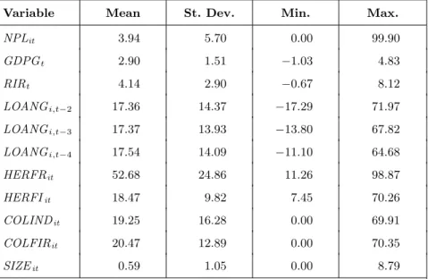
All the information from each individual bank comes from the CCR. Table 1 contains the descriptive statistics of the variables. The period analyzed covers two credit cycles of the Spanish bank-ing sector (from 1984 to 2002), with an aggregate maximum for
Table 1. Descriptive Statistics
Variable Mean St. Dev. Min. Max.
NPLit 3.94 5.70 0.00 99.90 GDPGt 2.90 1.51 −1.03 4.83 RIRt 4.14 2.90 −0.67 8.12 LOANGi,t−2 17.36 14.37 −17.29 71.97 LOANGi,t−3 17.37 13.93 −13.80 67.82 LOANGi,t−4 17.54 14.09 −11.10 64.68 HERFRit 52.68 24.86 11.26 98.87 HERFIit 18.47 9.82 7.45 70.26 COLINDit 19.25 16.28 0.00 69.91 COLFIRit 20.47 12.89 0.00 70.35 SIZEit 0.59 1.05 0.00 8.79
Note:NPLit is the nonperforming loan ratio—that is, the quotient between
nonperforming loans and total loans.GDPGtis the real rate of growth of gross
domestic product.RIRt is the real interest rate, calculated as the interbank
interest rate less the inflation of the period.LOANGitis the rate of the growth
of loans for bank i. HERFRit is the Herfindahl index of bank iin terms of
the amount lent to each region.HERFIit is the Herfindahl index of bankiin
terms of the amount lent to each industry.COLINDitis the percentage of fully
collateralized loans to households over total loans for banki.COLFIRitis the
percentage of fully collateralized loans to firms over total loans for banki.
SIZEit is the market share of bank i. All variables are shown in percentage
points.idenotes the bank andtdenotes the year.
and savings banks, which represent more than 95 percent of total assets among credit institutions (only small credit cooperatives and specialized financial firms are left aside). Some outliers have been eliminated in order to avoid the possibility that a small number of observations, with a very low relative weight over the total sample, could bias the results. Thus, we have eliminated those extreme loan growth rates (i.e., banks with a loan growth rate lower or higher than the 5th and 95th percentile, respectively).
Results appear in the first column of table 2 (labeled “Model 1”). As expected, since we take first differences of equation (1) and
T able 2. GMM Estimation Results of Equation (1) Using DPD (Arellano and Bond 1991) Mo del 1 Mo del 2 Mo del 3 Mo del 4 V ariables Co efficien t S E Co efficien t S E Co efficien t S E Co efficien t S E NPL i,t − 1 0 . 5524 0 . 0887*** 0 . 5520 0 . 0889*** 0 . 5499 0 . 0841*** 0 . 5447 0 . 0833*** M a c roec onomic Char acteristics GDPD t − 0 . 0631 0 . 0135*** − 0 . 0654 0 . 0137*** − 0 . 0709 0 . 0131*** − 0 . 0716 0 . 0134*** GDPG t − 1 − 0 . 0771 0 . 0217*** − 0 . 0770 0 . 0220*** − 0 . 0750 0 . 0212*** − 0 . 0777 0 . 0209*** RIR t 0 . 0710 0 . 0194*** 0 . 0703 0 . 0193*** 0 . 0704 0 . 0195*** 0 . 0711 0 . 0192*** RIR t − 1 0 . 0295 0 . 0103*** 0 . 0292 0 . 0103*** 0 . 0262 0 . 0098*** 0 . 0263 0 . 0101*** Bank Char acteristics LO ANG i,t − 2 − 0 . 0008 0 . 0013 − 0 . 0008 0 . 0013 LO ANG i,t − 3 0 . 0018 0 . 0012 0 . 0018 0 . 0012 LO ANG i,t − 4 ( α ) 0 . 0034 0 . 0012*** 0 . 0029 0 . 0012** | LO ANG i,t − 2 − A VERA GE LO ANG i | 0 . 0004 0 . 0017 | LO ANG i,t − 3 − A VERA GE LO ANG i | − 0 . 0005 0 . 0016 | LO ANG i,t − 4 − A VERA GE LO ANG i | ( β ) 0 . 0025 0 . 0019 LO ANG i,t − 2 − A VERA GE LO ANG t 0 . 0007 0 . 0012 0 . 0011 0 . 0013 LO ANG i,t − 3 − A VERA GE LO ANG t 0 . 0015 0 . 0013 0 . 0014 0 . 0014 LO ANG i,t − 4 − A VERA GE LO ANG t ( α ) 0 . 0025 0 . 0013** 0 . 0020 0 . 0013 ( continue d )
T able 2 (con tin ued). GMM Estimation Results of Equation (1) Using DPD (Arellano and Bond 1991) Mo del 1 Mo del 2 Mo del 3 Mo del 4 V ariables Co efficien t S E Co efficien t S E Co efficien t S E Co efficien t S E Bank Char acteristics (c ontinue d) | LO ANG i,t − 2 − A VERA GE LO ANG t | − 0 . 0026 0 . 0018 | LO ANG i,t − 3 − A VERA GE LO ANG t | 0 . 0017 0 . 0017 | LO ANG i,t − 4 − A VERA GE LO ANG t | ( β ) 0 . 0029 0 . 0018 HERFR it 0 . 0212 0 . 0096** 0 . 0209 0 . 0097** 0 . 0207 0 . 0098** 0 . 0218 0 . 0099** HERFI it − 0 . 0032 0 . 0094 − 0 . 0025 0 . 0095 − 0 . 0038 0 . 0098 − 0 . 0026 0 . 0097 COLFIR it 0 . 0034 0 . 0063 0 . 0034 0 . 0063 0 . 0034 0 . 0065 0 . 0046 0 . 0065 COLIND it − 0 . 0125 0 . 0072* − 0 . 0125 0 . 0072* − 0 . 0141 0 . 0073* − 0 . 0141 0 . 0074* SIZE it 0 . 0199 0 . 0482 0 . 0153 0 . 0486 0 . 0213 0 . 0475 0 . 0261 0 . 0484 Time Dummies No No No No No. Observ ations 868 868 868 868 Time P erio d 1984–2002 1984–2002 1984–2002 1984–2002 Sargan T est [ χ (2) 138 ]/p-v alue 124 . 76 0 . 78 125 . 56 0 . 77 123 . 85 0 . 80 122 . 86 0 . 82 First-Order Auto correlation (m 1 ) − 5 . 43 − 5 . 37 − 5 . 36 − 5 . 28 Second-Order Auto correlation (m 2 ) − 1 . 27 − 1 . 4 − 1 . 34 − 1 . 24 T est Asymmetric Impact (p-v alue) α + β =0 — 0 . 01 — 0 . 01 α − β =0 — 0 . 84 — 0 . 73 Note: See note in table 1 for a description of the v ariables. NPL it , HERFR it , HERFI it , COLFIR it , and COLIND it are treated as endogenous using three lags for NPL it and tw o for the others. Robust SE rep orted. *, **, and *** are significan t a t the 10 p ercen t, 5 p ercen t, and 1 p ercen t lev els, resp ectiv ely .
not second order. A Sargan test of validity of instruments is also fully satisfactory. The results of the estimation are robust to heteroskedasticity.
Regarding the explanatory variables, there is persistence in the
NPLvariable. The macroeconomic control variables are both
signif-icant and have the expected signs. Thus, the acceleration of GDP, as well as a decline in real interest rates, brings about a decline in problem loans. The impact of interest rates is much more rapid than that of economic activity. The more concentrated the credit port-folio in a region, the higher the problem loan ratio, while industry concentration is not significant. Collateralized loans to households are less risky (10 percent level of significance), mainly because these are mortgages that, in Spain, have the lowest credit risk. The para-meter of the collateralized loans to firms, although positive, is not significant. The size of the bank does not have a significant impact on the problem loan ratio.
Finally, regarding the variables that are the focus of our paper, the rate of loan growth lagged four years is positive and significant (at the 1 percent level). The loan growth rate lagged three years is also positive, although not significant. Therefore, rapid credit growth today results in lower credit standards that, eventually, bring about higher problem loans.
The economic impact of the explanatory variables is significant. The long-run elasticity of GDP growth rate, evaluated at the mean
of the variables, is−1.19; that is, an increase of 1 percentage point in
the rate of GDP growth (i.e., GDP grows at 3 percent instead of at
2 percent) decreases the NPLratio by 30.1 percent (i.e., it declines
from 3.94 percent to 2.75 percent). For interest rates, a
100-basis-point increase brings about a rise in theNPLratio of 21.6 percent.
Regarding loan growth rates, an acceleration of 1 percent in the growth rate has a long-term impact of a 0.7 percent higher problem loan ratio.
We have performed numerous robustness tests. Model 2 (the second column of table 2) tests for the asymmetric impact of loan expansions and contractions. We augment model 1 with the absolute
value of the difference between the loan credit growth of banki in
yeartand its average over time. All model 1 results hold, but it can
be seen that there is some asymmetry: rapid credit growth of a bank (i.e., above its own average loan growth) increases nonperforming
loans, while slow growth (i.e., below average) has no significant
impact on problem loans.12 If instead of focusing on credit growth
of bank i(either alone or compared to its average growth rate over
time), we look at the relative position of bankiin respect to the rest
of the banks at a point in time (i.e., at each yeart), we find that the
relative loan growth rate lagged four years still has a positive and
significant impact on bank i’sNPL ratio (model 3, third column of
table 2). The parameter of relative credit growth lagged three years is positive but not significant. The rest of the variables keep their sign and significance. Model 4 (the last column of table 2) shows that there is asymmetry in the response of nonperforming loans to credit growth. When banks expand their loan portfolios at a speed above the average of the banking sector, future nonperforming loans increase, while there is no significant effect if the loan growth is below
the average.13 Finally, the former results are robust to changes in
the macroeconomic control variables (not shown). If we substitute time dummies for the change in the GDP growth rate and for the real interest rate, the loan growth rate is still positive and signifi-cant in lag 4 (although at the 10 percent level) and, again, positive (although not significant) in lag 3.
All in all, we find a robust statistical relationship between rapid credit growth at each bank portfolio and problem loans later on. The lag is around four years, so bank managers and short-term investors (including shareholders) might have incentives to foster credit growth today in order to reap short-term benefits to the expense of long-term bank stakeholders, including depositors, the deposit guarantee fund, and banking supervisors.
2.2 Probability of Default and Credit Growth
Instead of focusing on bank-aggregated-level credit risk measures, in this section we analyze the probability of default at an individual
12
Note that in model 1, regression results are the same for the variable rate of
growth of loans in bankiat yeartas they are for the difference between the
for-mer variable and the average rate of growth of loans of bankialong time. That is
because the latter term is constant over time for each bank and disappears when we take first differences in equation (1).
13Note that the relevant test here is to test ifα+β(andα−β) is significant,
loan level and its relation to the cyclical position of the bank credit policy. The hypothesis is that, for the reasons explained in section 1 above, those loans granted during credit booms are riskier than those granted when the bank is reining in loan growth. That would pro-vide a rigorous empirical microfoundation for prudential regulatory devises aimed at covering the losses embedded in policies regarding rapid credit growth.
In order to test the former hypothesis, we use individual loan data from the CCR. We focus on new loans granted to nonfinancial firms with a maturity larger than one year and keep track of them the following years. We study only financial loans (i.e., excluding receivables, leasing, etc.), which are 60 percent of the total loans to nonfinancial firms in the CCR, granted by commercial and savings banks. The equation estimated is
Pr(DEFAULTijt+k= 1) =F(θ+α(LOANGit−averageLOANGi)
+βLOANGit−averageLOANGiχLOANCHARiit
+δ1DREGi+δ2DINDi+δ3BANKCHARit+ϕt+ηi), (2)
where we model the probability of default of loanj, in bank i, some
kyears after being granted (i.e., att+ 2,t+ 3, andt+ 4)14as a
logis-tic function [F(x) = 1/(1 +exp(−x))] of the characteristics of that
loan (LOANCHAR), such as its size, maturity (i.e., between one
and three years and more than three years), and collateral (fully collateralized or no collateral); a set of control variables (i.e., the
region where the firm operates, DREG, and the industry to which
the borrower pertains, DIND); and the characteristics of the bank
that grants the loan (BANKCHAR), such as its size and type (i.e.,
commercial or savings bank). We also control for macroeconomic
characteristics, including time dummies (ϕt).
We do not consider default immediately after the loan is granted
(i.e., in t+ 1) because it takes time for a bad borrower to reveal as
14
We consider that a loan is in default when its doubtful part is larger than the 5 percent of its total amount. Thus, we exclude from default small arrears, mainly technical, that are sorted out by borrowers in a few days and that, usually, never reach the following month. The level and the evolution of the probability of default (PD) across time and firm size in Spain can be seen in Saurina and Trucharte (2004). On average, large firms (i.e., those with annual sales above
e50 million) have a PD between four and five times lower than that of small and
such. When granted a loan, a borrower takes the money from the bank and invests it into the project. As the project develops, the borrower is either able to repay the loan and the due interest pay-ments or is not able to pay and defaults. Therefore, it takes time for the default to occur.
Once we have controlled for loan, bank, and time
characteris-tics, we add the relative loan growth rate of bank i at time t with
respect to financial loans granted to nonfinancial firms (LOANGit−
averageLOANGi)—that is, the current lending position of each bank
in comparison to its average loan growth. If α is positive and
sig-nificant, we interpret this as a signal of more credit risk in boom periods when, probably, credit standards are low. On the contrary, when credit growth slows, banks become much more careful in scru-tinizing loan applications; as a result, next-year defaults decrease sig-nificantly. To our knowledge, this is the first time that such a direct test has been run. Additionally, we test for asymmetries in that rela-tionship, as in the previous section. We have considered only those banks with a loan growth rate within the 5th and 95th percentile, to eliminate outliers.
It is very important to control for the great heterogeneity due to firm effects, even more because our database does not contain firm-related variables (i.e., balance sheet and profit and loss variables). For this reason, we have controlled for firm (loan) characteristics using a random effects model, which allows us to take into account the unobserved heterogeneity (without limiting the sample as the conditional model does) assuming a zero correlation between the
firm effects and the rest of the characteristics of the firm.15
Table 3 shows the estimation results for the pool of all loans granted. We observe that the faster the growth rate of the bank, the higher the likelihood to default in the following years. We observe
that α is positive and significant when we consider defaults three
and four years later, and αis positive, although not significant, for
defaults two years after the loan was granted (table 3, columns 1, 3, and 5). As mentioned before, although not reported in table 3, we control for macroeconomic characteristics, region and industry
15We have also estimated a logit model with fixed effects, and the results are
Table 3. GMM Estimation Results of Equation (2) Using a Random Effect Logit Model (Results for Pool of All
Loans Granted)
(1) (2)
Variables Coeff. SE Coeff. SE
Dependent Variable DEFAULTijt+2(0/1) DEFAULTijt+2(0/1)
Bank Characteristics
LOANGit−AVERAGE
LOANGi(α) 0.001 0.001 −0.001 0.001*
|LOANGit−AVERAGE
LOANGi(β) — — 0.005 0.001***
Province Dummies Yes Yes
Industry Dummies Yes Yes
No. Observations 1,823,656 1,823,656
Time Period 1985–2004 1985–2004
Wald Test [χ(2)]/p-value 8,959 0.00 9,121 0.00
Test Asymmetric Impact (p-value)
α+β= 0 — 0.00
α−β= 0 — 0.00
(3) (4)
Variables Coeff. SE Coeff. SE
Dependent Variable DEFAULTijt+3(0/1) DEFAULTijt+3(0/1)
Bank Characteristics
LOANGit−AVERAGE
LOANGi(α) 0.002 0.001*** 0.001 0.001
|LOANGit−AVERAGE
LOANGi|(β) — — 0.001 0.001
Province Dummies Yes Yes
Industry Dummies Yes Yes
No. Observations 1,643,708 1,643,708
Time Period 1985–2004 1985–2004
Wald Test [χ(2)]/p-value 4,800 0.00 4,874 0.00
Test Asymmetric Impact (p-value)
α+β= 0 — 0.00
α−β= 0 — 0.93
Table 3 (continued). GMM Estimation Results of Equation (2) Using a Random Effect Logit Model
(Results for Pool of All Loans Granted)
(5) (6)
Variables Coeff. SE Coeff. SE
Dependent Variable DEFAULTijt+4(0/1) DEFAULTijt+4(0/1)
Bank Characteristics
LOANGit−AVERAGE 0.002 0.001** 0.002 0.002
LOANGi(α)
|LOANGit−AVERAGE — — 0.000 0.002
LOANGi|(β)
Province Dummies Yes Yes
Industry Dummies Yes Yes
No. Observations 1,433,074 1,433,074
Time Period 1985–2004 1985–2004
Wald Test [χ(2)]/p-value 2,992 0.00 3,054
Test Asymmetric Impact (p-value)
α+β= 0 — 0.04
α−β= 0 — 0.55
Note:DEFAULT is a dummy variable that takes 1 if the loan is doubtful and 0
other-wise.LOANGit is the growth rate of all financial credits granted to firms for banki. We
also control for bank size and type (i.e., commercial or savings) and for loan characteristics (i.e., size, maturity, and collateral). Region, industry, and time dummies have been included. *, **, and *** are significant at the 10 percent, 5 percent, and 1 percent levels, respectively.
of the borrowing firm, size and type of the bank lender, and, finally, for size, maturity, and collateral of the loan granted.
We have also investigated if there is an asymmetric impact of loan growth over defaults (columns 2, 4, and 6 in table 3). In good times, when loan growth of each bank is above its average, we find a positive and significant impact on future defaults (two, three, and four years later). However, in bad times, with loan growth below the bank’s average, there is no impact on defaults. Thus, this asymmet-ric effect reinforces the conclusions about too-lax lending policies during booms.
To test the robustness of the former results, table 4 shows the estimation of the model when the loan growth rate of the bank is introduced without any comparison to its average value. The results obtained are exactly the same: there is no effect on the probability of
T able 4. GMM Estimation Results of Equation (2) Using a Random Effect Logit Mo del (Loan Gro wth Rate of Bank In tro duced without Comparison to Its Av erage V alue) V ariables Co eff. SE Co eff. SE Co eff. SE Dep endent V ariable DEF A U L Tijt +2 (0/1) DEF A U L T ijt +3 (0/1) DEF A U L T ijt +4 (0/1) Bank Char acteristics LO ANG it 0.001 0.001 0.002 0.001*** 0.002 0.001*** Pro vince Dummies Ye s Ye s Ye s Industry Dummies Ye s Ye s Ye s No. Observ ations 1,823,656 1,643,708 1,433,074 Time P erio d 1985–2004 1985–2004 1985–2004 W ald T est [ χ (2)]/p-v alue 8,966 0.00 4,802 0.00 2,987 0.00 Note: DEF A U L T is a dumm y v ariable that tak es 1 if the loan is doubtful and 0 otherwise. LO ANG it is the gro wth rate of all financial credits gran ted to firms for bank i. W e also con trol for bank size and ty p e (i.e., commercial or sa vings) and for loan characteristics (i.e., size, maturit y , and collateral). Region, industry , and time dummies ha v e b een included. *, ** and *** are significan t a t the 10 p ercen t, 5 p ercen t, and 1 p ercen t lev els, resp ectiv ely .
default int+ 2 and a positive and significant one on the likelihood of
default in t+ 3 andt+ 4.
In terms of the economic impact, the semi-elasticity of the credit
growth is 0.13 percent for default in t+ 3 (0.13 percent in t+ 4),16
which means that if a bank grows 1 percentage point, then the
like-lihood of default int+ 3 is increased by 0.13 percent (0.13 percent
int+ 4). If a bank was expanding its loan portfolio at one standard
deviation above the average rate of growth, the impact would be 1.9 percent (1.9 percent). Thus, the economic impact estimated is low for the period analyzed and the sample considered, despite the significance of the variables.
All in all, the previous results show that in good times, when credit is growing rapidly, credit risk in bank loan portfolios is also increasing.
2.3 Collateral and Credit Growth
This section provides evidence of the behavior of banks in terms of their credit policies along the business cycle. The argument so far has been that too-rapid credit growth comes with lower credit stan-dards and, later on, manifests in a higher number of problem loans. Here, we provide some complementary evidence based on the tight relationship between credit cycles and business cycles. We argue that banks adjust their credit policies depending on the business-cycle position. For instance, in good times, banks relax credit stan-dards and are prepared to be more lenient in collateral requirements. On the other hand, when a recession arrives, banks toughen credit conditions and, in particular, collateral requirements.
If the hypothesis presented in the former paragraph is true, we would have complementary evidence to support prudential regula-tory policies. If it is true that, during boom times, loan portfolios are increasingly loaded with higher expected defaults, then it should also be true that other protective devises for banks, such as collateral, are
eroded.17 The following equation allows us to test the relationship
between collateral and economic cycle.
16The marginal effect of thek-variable is computed asME
k= d[Probdx(y=1|x¯)]
k =
Λ( ˆβ¯x)[1−Λ( ˆβx¯)] ˆβk. Then, the semi-elasticity is given byMEk/Average Default.
17It might also be the case that, during good times, banks decrease credit risk
Pr(Collateralijklt = 1) =F(θ+αGDPGt−1
+β|GDPGt−1−Average GDP|+Control Variablesijklt) (3) A full description of model 3 and its control variables is in
Jim´enez, Salas, and Saurina (forthcoming). Here we only focus
on the impact of GDP growth on collateral, controlling for the other determinants of collateral. The variable on the left-hand side takes the value of 1 if the loan is collateralized and 0 otherwise.
j refers to the loan, i refers to the bank, k refers to the market,
lrefers to the firm (borrower), andtrefers to the time period (year).
We estimate equation (3) using a probit model. As control vari-ables, we use borrower characteristics (i.e., if they were in default the year before or the year after the loan was granted, their indebt-edness level, and their age as a borrower), bank characteristics (size, type of bank, and its specialization in lending to firms), character-istics of the borrower-lender relationship (duration and scope), and other control variables (such as the level of competition in the loan market, the size of the loan, and the industry and region of the
borrower).18
The database used is the CCR. We focus on all new financial
loans abovee6,000 with a maturity of one year or more, granted by
any Spanish commercial or savings bank to nonfinancial firms every year during the time period between December 1984 and December 2002. We exclude commercial loans, leasing, factoring operations, and off-balance-sheet commitments for homogeneity reasons.
The first column in table 5 shows the results of estimating model 3 for the pool of loans, nearly two million loans. There is a negative and significant relationship between GDP growth rates and collateral; that is, in good times banks lower collateral require-ments, and they increase them in bad times. In terms of the impact,
the semi-elasticity ofGDPG is −3.1 percent, which means that an
competition among banks. The opposite would happen in bad times, when bank managers would tighten credit spreads. Unfortunately, our database does not allow us to test this hypothesis.
18Jim´enez, Salas, and Saurina (forthcoming) contains a similar analysis on a
different sample of loans and using a different estimation procedure (i.e., fixed effects).
T able 5. GMM Results of Equation (3) Using a Probit Mo del All Borro w ers (1) (2) All T erms All T erms V ariables Co eff. SE Co eff. SE Dep endent V ariable COLLA TERAL t (1 / 0) M a c roec onomic Char acteristics GDPG t − 1 ( α ) − 0.045 0.001*** − 0.047 0.001*** | GDPG t − 1 − A ver age GDPG t − 1 | ( β ) —— − 0.011 0.002*** Regional Dummies Ye s Ye s Industry Dummies Ye s Ye s No. Observ ations 1,972,336 1,972,336 Time P erio d 1985–2002 1985–2002 χ 2 Co v ariates / p-v alue 279,056 0.00 279,007 0.00 T est Asymmetric Impact (p-v alue) α + β =0 — 0.00 α − β =0 — 0.00 ( continue d )
T able 5 (con tin ued). GMM Estimation Results of Equation (3) Using a Probit Mo del Old Borro w ers New Borro w ers (3) (4) (5) (6) Long T erm Short T erm Long T erm Short T erm V ariables Co eff. SE Co eff. SE Co eff. SE Co eff. SE Dep endent V ariable COLLA TERAL t (1 / 0) M a c roec onomic Char acteristics GDPG t − 1 ( α ) − 0.067 0.001*** − 0.021 0.002*** − 0.054 0.002*** − 0.019 0.004*** | GDPG t − 1 − A ver age GDPG t − 1 | ( β ) − 0.004 0.002** − 0.026 0.004*** 0.002 0.004 − 0.027 0.007*** Regional Dummies Ye s Ye s Ye s Ye s Industry Dummies Ye s Ye s Ye s Ye s No. Observ ations 823,340 723,924 254,755 170,317 Time P erio d 1985–2002 1985–2002 1985–2002 1985–2002 χ 2 Co v ariates / p-v alue 147,630 0.00 39,368 0.00 41,708 0.00 13,668 0.00 T est Asymmetric Impact (p-v alue) α + β =0 0.00 0.00 0.00 0.00 α − β =0 0.00 0.14 0.00 0.26 Note: COLLA TERAL is a dumm y v ariable that tak es 1 if the loan gran ted to a firm is collateralized and 0 otherwise. GDPG is the real gro wth rate of gross domestic pro duct. W e also con trol for bank size, ty p e (i.e., commercial, sa vings, or co op erativ e), and lending sp ecialization; for b orro w e r characteristics (i.e., if they w ere in default the y ear b efore or the y ear after the loan w a s gran ted, their indebtedness lev el, and their age as a b orro w er); for characteristics of the b orro w er-lender relationship (duration and scop e); and for the lev el of comp etition in the loan mark et, the size of the loan, and the industry and region of the b orro w er. ** and *** are significan t at the 5 p ercen t and 1 p ercen t lev els, resp ectiv ely .
increase of 1 percentage point inGDPGreduces the likelihood of col-lateral by 3.1 percent. In the bond market, Altman, Resti, and Sironi (2002) find evidence of a positive and significant correlation between the probability of default (PD) and the loss given default (LGD). Focusing on the loan market, our results show that the positive cor-relation between PD and LGD need not hold since—as the recession approaches (and the PD increases)—banks take more collateral on
their loans, which might decrease the LGD.19
The cyclical behavior of banks regarding collateral is not sym-metric. Column 2 in table 5 shows that the likelihood to pledge collateral decreases proportionally more in upturns than it increases in downturns, as the negative and significant value of the parameter of the absolute value of the difference between GDP rate of growth
and its average across the period studied points out (i.e.,−0.092 in
upturns versus −0.058 in downturns). Despite the asymmetry, the
negative relationship between loan PD and LGD still might hold. Moreover, from a prudential point of view, there are even more concerns regarding the too-lax credit policies maintained by banks during upturns.
Credit markets are segmented across borrowers and across matu-rities. Therefore, it might be possible that the former aggregated results do not hold for particular market segments. To carry out this robustness exercise, the database is split into two groups: short term (maturing at one to three years) and long term (maturing at more than three years). A second classification of the loans relates to the experience of the borrower. One group of loans, labeled “old,” contains those loans from borrowers about whom, at the time the loan is granted, there is already past information in the database (for instance, if they were in default the previous year). The other group of loans, which we call “new,” is from borrowers obtaining a loan for the first time. Table 5 (columns 3–6) shows that, although there are some differences across the maturity of borrowers and across old and new borrowers, the main results hold. For old borrowers, the impact of the business cycle on collateral policy is larger for long-term loans than for short-long-term ones. We find the same result across new borrowers, but the magnitude of the decline in collateral as the
economy improves is lower. For short-term loans—both old and new borrowers—collateral requirements decline during upturns but do not increase during downturns, either because the firm has no col-lateral to pledge or because banks put in place other strategies to recover their short-term loans.
3. A New Prudential Tool
The former section has shown clear evidence of a relationship between rapid credit growth and a deterioration in credit standards that eventually leads to a significant increase in credit losses. Bank-ing regulators, aware of this behavior and concerned about long-term solvency of individual banks as well as the stability of the whole banking system, might wish to implement some devices in order to alleviate the market imperfection.
Borio, Furfine, and Lowe (2001) contains a detailed discussion of procyclicality and banking regulator responses. There has been a lot of discussion about the impact of capital requirements on the cyclical
behavior of banks.20 Here, we want to focus on loan loss provisions
since we think that they are the proper instrument to deal with expected losses. Thus, we propose a new prudential provision that addresses the fact that credit risk builds up during credit boom peri-ods. This new provision is in addition to the already existing specific and general provisions. The general provision can be interpreted as a provision for the inherent or latent risk in the portfolio—that is, an average provision across the cycle. The new loan loss provision (or the third component of the total loan loss provision) is based on the credit-cycle position of the bank in such a way that the higher the credit growth of the individual bank, the more it has to provision. On the contrary, the lower the credit growth, the more provisions the bank can liberate from the previously built reserve. Analytically, we can write
LLPtotal=specif.+g∆C+α(∆C−γCt−1), (4)
20The issue of procyclicality of capital requirements has drawn a lot of
atten-tion (Dan´ıelsson et al. 2001, Kashyap and Stein 2004, and Gordy and Howells 2004, to name a few).
where the total loan loss provision (LLPtotal) has three components:
(i) the specific provision (specif.), (ii) the latent provision (applied
on each new loan granted to cover the average credit risk, g), and
(iii) the countercyclical, or forward-looking, provision, where Ct−1
is the stock of loans for the previous period, γ is the average loan
growth rate across banks and across a lending cycle, and ∆C is the
absolute growth in total loans. Thus, when the loan portfolio grows above the average historical growth rate, the provision is positive, and it is negative otherwise.
Note that the provision is positive in boom periods and nega-tive during recessions. The more distant the bank behavior is from the total system, the larger the provisioning impact. The underlying idea is quite simple: the more rapid the credit growth, the higher the increase in market share and, presumably, following our empirical results, the higher the credit risk assumed by the bank and, there-fore, the higher the provision. The asymmetry found in some of the results of the former section (see table 2) points toward an increase in loan loss provisions in good times, when credit risk increases and there is rapid credit growth, and allowing the previously built loan loss reserves to be depleted in downturns, when the former rapid credit growth materializes as loan losses.
Our proposal is a very simple and intuitive prudential tool to cope with credit risk linked to cyclical lending policies. The provi-sion is not expected to replace the existing proviprovi-sions but rather to reinforce them. Therefore, we would have specific provisions for impaired assets already individually identified, plus provisions to cover inherent losses in homogeneous groups of loans (i.e., losses incurred but not yet identified in individual loans), as well as pro-visions that take into account the position of the bank in the credit cycle and, thus, its credit risk profile.
The third component of LLPtotal, the countercyclical one, has
been considered in our proposal as an additional loan loss provi-sion. Alternatively, it could be included in capital requirements (for
instance, asked through pillar 2 of the Basel II framework).21
Bank-ing supervisors, accordBank-ing to their experiences regardBank-ing lendBank-ing cycles and credit risk, might ask banks to hold higher capital levels
during booms in order to take into account future problem loan developments. Note that this proposal might contribute to allevi-ate potential concerns, if any, about increased capital procyclicality within the Basel II framework.
3.1 Simulations
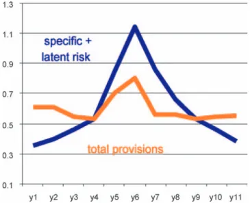
One way to understand the workings of the provision put forward is through a simulation exercise. We simulate a full economic and lending cycle in eleven years. During the first two years, the econ-omy is expanding at full steam, which means rapid credit growth and very low specific loan loss provisions (as a result of low problem loan ratios). From year 3 onward credit growth decreases and prob-lem loans increase with a subsequent increase in specific provisioning requirements. In year 6 the trough is reached with a maximum in provisioning requirements and a minimum in lending growth. From year 7 onward the credit and the economy recover and specific pro-visions decline. Figure 1 shows the evolution of loan loss propro-visions over total loans during the eleven years. The evolution of the spe-cific provision plus the general (latent risk) provision (i.e., the first two parts of our provisioning formula (4)) is quite cyclical, with a significant rise around the trough period.
Regarding the third component of the total loan loss provision, when loan growth rates are above the average loan growth rate (i.e., the first three years in our simulation), its amount is posi-tive, charged in the profit and loss account (P&L), and accrued in a provision fund or reserve account. When loan growth starts to dip below the average (between years 4 and 9), the amount is negative
and is accrued in the P&L from the previously built fund.22 From
year 10 onward the provision resumes a positive value (as a result of a new expansionary credit cycle), and the fund is being built up again.
What is the final impact of the new provision over a frame-work that already has a specific and a general provision? The total loan loss provision is smoother than the sum of the specific and
22Of course, it is understood that the fund cannot be negative; that is, the
bank is not allowed to write as income in the P&L something that has not been previously built up.
Figure 1. Simulation Exercise: Loan Loss Provisions as a Percentage of Total Loans
general provisions (figure 1). But the smoothing is far from total. There is still quite a significant variation of total loan loss provi-sions across the credit cycle. Of course, during recesprovi-sions proviprovi-sions reach the maximum amount, as the specific one dominates the land-scape. However, in true boom periods (i.e., years 1 and 2) when loan growth is extremely high, provisioning requirements through the third component of the provision are significant. The new pro-vision is countercyclical, but it does not have a significant impact on total loan loss provisions unless the variability in credit growth rates is extreme, which—for most of the banks—is not the case. At the same time, the volatility of profits is somewhat lower through the cycle.
4. Policy Discussion
The empirical results of the former section provide a rationale for countercyclical loan loss provisions, apart from those covering impaired assets or the latent risk in the loan portfolio. However, accounting frameworks do not fully recognize such a coverage. For
instance, although from a prudential point of view there is a rationale for setting aside provisions since the loan is granted, accountants are
reluctant to allow it.23
Since January 2005, all European Union firms (either banks or nonfinancial firms) with quoted securities in any EU organized mar-ket have to comply with International Financial Reporting Stan-dards (IFRS, formerly called International Accounting StanStan-dards, or IAS). That means a change in the provisioning system based on specific and general provisions. From 2005 onward, banks have to set aside provisions to cover individually identified impaired assets; for homogeneous loan portfolios, they will be required to cover losses incurred but not yet identified in individual loans. IAS 39 does not allow banks to set aside provisions for future losses when a loan is granted. Therefore, the new standards do not perfectly match the prudential concerns of banking regulators. Borio and Tsatsaronis (2004) show a way to sort out this problem through a decoupling of objectives (i.e., one is to provide unbiased information; the other is to instill a degree of prudence). We believe a more fundamental ques-tion is, what purpose should the accounting framework serve and, more importantly, at what price? Financial stability concerns and, therefore, prudent accounting should probably be higher on the list of priorities, especially since there is overwhelming evidence of earn-ings management. The incentives to alter the accounting numbers
will not disappear with IAS.24 If investors might not, in any case,
get the unbiased figures, there might be room for instilling prudent behavior through the accounting rules.
Alternatively, if accounting principles are written in a way that does not allow for sheltering prudential concerns, banking regula-tors might try other devices in order to counterbalance the nega-tive impact of excessive decreases in credit standards during boom periods. For instance, pillar 2 of the new capital framework put for-ward by supervisors in Basel II might include a stress test of capital requirements that might be based along the lines developed here for
23
That is not the case with insurance companies, where the technical provision to cover the risk incurred appears just after the insurance policy has been sold to the customer.
24For a theoretical rationale of income smoothing, see (among others)
the new provision. In a sense, if the accounting framework does not provide enough flexibility to banking supervisors, they should find it through the allowed supervisory discretion of pillar 2.
Either as an additional provision or as a capital requirement, the third component of total loan loss provisions will help to counter the cyclical behavior of own funds in Basel II. Basel I was not properly tracking banks’ risks. Basel II is meant to tie capital requirements more closely to risk. Capital requirements will increase during reces-sions as the probability of default increases. However, the evidence provided in this paper argues that (ex ante) credit risk increases during boom periods. Therefore, without interfering with Basel II pillar 1 capital requirements, pillar 2 adjustment might help to take into account those increases in ex ante credit risk and, somehow,
soften the procyclicality of capital requirements.25
Rajan (1994) discusses possible regulatory interventions that would reduce the expansionary bias in lending policies—among them, decreasing the amount of loanable funds or imposing credit controls. However, both proposals do not seem very feasible since they might have other negative, unintended consequences, as the author recognizes. Alternatively, close monitoring of bank portfo-lios by supervisors, and the corresponding penalties, might be the answer. However, that will increase the cost of supervision substan-tially. Our loan loss provision proposal is inexpensively monitored and easily available for bank supervisors. Moreover, it is not designed to curtail credit growth but to account for the negative impact of too-lax lending policies. It is up to each bank manager to decide its lending policy, but if the lending policy is reckless, loan loss provi-sions should be proportionally higher to account for future higher credit losses.
This paper also has some implications in terms of financial infor-mation disclosure and transparency. It is argued that more disclosure of information by banks will help investors to discipline bank man-agers and, therefore, to help banking supervisors as well. In fact, that is the main rationale for pillar 3 of Basel II. However, some recent research (Morris and Shin 2002) points toward a more-nuanced posi-tion regarding the welfare achievements of more transparency and
25The loan loss provision we propose here might work as the “second
disclosure and the above-mentioned widespread existence of earnings management. In fact, Rajan (1994) finds what he calls a counterin-tuitive comparative statics: “Allowing banks to fudge their account-ing numbers and to maintain secret (sic) reserves can improve the quality of their lending decisions.”
The new provision is fully transparent. Investors and, more gen-erally, any bank stakeholder could “undo” its effects since they only need to look at the lending growth rate of the bank and the average of the system. Of course, transparency could improve even more if regulators make it compulsory to release the amount of the stress provision in the annual report of each bank. Here, we are not try-ing to manage earntry-ings or, more precisely, to smooth banks’ income through that provision. Instead, we are just trying to cope with latent risks in bank loan portfolios in a way that is fully transparent and not properly addressed by IAS or even Basel II capital require-ments. In fact, it might be possible that our proposal could con-tribute to a decline in income-smoothing practices across banks since (at least partially) some of their causes would be covered by the new provision. Thus, contrary to Rajan, banking regulators would have no need to allow banks more discretion to “fudge” their accounts since the regulatory framework would allow for an appropriate cov-erage of latent risks in good times and a lower impact on the P&L in bad periods that would result in a less volatile pattern for profits through the cycle.
Banco de Espa˜na has applied the so-called statistical provision
from mid-July 2000 onward. It is a countercyclical provision. When the three currently existing loan loss provisions (i.e., specific, gen-eral, and statistical) are added up through an economic cycle, the quotient between total loan loss provisions and total loans remains almost constant along time. Accountants did not ever like this total smoothing effect along the credit cycle. The new provision that we have developed in this paper does not have those drawbacks. First of all, the quotient between total loan loss provisions and total loans shows a cyclical pattern (i.e., increases in bad times), but that pattern is much less pronounced than before (figure 1). From a prudential point of view, it is very important that total loan loss provisions are relatively high in the peak of the lending boom. Secondly, although total loan loss provisions are high in boom peri-ods, the maximum is reached around the recession, when impaired
assets are also at their maximum. Thus, loan loss provisions are not completely smooth along the business cycle.
5. Conclusions
Increasing banking competition—coupled with agency problems, strong balance sheets, and some other characteristics of banking markets (such as risk-related capital requirements, imperfections in the equity market, and maturity mismatches)—may bring about lower credit standards that translate into too-expansionary credit policies and, eventually, higher loan losses. Therefore, a bank regu-lator concerned about the negative effects of too-rapid credit growth on individual banks’ solvency and on the whole stability of the bank-ing system might use some prudential tools in order to curtail exces-sive lending during boom periods and, by the same token (although in the opposite direction), too-conservative credit policies during recessions.
The empirical literature on the relationship between excessive loan growth and credit risk is scant. The first contribution of this paper is to provide more precise and robust evidence of a positive, although quite lagged, relationship between rapid credit growth and future nonperforming loans of banks. Moreover, we also find a direct relation between the phase of the lending cycle and the quality and standards of the loans granted. During lending booms, riskier bor-rowers obtain funds, and collateral requirements are significantly decreased. Lower credit standards and a substantial lag between decisions made on loan portfolios and the final appearance of loan losses point toward credit risk significantly increasing during good times. Therefore, credit risk increases in boom periods, although it only pops up as loan losses during bad times.
The second contribution of this paper is to develop a loan loss provision (i.e., a prudential tool) that takes into account the former developments. The idea is that banks should provision during good times for the increasing risk that is entering their portfolios and that will only reveal as such with a lag. On the other hand, in bad times banks could use the reserves accumulated during boom peri-ods in order to cover the loan losses that appear but that entered the portfolio in the past. Thus, we develop a countercyclical provision
that is a direct answer to the robust empirical finding of credit risk increasing in good times.
Accounting frameworks usually do not allow for countercyclical provisioning—that is, for the coverage today of latent credit risk in banks’ portfolios. Therefore, given the interest of supervisors in a prudent coverage of risks, it might be possible to transform the for-mer countercyclical provision into a capital requirement based on a stress test included in pillar 2 of Basel II, the new regulatory capital framework for banks. In doing that, those that have shown concerns about increased procyclicality of Basel II might find some help.
All in all, the paper combines theoretical arguments with robust empirical findings to provide the rationale for a countercyclical loan loss provision. The paper is a contribution to the intense debate among supervisors and academics on the proper tools to enhance financial stability.
References
Akella, S., and S. Greenbaum. 1988. “Savings and Loan
Owner-ship Structure and Expense-Preference.”Journal of Banking and
Finance 12 (3): 419–37.
Altman, E., A. Resti, and A. Sironi. 2002. “The Link Between Default and Recovery Rates: Effects on the Procyclicality of Regulatory Capital Ratios.” BIS Working Paper No. 113. Arellano, M., and S. Bond. 1991. “Some Tests of Specification
for Panel Data: Monte Carlo Evidence and an Application to
Employment Equations.” Review of Economic Studies 58 (2):
277–97.
Asea, P., and B. Blomberg. 1998. “Lending Cycles.” Journal of
Econometrics 83 (1–2): 89–128.
Ayuso, J., D. P´erez, and J. Saurina. 2004. “Are Capital Buffers
Procyclical? Evidence from Spanish Panel Data.” Journal of
Financial Intermediation 13 (2): 249–64.
Basel Committee on Banking Supervision. 2004. “International Convergence of Capital Measurement and Capital Standards: A Revised Framework.” Bank for International Settlements (June).