Learning: PAC-Bayes, Flat Minima,
and Generative Models
Gintare Karolina Dziugaite
Supervisor: Prof. Z. Ghahramani
Department of Engineering
University of Cambridge
This dissertation is submitted for the degree of
Doctor of Philosophy
I hereby declare that except where specific reference is made to the work of others, the contents of this dissertation are original and have not been submitted in whole or in part for consideration for any other degree or qualification in this, or any other university. This dissertation is my own work and contains nothing which is the outcome of work done in collaboration with others, except as specified in the text and Acknowledgements. This dissertation contains fewer than 65,000 words including appendices, bibliography, footnotes, tables and equations and has fewer than 150 figures.
Gintare Karolina Dziugaite December 2018
My first exposure to research was due to Wei Ji Ma, who accepted me for a summer internship in Computational Neuroscience despite the fact that I had only just completed my undergraduate degree in Mathematics and had no prior research experience. Working with Weiji changed my perspective on research as a career choice. I am grateful to Weiji for encouraging me to apply to PhD programs.
I would like to thank my supervisor Zoubin Ghahramani for supporting my decision to transition into machine learning research. Zoubin quickly directed me to interesting projects that resulted in publications, motivating me to continue my research career. I was very fortunate to have an advisor who was an expert in so many different areas of machine learning.
Much of the research reported in this thesis was carried out or initiated while I was a visiting student in the “Foundations of Machine Learning” program at the Simons Institute for the Theory of Computing at UC Berkeley. I would like to explicitly thank Peter Bartlett, Shai Ben-David, Dylan Foster, Matus Telgarsky, and Ruth Urner for helpful discussions. I would also like to thank Bharath Sriperumbudur for technical discussions regarding the work described in Chapter 5.
I am very grateful to my parents who were willing to help at any time and in any way they could, who visited me for months at a time, travelled with me to conferences, and helped care for my children while I was working unreasonable hours.
I am most thankful for my husband’s never-ending support.
Last but not least, I would like to thank the hyper competitive deep learning research community for pushing me to exceed my rest-to-work limits while raising two small children. Under different, more relaxed, conditions, I might have gotten much less work done.
In this work, we construct generalization bounds to understand existing learning algorithms and propose new ones. Generalization bounds relate empirical performance to future expected performance. The tightness of these bounds vary widely, and depends on the complexity of the learning task and the amount of data available, but also on how much information the bounds take into consideration. We are particularly concerned with data and algorithm-dependent bounds that are quantitatively nonvacuous. We begin with an analysis of stochastic gradient descent (SGD) in supervised learning. By formalizing the notion of flat minima using PAC-Bayes generalization bounds, we obtain nonvacuous generalization bounds for stochastic classifiers based on SGD solutions. Despite strong empirical performance in many settings, SGD rapidly overfits in others. By combining nonvacuous generalization bounds and structural risk minimization, we arrive at an algorithm that trades-off accuracy and generalization guarantees. We also study generalization in the context of unsupervised learning. We propose to use a two sample test statistic for training neural network generator models and bound the gap between the population and the empirical estimate of the statistic.
List of figures xv
List of tables xvii
Notation 1
Introduction 3
1 Statistical Learning Theory 9
1.1 Supervised learning . . . 10
1.1.1 Loss functions . . . 11
1.1.2 Empirical risk minimization and PAC-learning . . . 12
1.1.3 Bounding the sample complexity: VC dimension and Rademacher complexity . . . 13
1.1.4 Structural Risk Minimization . . . 15
1.1.5 Minimum Description Length . . . 17
1.2 PAC-Bayes . . . 17
1.2.1 KL divergence and the PAC-Bayes theorem . . . 18
1.2.2 Bounds . . . 19
1.2.3 Optimal Prior and Posterior . . . 19
1.2.4 Gibbs posteriors in (generalized) Bayesian Inference . . . 21
1.2.5 PAC-Bayes risk bound as an optimization objective . . . 23
1.3 Algorithms and Stability . . . 24
1.3.1 Stochastic Gradient Descent . . . 25
1.3.2 Stability of SGD . . . 26
1.4 Differential privacy . . . 26
2 Nonvacuous Generalization Bounds for Deep (Stochastic) Neural Networks 29 2.1 Introduction . . . 29
2.1.1 Understanding SGD . . . 30
2.1.2 Approach . . . 32
2.2 Bounds . . . 34
2.2.1 Inverting KL bounds . . . 34
2.2.2 Learning Algorithm . . . 35
2.3 PAC-Bayes bound optimization . . . 35
2.3.1 The Prior . . . 36
2.3.2 Stochastic Gradient Descent . . . 37
2.3.3 Final PAC-Bayes bound . . . 37
2.4 Approximating KL−1(q|c) . . . 37
2.5 Network symmetries . . . 38
2.5.1 Bounds from mixtures . . . 38
2.6 Experiments . . . 40
2.6.1 Dataset . . . 40
2.6.2 Initial network training by SGD . . . 41
2.6.3 PAC-Bayes bound optimization . . . 41
2.6.4 Reported values . . . 42
2.7 Results . . . 42
2.8 Comparing weights before and after PAC-Bayes optimization . . . 43
2.9 Evaluating Rademacher error bounds . . . 44
2.9.1 Experiment details . . . 46
2.9.2 Results . . . 46
2.10 Related work . . . 47
2.11 Discussion . . . 49
3 Data-dependent PAC-Bayes bounds 53 3.1 Introduction . . . 53
3.2 Other Related Work . . . 55
3.2.1 Differential privacy . . . 56
3.3 PAC-Bayes bounds . . . 57
3.3.1 Data-dependent priors . . . 57
3.4 Weak approximations toε-differentially private priors . . . 59
3.4.1 Weak convergence yields valid PAC-Bayes bounds . . . 60
3.5 Proofs for Section 3.4.1 . . . 62
3.6 Empirical studies . . . 64
3.6.1 Setup . . . 65
3.7 Discussion . . . 71
4 Entropy-SGD optimizes the prior of a PAC-Bayes bound 73 4.1 Introduction . . . 73
4.2 Related work . . . 75
4.3 Preliminaries: Entropy-SGD . . . 77
4.3.1 Entropy-SGD . . . 77
4.4 Maximizing local entropy minimizes a PAC-Bayes bound . . . 79
4.5 Data-dependent PAC-Bayes priors . . . 80
4.5.1 Anε-differentially private PAC-Bayes bound . . . 81
4.5.2 Differentially private data-dependent priors . . . 81
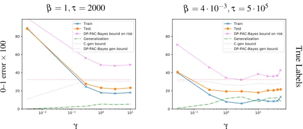
4.6 Numerical evaluations on MNIST . . . 82
4.6.1 Details . . . 83
4.6.2 Results . . . 84
4.7 Two-class MNIST experiments . . . 85
4.7.1 Architecture . . . 85
4.7.2 Training objective and hyperparameters for Entropy-SGLD . . . 86
4.7.3 Evaluating the PAC-Bayes bound . . . 87
4.8 Multiclass MNIST experiments . . . 88
4.8.1 Objective . . . 88
4.9 CIFAR10 experiments . . . 88
4.9.1 Privacy parameter experiments . . . 89
4.9.2 Prior variance experiments . . . 89
4.10 Discussion . . . 90
5 Training GANs with an MMD discriminator 97 5.1 Learning to sample as optimization . . . 98
5.1.1 Adversarial Nets . . . 100 5.1.2 MMD as an adversary . . . 100 5.2 MMD nets . . . 102 5.3 MMD generalization bounds . . . 104 5.4 Proofs . . . 106 5.5 Empirical evaluation . . . 115
5.5.1 Gaussian data, kernel, and generator . . . 115
5.5.2 MNIST digits . . . 115
5.5.3 Toronto Face dataset . . . 116
5.7 Recent Follow-up work . . . 117
Conclusion 119
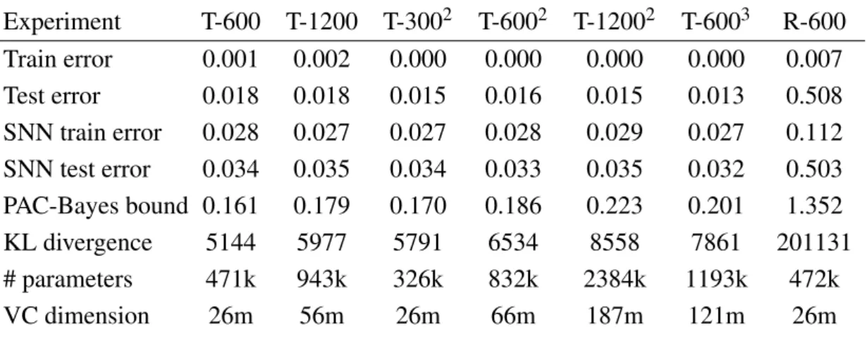
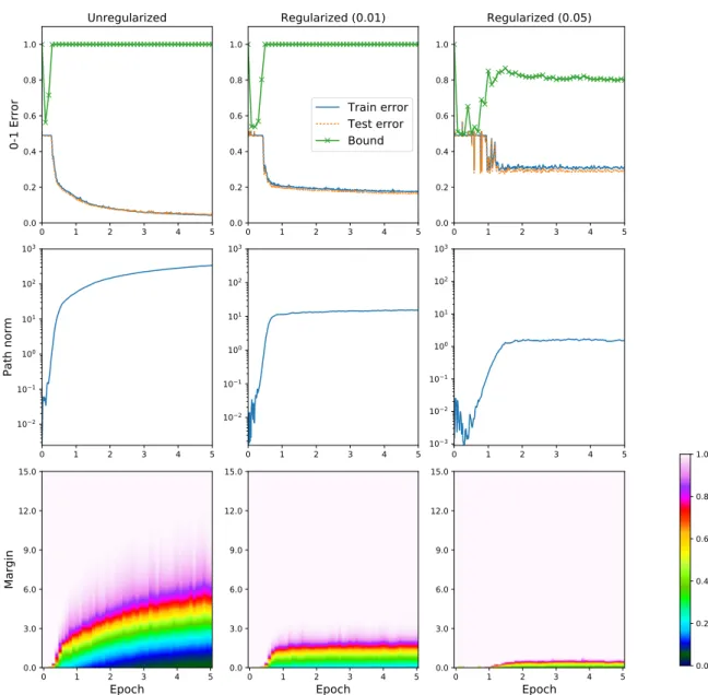
2.1 Rademacher complexity based bounds: tracking path-norm and margin . . . 51
3.1 Generalization bounds with data-dependent priors for MNIST . . . 71
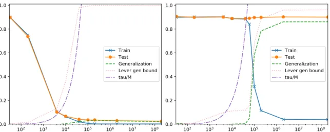
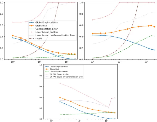
3.2 Comparison of data-dependent PAC-Bayes bounds on a synthetic dataset . . 72
4.1 SGDL and Entropy-SGLD results for various levels of privacy on the CONV network on two-class MNIST. . . 92
4.2 Differentially private Entropy-SGLD results for a fully connected network. 93 4.3 Performance of SGLD when tuned to be differentially private . . . 93
4.4 Entropy-SGLD performance on MNIST . . . 94
4.5 Entropy-SGLD performance on CIFAR10 . . . 95
4.6 Entropy-SGLD CIFAR10 experiments with a fixed level of privacy . . . 96
5.1 Comparison of MMD nets to GANs . . . 99
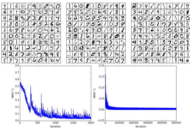
5.2 Samples from MMD nets trained on MNIST. . . 116
N,Z,Q,R naturals, integers, rationals, reals, respectively
M1(S) probability measures on the spaceS
H hypothesis class
ℓ(h,z) loss of a hypothesishon a data pointz
˘
ℓ convex surrogate to the 0–1 loss (logistic loss)
RD(h) risk of a hypothesish
ˆ
RS(h) empirical risk of a hypothesish
I(X,Y) mutual information between two random variablesX andY
ˆ
Rm(S,H ) empirical Rademacher complexity ofH on a datasetS
Rm(H ) Rademacher complexity ofH
kl(q||p) KL divergence between two Bernoulli random variables with probability of successqand p
KL−1(q|c) defined in Eq. (2.1)
Neural networks have enjoyed several waves of popularity. One of the defining properties of the most recent resurgence—the “deep learning” era—is the use of large data sets and much larger networks. Neural network approaches now dominate in fields such as vision, natural language processing, and many others. Despite this success, the generalization properties of deep learning algorithms are yet to be fully understood: there is, as yet, no complete theory explaining why common algorithms work in practice. Instead, guidelines for choosing and tuning common learning algorithm are based on empirical experience. Such practice is problematic. In some applications, standard algorithms like stochastic gradient descent (SGD) reliably return solutions with low test error. In other applications, these same algorithms rapidly overfit.
Our goal is to improve our understanding of generalization of neural networks in the deep learning regime, empowering us to:
1. explain when a learning algorithm can be expected to work well; and 2. design improved algorithms with provable generalization guarantees.
Any attempt to explain generalization must grapple with the fact that the hypothesis class induced by standard neural network models is huge, as measured by standard complexity measures, such as VC dimension and Rademacher complexity. One of the defining properties of deep learning is that models are chosen to have many more parameters than available training data. In practice, the number of available training instances is too small in comparison to the size of the network to yield generalization guarantees without taking into consideration the learning algorithm or depending on the complexity of the learned hypothesis.
This fact has long been appreciated and Bartlett (1998) is essentially credited with solving this problem in 1998. In his seminal work, Bartlett introduced fat shattering risk bounds where the fat shattering dimension of the network is controlled by the norms of the weights. One of the key contributions of this thesis is revisiting this and later developments and questioning whether they solve the problem at hand of understanding generalization in deep learning. One might hope that the generalization properties of SGD could be explained by
showing that SGD performs implicit regularization of the weight norms. However, Bartlett’s learning bounds are numerically vacuous, i.e., greater than the upper bound on the loss, when applied to modern networks learned by SGD. Logically, in order to explain generalization, we need nonvacuous bounds.
Nonetheless, many authors are actively working on understanding implicit regularization and several empirical studies suggest that the implicit regularization idea may be promising (Neyshabur, Tomioka, and Srebro, 2014; Neyshabur, 2017; Zhang et al., 2017; Shwartz-Ziv and Tishby, 2017; Bartlett, Foster, and Telgarsky, 2017a; Gunasekar et al., 2017). For example, Zhang et al. (2017) demonstrate that, without regularization, SGD can achieve zero training error on standard benchmark datasets, like MNIST and CIFAR. At the same time, SGD obtains weights with very small generalization error with the original labels. As a simplified model, Zhang et al. study SGD in a linear model, and show that SGD obtains the minimum norm solution, and thus performs implicit regularization. They suggest a similar phenomenon may occur when using SGD to training neural networks. Indeed, earlier work by Neyshabur, Tomioka, and Srebro (2014) observes similar phenomena and argues for the same point: implicit regularization underlies the ability of SGD to generalize, even under massive overparametrization. Subsequent work by Neyshabur, Tomioka, and Srebro (2015) introduces “path norms” as a better measure of the complexity of ReLU networks. The authors bound the Rademacher complexity of classes of neural networks with bounded path norm. Despite progress, we show that these new bounds probably will not lead to nonvacuous generalization bounds.
The generalization question may also be addressed by studying properties of learning algorithms, such as algorithmic stability. However, existing stability guarantees typically diminish rapidly with training time. The experiments by Neyshabur, Tomioka, and Srebro (2014) demonstrate that the classification error, as estimated on the test set, does not get worse if we run SGD to convergence. On the other hand, Zhang et al. shows that SGD rapidly overfits when handed randomized labels. This example highlights the impediment of using label-independent stability analyses to explaining generalization, as noted by Zhang et al. (2017).
In summary, the theoretical relevance of many learning bounds has been assessed by looking whether the bound captures some implicit regularization, structural properties of the solution, and/or properties of the data distribution. Progress was made by eliminating or improving the dependencies on the number of layers, depth, and parameters in the neural network. Empirical relevance was commonly illustrated via plots that show the generalization bounds tracking the estimated generalization error.
In our work, we take one step further by seeking to obtain generalization bounds that are numerically close to the estimate of generalization on held-out data. Our approach combines Probably Approximately Correct (PAC) Bayes (McAllester, 1999a) framework with nonconvex optimization and other computational techniques. This direction turns out to be fruitful for several reasons. For instance, it yields insight into what empirical risk surface structure found by SGD leads to good generalization and it also allows us to interpret other existing optimizers as risk bound minimizers, analyze and control their generalization guarantees in theory and in practice.
Publications and Collaborations
This thesis brings together a number of results obtained in collaboration with my supervisor Zoubin Ghahramani and Daniel M. Roy. In particular, the main contributions of this thesis appeared in the following publications and preprints:
• Gintare Karolina Dziugaite and Daniel M. Roy (2018a). “Data-dependent PAC-Bayes priors via differential privacy”. Advances in Neural Information Processing Systems (NIPS). vol. 29. Cambridge, MA: MIT Press. arXiv: 1802.09583 (Chapter 3).
• Gintare Karolina Dziugaite and Daniel M. Roy (2018b). “Entropy-SGD optimizes the prior of a PAC-Bayes bound: Generalization properties of Entropy-SGD and data-dependent priors”. Proceedings of the 35th International Conference on Machine Learning (ICML). arXiv: 1712.09376 (Chapter 4).
• Gintare Karolina Dziugaite and Daniel M. Roy (2017). “Computing Nonvacuous Generalization Bounds for Deep (Stochastic) Neural Networks with Many More Parameters than Training Data”. Proceedings of the 33rd Annual Conference on Uncertainty in Artificial Intelligence (UAI). arXiv: 1703.11008 (Chapter 2).
• Gintare Karolina Dziugaite, Daniel M. Roy, and Zoubin Ghahramani (2015). “Train-ing Generative Neural Networks via Maximum Mean Discrepancy Optimization”.
Proceedings of the Thirty-First Conference on Uncertainty in Artificial Intelligence. UAI’15. Amsterdam, Netherlands: AUAI Press, pp. 258–267 (Chapter 5).
The core ideas were developed during discussions with my collaborators Zoubin Ghahra-mani and Daniel M. Roy, and, thus, these contributions are shared among the authors of each of the papers listed above. I carried out all the empirical and theoretical work, with one exception: the results in Section 3.4.1 were derived jointly in collaboration with Daniel M. Roy.
Outline and Contributions
In addition to describing the results appearing in the articles listed above, this thesis contains a more indepth literature review as well as an overview of relevant aspects of statistical learning theory, one of the main tools used in my research.
We start Chapter 1 by formally introducing tools from statistical learning theory that are used for our research. This background material should facilitate the reader in fully understanding the analyses reported in this thesis.
In Chapter 2, we then address the question of nonvacuous generalization bounds for SGD trained networks. We return to an idea by Langford and Caruana (2001), who used PAC-Bayes bounds to compute nonvacuous numerical bounds on generalization error for
stochastic two-layer two-hidden-unit neural networks via a sensitivity analysis. By op-timizing the PAC-Bayes bound directly, we are able to extend their approach and obtain nonvacuous generalization bounds for deep stochastic neural network classifiers with millions of parameters trained on only tens of thousands of examples. We connect our findings to recent and old work on flat minima and MDL-based explanations of generalization.
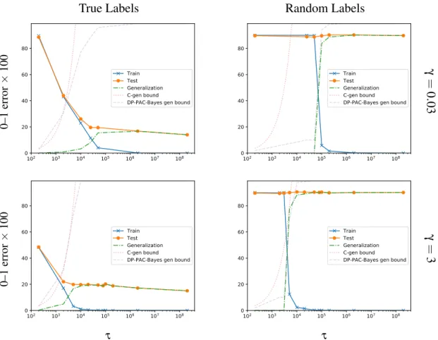
The PAC-Bayes framework can incorporate knowledge about the learning algorithm and data distribution through the use of distribution-dependent priors, yielding tighter gener-alization bounds on data-dependent posteriors. Using this flexibility, however, is difficult, especially when the data distribution is presumed to be unknown. In Chapter 3 we show how anε-differentially private choice of the prior yields a valid PAC-Bayes bound, and then show how non-private mechanisms for choosing priors obtain the same generalization bound provided they converge weakly to the private mechanism. As a consequence, we show that a Gaussian prior mean chosen via stochastic gradient Langevin dynamics (SGLD; Welling and Teh, 2011) leads to a valid PAC-Bayes bound, despite SGLD only converging weakly to anε-differentially private mechanism. As the bounds are data-dependent, we use empirical results on standard neural network benchmarks to illustrate the gains of data-dependent priors over existing distribution-dependent PAC-Bayes bound.
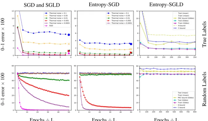
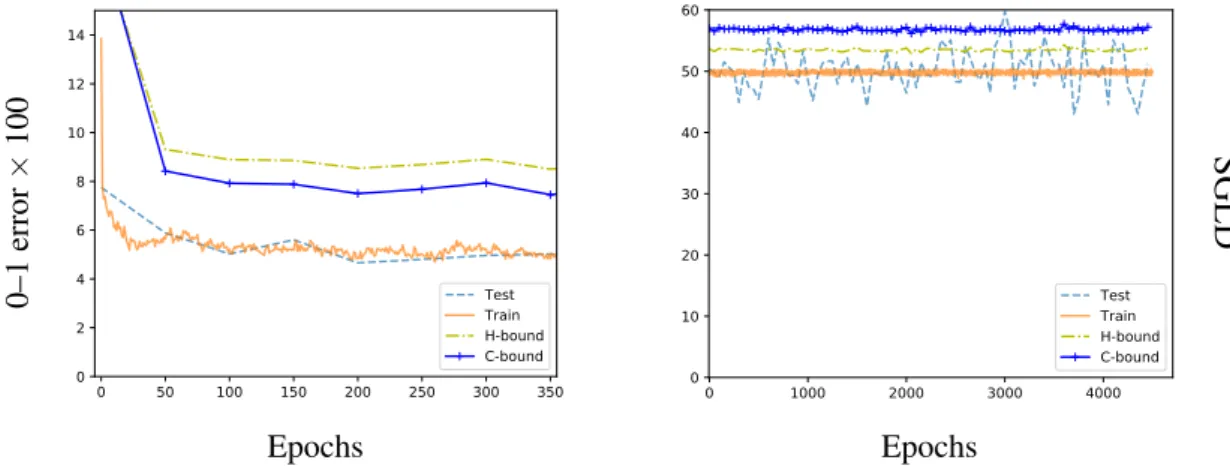
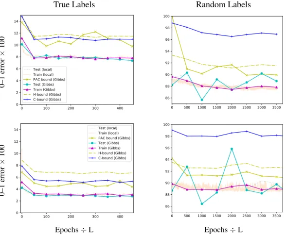
In Chapter 4, we show that Entropy-SGD (Chaudhari et al., 2017), when viewed as a learning algorithm, optimizes a PAC-Bayes bound on the risk of a Gibbs (posterior) classifier, i.e., a randomized classifier obtained by a risk-sensitive perturbation of the weights of a learned classifier. Entropy-SGD works by optimizing the bound’s prior, violating the hypothesis of the PAC-Bayes theorem that the prior is chosen independently of the data. Indeed, available implementations of Entropy-SGD rapidly obtain zero training error on random labels and the same holds of the Gibbs posterior. In order to obtain a valid generalization bound, we rely on our result showing that data-dependent priors obtained by SGLD yield valid PAC-Bayes bounds. We observe that test error on MNIST and CIFAR10
falls within the (empirically nonvacuous) risk bounds computed under the assumption that SGLD reaches stationarity. In particular, Entropy-SGLD can be configured to yield relatively tight generalization bounds and still fit real labels, although these same settings do not obtain state-of-the-art performance.
In Chapter 5, we consider training a deep neural network to generate samples from an unknown distribution given i.i.d. data. We frame learning as an optimization minimizing a two-sample test statistic—informally speaking, a good generator network produces samples that cause a two-sample test to fail to reject the null hypothesis. As our two-sample test statistic, we use an unbiased estimate of the maximum mean discrepancy, which is the centerpiece of the nonparametric kernel two-sample test proposed by Gretton et al. (Gretton et al., 2012). We compare to the generative adversarial nets framework introduced by Goodfellow et al. (Goodfellow et al., 2014), in which learning is a two-player game between a generator network and an adversarial discriminator network, both trained to outwit the other. From this perspective, the MMD statistic plays the role of the discriminator. In addition to empirical comparisons, we prove bounds on the generalization error incurred by optimizing the empirical MMD.
Statistical Learning Theory
In this chapter we introduce basic concepts from statistical learning theory. Informally, learning uses data to improve performance on one or more tasks. Statistical learning theory provides a formal framework for defining learning problems, measuring their complexity, and anticipating the performance of learning algorithms.
In this section, our focus will be on the batch supervised learning setting, and, in particular, classification. In supervised learning, we want to learn a mapping from a space
Rk of inputs to a spaceKof labels. The goal is to find the best predictor, or hypothesis, h,
in some hypothesis classH ⊆Rk→K, on the basis of example input–output pairs. In the batch setting, these examples are presented all at once to the learner and are assumed to be independent and identically distributed (i.i.d.).
In the batch setting, the i.i.d. assumption allows us to link (past) empirical performance to (future/expected) performance. Empirical performance is thus a key measure of the quality of a proposed hypothesis. However, empirical performance can be misleading, depending on the quantity of data and the learning algorithm. Generalization bounds relate empirical performance to performance on unseen data, and can give us confidence using a learning algorithm. These bounds may depend on a number of factors, including:
1. the hypothesis class the learner is considering (Section 1.1.3); 2. the underlying data distribution (Section 1.1.3);
3. the properties of the chosen predictor and/or prior knowledge expressed by the learner (Section 1.2);
4. the properties of the algorithm used by the learner (Sections 1.3 and 1.4), such as its stability, the property that the distribution of the algorithm’s output does not change when small modifications are made to the training data.
Bounds that depend only on (1) exist, but they capture only worst-case scenarios. Taking the data distribution into considerations often yields tighter bounds. Bounds combining all factors listed above are specific to the particular problem being studied and yield the tightest known bounds.
1.1
Supervised learning
LetZbe a measurable space, and letD be an unknown distribution onZ. Consider the batch supervised learning setting under a loss function bounded below: having observedS∼Dm, i.e.,mindependent and identically distributed samples fromD, we aim to choose a predictor belonging to some hypothesis classH and parameterized by a weight vectorw∈Rp, with minimalrisk
RD(w):= E
z∼D(ℓ(w,z)), (1.1)
where ℓ:Rp×Z →R is measurable and bounded below. (We ignore the possibility of constraints on the weight vector for simplicity.)
We will also consider randomized predictors. A randomized predictor is represented by an elementQin the spaceM1(Rp)of probability measure onRp. The risk of randomized
predictors is defined via averaging:
RD(Q):= E w∼Q(RD(w)) =z∼ED E w∼Q(ℓ(w,z)) , (1.2)
where the second equality follows from Fubini’s theorem and the fact that ℓ is bounded below.
Let Sm= (z1, . . . ,zm)denote a training set of size m. We will often drop the subscript
mand simply write S, unless the training set size is not obvious. Let ˆD := m1∑mi=1δzi be
the empirical distribution. Given a weight distributionQ, such as that chosen by a learning algorithm on the basis of dataS, itsempirical risk,
ˆ RS(Q):=RDˆ(Q) = 1 m m
∑
i=1 E w∼Q(ℓ(w,zi)), (1.3) will be studied as a stand-in for its risk, which we cannot compute. While ˆRS(Q)is easily seen to be an unbiased estimate ofRD(Q)whenQis independent ofS, our goal is to characterize the (one-sided)generalization error RD(Q)−RˆS(Q)whenQis random and dependent onS. Note, that throughout this thesis, we will often use a term generalization bounds, by which we refer to a bound on the difference between the risk and empirical risk.1.1.1
Loss functions
One of our focuses will be on classification, where Z =X ×K, with K a finite set of classes/labels. A product measurable function h:Rp×X →K maps weight vectors wto classifiersh(w,·):X→K. The loss function is given byℓ(w,(x,y)) =g(h(w,x),y)for some
g:K×K→R. In this setting, 0–1 loss corresponds tog(y′,y) =1 if and only ify′̸=y, and otherwiseg(y′,y) =0. In binary classification, we takeK={−1,1}. Thus, under 0–1 loss
ℓ:Rp×(X,K)→ {0,1}satisfies
ℓ(w,(x,y)) =I(sign(h(w,x))̸=y).
In Chapter 2, forK={±1}, we also make use of the logistic loss ˘ℓ:Rp×(X,{±1})→R+
˘
ℓ(w,(x,y)) = 1
log(2)log 1+exp(−h(w,x)y)
,
which serves as a convex surrogate (i.e., upper bound) to the 0–1 loss.
We also consider parametric families of probability-density-valued classifiersh:Rp×
X →[0,1]K. For every inputx∈X, the outputh(w,x)determines a probability distribution on K. In this setting,ℓ(w,(x,y)) =g(h(w,x),y)for someg:[0,1]K×K→R. The standard loss is then the cross entropy, given byg((p1, . . . ,pK),y) =−logpy. (Under cross entropy loss, the empirical risk is, up to a multiplicative constant, a negative log likelihood.) In the special case of binary classification, the output can be represented simply by an element of [0,1], i.e., the probability the label is one. The binary cross entropy,ℓBCE, is given by
g(p,y) =−ylog(p)−(1−y)log(1−p). Note that cross entropy loss is merely bounded below. We consider bounded modifications in Section 4.7.2.
In the context of supervised learning, we will sometimes refer to elements ofRp and
M1(Rp)as classifiers and randomized classifiers, respectively. Likewise, under 0–1 loss, we
will sometimes refer to (empirical) risk as (empirical) error.
In summary, we define the following notions of risk that we use throughout: • ˆRS(w) = 1
m
m
∑
i=1ℓ(w,zi) empirical risk of (hypothesis indexed by parameters) w on training dataS(under 0–1 loss, training error);
• ˘RS(w) = 1 m m
∑
i=1 ˘ℓ(w,zi)empirical risk under the surrogate loss (or surrogate error) ofw on training dataS. We use this empirical risk for training purposes in Chapter 2 when we need our objective to be differentiable;
• RD(w) = E S∼Dm[
ˆ
Rw(S)]risk (error) under (the data distribution)D forw(in Chapter 2, we often drop the subscriptD and just writeR(w));
• ˆRS(Q) = E w∼Q[
ˆ
RS(w))]empirical risk (error) of (randomized classifier)Qon training dataS;
• R(Q)) = E
w∼Q[RD(w)]risk (error) ofQunderD
1.1.2
Empirical risk minimization and PAC-learning
In the rest of this section, we introduce basic principles from statistical learning theory. This development mirrors the development in the book of Shalev-Shwartz and Ben-David (2014).
Empirical risk minimization (ERM) is an idealized learning algorithm that chooses the parametersw∗whose risk matches the best possible risk
inf w∈H
ˆ
RS(w). (1.4)
The properties of ERM are well studied. A large hypothesis class H may contain a predictor with minimal empirical risk but large true risk, leading to a high generalization error, i.e.,overfitting. Choosing a more restrictive hypothesis class may prevent overfitting in exchange for bias. Sharp results exist relating the possibility of obtaining uniform bounds on the generalization error to properties of the hypothesis classH and the 0–1 loss functionℓ.
Definition 1.1.1(Agnostic PAC Learnable). Let an algorithm map a training sample to a hypothesis, i.e.,A : Zm→H . A hypothesis classH is called(agnostic) PAC learnable
if there exists an algorithmA and a functionmH(ε,δ):(0,1)2→N, such that for every (ε,δ)∈(0,1)2 and a data distribution D, for all m>mH(ε,δ), with probability at least 1−δ over the training sampleS,
RD(A(S))≤ min w∈H
RD(w) +ε. (1.5)
We callmH(ε,δ)asample complexityforH , i.e., it is the number of examples needed to guarantee PAC learnability ofH.
In other words, if a PAC learning algorithm is given enough data, for any data distribution it is guaranteed with high probability to return a predictor that is nearly as good as the best predictor in the hypothesis class. It is also known that aH is PAC learnable if and only if it is learnable by ERM.
Uniform convergence
There are many ways to understand PAC learnability, one of the key ways is through uniform convergence. This property guarantees that our generalization error converges to zero with the sample size, and quantifies the rate of that convergence.
Definition 1.1.2(Uniform Convergence). A hypothesis classH has theuniform convergence
(UC) property if there exists a functionmUCH (ε,δ):(0,1)2→N, such that for every(ε,δ)∈ (0,1)2 and data distributionD, for allm≥mUCH (ε,δ), with probability at least 1−δ over the training sampleS,
RD(w)−RˆS(w) ≤ε. (1.6)
We define the sample complexity ofH to be the smallest function m satisfying the definition ofmUCH .
A fundamental result in statistical learning is that a class is PAC learnable if and only if it has the UC property.
1.1.3
Bounding the sample complexity: VC dimension and Rademacher
complexity
Hypothesis classes with the UC property vary in terms of their sample complexity. Here we introduce two ways to measure the complexity of the hypothesis class that allows us to bound the sample complexity.
VC dimension
One measure of complexity of the hypothesis class is expressed in terms of the number of ways it can label the dataset.
Definition 1.1.3(Shattering). LetH be a class of binary predictors parametrized byw, i.e., eachw∈H mapsX toK={0,1}. LetXm={x1, ...,xm} ∈Xm. ThenH is said to shatter
Xmif
{(h(w,x1), ..,h(w,xn)):w∈H } ⊇ {0,1}m (1.7)
Definition 1.1.4(VC dimension). The VC dimension of a binaryH , denoted by VCdimH, is the maximum size of a set that it can shatter.
Thus ifH has VC dimensiond, we know that there is a hypothesiswin the class that achieves zero empirical risk for every labelling of some dataset of sized. A key result in statistical learning is thatH has uniform convergence property if and only if it has a finite VC dimension.
The VC dimension can be used to bound the sample complexity, and thus the general-ization error. However, VC bounds on the generalgeneral-ization error are loose in practice as they account for worst case data distributions. These bounds are valid for any data distribution
D and any ERM learning algorithm, and thus it needs to give a bound that holds for an adversarially crafted hypothesis for the data distribution.
One can bound the VC dimension of neural network hypothesis space. The first bounds in the literature are reported in (Goldberg and Jerrum, 1995; Koiran and Sontag, 1996) and depend on the number of parameters in the network. Bartlett, Maiorov, and Meir (1999) improved these bounds by introducing the dependence on the number of layers. These bounds are of orderO(LWlog(W), whereW is the number of parameters in the neural networks and
Lis the number of layers. In Chapter 2 we evaluate one of such bounds and show that for large neural networks used in practice, we get a very large upper bound on the VC dimension (more than 107). The large VC dimension combined with a relatively small number of training examples in the dataset results in generalization bounds that are orders of magnitude too big to make a nonvacuous guarantee on the risk.
Rademacher Complexity
The VC bounds discussed above ignore the distribution over the data. Thus one can possibly get tighter bounds by incorporating the data distribution. In this section, we describe the application ofRademacher complexity to statistical learning theory (Koltchinskii and Panchenko, 2002; Bartlett and Mendelson, 2003).
Definition 1.1.5(Rademacher Complexity). Fix a sample sizem∈N. Letσ ={σi}i∈Nbe a
sequence ofRademacher random variables, i.e., random variables taking values in{−1,1}
with equal probability. Fix a class of measurable functionsF ⊆Z→R. For a sampleS∈Zm, the empirical Rademacher complexity of the classF is
ˆ Rm(S,F) =Eσ[sup f∈F 1 m m
∑
i=1 σifi(zi)]. (1.8)The Rademacher complexity (under a data distributionD) of the classF is
Usually, one studies the Rademacher complexity of the loss class, and thusF refers to the loss function composed withH , i.e., all f ∈F are such that f(x,y) =ℓ(w,(x,y))for somew∈H . In this case, the Rademacher complexity can be used to obtain the mean of worst case generalization error:
Theorem 1.1.6. E S∼D h sup w∈Rp RD(w)−RˆS(w)i≤2Rm({ℓ(w,·):w∈Rp}) (1.10)
This bound can be used to prove a bound on the expected generalization error and expected oracle risk (the gap between risks of an ERM classifier and the best classifier in the hypothesis class) of any ERM mechanism.
One of the key application of Rademacher complexity in statistical learning theory is to margin bounds for classifiers that output a real-valued prediction. The 0-1 loss of these predictors is obtained by thresholding the output. To obtain a margin bound, one studies the ramp loss, a Lipschitz upper bound to the 0–1 loss. One can show that the Rademacher of the loss class is no larger than the product of the Lipschitz constant and the Rademacher complexity of the real-valued hypothesis class. In this case, theH has a high Rademacher complexity if it is rich enough to contain predictors that can explain a random labelling of the data.
In Chapter 2 we present and evaluate a generalization error bound for neural network classifiers. Also, in Chapter 5 (Section 5.4), we introduce a neural network generative model and use the Rademacher complexity to obtain some generalization guarantees.
1.1.4
Structural Risk Minimization
The method of ERM finds a hypothesis minimizing the empirical risk. However, for very complex hypothesis classes, ERM may lead to overfitting: low empirical risk does not guarantee low risk. One solution is to introduce more structure in the hypothesis class that reflects the varying complexity of the hypothesis within the original hypothesis class. This is exactly the motivation behindStructural Risk Minimization, which was introduced by Vapnik and Chervonenkis (1974).
Fix a hypothesis classH, letSbe a dataset, and consider a bound on the risk of the form
αRˆS(w) +C(w), (1.11)
whereα ∈R+ and the termC(w)may depend on the hypothesisw. In ERM, the termC(w) is a constant, i.e., it does not depend on the particular hypothesisw. In classical SRM, the
termC(w)is not constant, and so Eq. (1.11) encodes a trade-off between the empirical risk and some notion of complexity for predictors.
Consider a hypothesis classH = S n∈N
Hn where, for eachn∈N, the subclassHnhas the uniform convergence property with sample complexitymUCH
n(ε,δ). Define the function
εn:M ×N×(0,1)→(0,1)as
εn(m,δ) =min{ε ∈(0,1):mUCHn(ε,δ)≤m}. (1.12) Define a weight functionw:N→[0,1]over each hypothesis class{Hn}n∈NinH, such that
∑n∈Nw(n)≤1. The following generalization guarantee holds:
Theorem 1.1.7. (Shalev-Shwartz and Ben-David, 2014) LetH , w, and εn be defined as
above. Then for allδ ∈(0,1)andD, for allw∈H , with probability at least1−δ over the
choice of S,
RD(w)≤RˆS(w) + min n:w∈Hn
εn(m,δ·w(n)). (1.13) Note that, the weight function, once normalized, has the same form as a prior distribution in Bayesian analysis. However, the guarantee holds for any weight function, provided it is fixed before seeing the data. The theorem makes it clear that we are incentivized to assign large weight to small subclassesHnthat we believe will fit the data well, and so there is an indirect link with the Bayesian prior.
The risk bound, Eq. (1.13), suggests a natural learning algorithm for any hypothesis space that can be written as a countable union of PAC learnable classes. The following paradigm is called Structural Risk Minimization (SRM):
1. WriteH = S n∈N
Hnfor some countable collection of PAC learnable subclasses; 2. Assign weightw(n)to eachHn, with∑nw(n)≤1;
3. Given dataSand a confidence parameterδ ∈(0,1), choosew∈H that minimizes the right hand side of Eq. (1.13).
It is common to use a VC bound onεn(w)(m,δw(n(w))).
Nonuniform learnabilityis a weaker notion than PAC learnability. The latter implies the former. In PAC learnability one is required to choose a single value for sample complexity
mH(ε,δ)that works uniformly for all hypothesis inH (including the hypothesis that has the lowest true error). Nonuniform learnability relaxes this requirement by allowing to setm
Note, that while each hypothesisHnin SRM is uniformly learnable,H is only nonuni-formly learnable.
The SRM paradigm drives the learning towards the simplest hypothesis that achieves a relatively low empirical risk. This closely connects to the Minimum Description Length (MDL) and PAC-Bayes frameworks discussed in the following sections.
1.1.5
Minimum Description Length
The Minimum Description Length (MDL) principle can be seen as a special case of SRM. In MDL:
• eachHnis a singleton class. ByHoeffding’s inequality,εn(m,δ)decays as 1/
√
m; • the weightsw(n)of eachHnare assigned based on an information-theoretic notion of
complexity, namely the description length of a hypothesis. In MDL, the learning task is viewed as a compression task.
See Grünwald (2005) for a tutorial and further references on MDL. The article also discusses how MDL connects to Bayes factor model selection and Bayesian inference. In Chapter 2 we mention how MDL connects to PAC-Bayes.
1.2
PAC-Bayes
PAC-Bayes theory was first developed by McAllester in 1999 with the goal to provide PAC learning guarantees for Bayesian algorithms. The first PAC analysis of Bayesian algorithms is due to Shawe-Taylor and Williamson. The developed theory reported in (Shawe-Taylor and Williamson, 1997) apply under more restrictive set of assumptions on the parameter space and prior measures, as compared to McAllester’s work.
PAC-Bayes theorems give generalization and oracle bounds that can be used to build and analyze learning algorithms that are similar to SRM and MDL. In all three settings, the learner:
• fixes a prior/weight function over the hypothesis class, prior to seeing the data; • optimizes a bound on the risk of the form Eq. (1.11).
The prior can also be interpreted as a data-independent randomized classifer.
Unlike in SRM or MDL, PAC-Bayes bounds are generally used to control the risk of data-dependentrandomizedclassifiers. PAC-Bayes bounds lead to a natural variant of SRM where:
• as in MDL, the hypothesis classH = S
h∈H Hhis viewed as a (possibly uncountable)
union of singleton classesHh={w};
• the weight function in MDL is replaced by a (possibly atomless) probability measure
PoverH ;
• the search over classifiers,h, is replaced by one overrandomizedclassifiers,Q, i.e., probability measures overH
MDL is obtained as the special case whereH is countable and the search is restricted to degenerate probability measures (i.e., ones assigning probability one to a single hypothesis). Note thatPandQare the same type of structure.
1.2.1
KL divergence and the PAC-Bayes theorem
Let Q,P be probability measures defined onRp, assumeQis absolutely continuous with respect toP, and write ddQP :Rp→R+∪ {∞}for some Radon–Nikodym derivative ofQwith respect toP. Then the Kullback–Liebler divergence (or relative entropy) of PfromQis defined to be
KL(Q||P):=
Z
logdQ
dPdQ. (1.14)
We are mostly concerned with KL divergences whereQandPare probability measures on Euclidean space,Rd, absolutely continuous with respect to Lebesgue measure. Letqand p
denote the respective densities. In this case, the definition of the KL divergence simplifies to KL(Q||P) =
Z
logq(x)
p(x)q(x)dx.
Of particular interest to us is the KL divergence between multivariate normal distributions inRd. LetNq=N (µq,Σq)be a multivariate normal with meanµqand covariance matrix
Σq, letNp=N (µp,Σp), and assumeΣqandΣpare positive definite. Then KL(Nq||Np)is 1 2 tr Σ−p1Σq −k+ µp−µq⊤Σ−p1(µp−µq) +ln detΣp detΣq . (1.15)
For p,q∈[0,1], we abuse notation and define kl(q||p):=KL(B(q)||B(p)) =qlogq p+ (1−q)log 1−q 1−p,
whereB(p)denotes the Bernoulli distribution on{0,1}with mean p.
1.2.2
Bounds
We now present a PAC-Bayes theorem, first established by McAllester (1999a). We focus on the setting of bounding the generalization error of a (randomized) classifier on a finite discrete set of labelsK. The following variation is due to Langford and Seeger (2001) for 0–1 loss (see also (Langford, 2002) and (Catoni, 2007).)
Theorem 1.2.1(PAC-Bayes (McAllester, 1999a; Langford and Seeger, 2001)). Under 0–1 loss, for everyδ >0, m∈N, distributionD onRk×K, and distribution P onRp,
P S∼Dm (∀Q)kl(RˆS(Q)||RD(Q))≤ KL(Q||P) +log2m δ m−1 ≥1−δ. (1.16) The application of PAC-Bayes bounds to learning algorithms is the following: pick a randomized classifierPbefore seeing the data, which is your prior; the learning algorithm chooses a randomized classifierQbased on the data; then with high probability,Qwill have small risk if Qhas small empirical risk and the KL divergence betweenQand Pis small relative to the number of data points.
We also use the following variation of a PAC-Bayes bound, where we consider any bounded loss function.
Theorem 1.2.2(Linear PAC-Bayes Bound (McAllester, 2013; Catoni, 2007)). Fixλ >1/2
and assume the loss takes values in an interval of length Lmax. For every δ >0, m∈N,
distributionD onRk×K, and distribution P onRp,
P S∼Dm (∀Q)RD(Q)≤ 1 1−21 λ ˆ RS(Q) +λLmax m (KL(Q||P) +log 1 δ) ≥1−δ. (1.17)
1.2.3
Optimal Prior and Posterior
AGibbs posterior(for a priorP) is a distribution that is absolutely continuous with respect to
literature, the parameterτ is referred to asinverse temperature. Gibbs distributions arise as the solutions of various optimization problems.
Gibbs posterior as the optimal posterior
Fix a prior distribution P. It is well known that the optimal data-dependent randomized classifierQthat minimizes the PAC-Bayes risk bound is a Gibbs posterior. The result appears in McAllester (2003, Thm. 2) for a PAC-Bayes bound that is valid for any measurable loss functions, but the hypothesis class is restricted to be finite. A more general result for uncountableH was developed by Catoni (2007, Lem. 1.1.3) in the case of bounded risk.
Thus for a givenPand a bounded loss function, the optimal distributionQminimizing the linear PAC-Bayes bound satisfies
dQ dP(w) = exp(−τRˆS(w)) R exp(−τRˆS(w))p(dw) . (1.18)
For someτ,λ in the linear PAC-Bayes bound stated in Theorem 1.2.2 can be expressed in terms of the inverse temperature parameterτ.
Local Priors
It is natural to consider a fixed data-dependent posterior Q=Q(S) and ask what prior optimizes a PAC-Bayes bound. Catoni (2007) studied this question and showed that the optimal prior (in expectation) is
P= E
S∼D[Q(S)]. (1.19)
This prior is not available in practice because we do not know D. Instead, one can study some non-optimal but data-distribution-dependent prior distributions.
In the case whenQ(w)is a Gibbs classifier with density proportional to
e−τRˆS(w)−γFQ(S,w), (1.20)
Lever, Laviolette, and Shawe-Taylor (2013) were able to bound the KL divergence with a distribution-dependent prior whose prior density is
While this prior choice is not optimal, it is an interesting case to study due to optimality of Gibbs distributions discussed above. The functions FQ and FP may be different and act as regularizers. They may depend on the parameters of the hypothesis or perform a data-dependent regularization. In (Lever, Laviolette, and Shawe-Taylor, 2013), the authors give localized PAC-Bayes bounds for these particular choices ofPandQ.
The use of an informed prior gives a much tighter Bayes bound. A generic PAC-Bayes bound depends on KL(Q||P). This term may be very large whenPis chosen poorly and is not tailored for the specific task at hand. In the analysis presented by Lever, Laviolette, and Shawe-Taylor (2013), they eliminate the KL term by replacing it with an upper bound whenPandQare chosen as described above. In Chapter 3 we study local prior bounds and develop a new data-dependent prior bound that depends on the properties of the algorithm used to chooseP.
For a use of local priors, see, e.g., Parrado-Hernández et al. (2012). In this work, the authors provide tighter PAC-Bayes generalization bounds for SVM classifiers. They explore several strategies to achieve this. One idea is to use part of the dataset to learn a better prior for a PAC-Bayes bound, which the authors call a prior PAC Bayes bound. Another idea is to choose a Gaussian prior with the mean depending on the data distribution. Since the data distribution is not available, the authors instead use an empirical data distribution and then upper bound the difference between the expected parameter value under the empirical distribution and the true data distribution. This approach yields a bound named an expectation prior PAC-Bayes bound (Parrado-Hernández et al., 2012, Thm. 9). Their experiments demonstrate that the use of informative priors for SVM classifiers results in tighter PAC-Bayes bounds.
1.2.4
Gibbs posteriors in (generalized) Bayesian Inference
In Section 1.2.3 we introduced Gibbs distributions and discussed how they relate to PAC-Bayes generalization bounds. In this section we discuss other optimality properties of Gibbs distributions.
Bissiri, Holmes, and Walker (2016) introduce “general Bayesian updating”, a framework that generalizes the classical Bayesian inference by replacing the negative log likelihood in the Bayesian update of the posterior with a more general loss function.
More precisely, ifP(w)represents your prior beliefs about the parametersw, then for some loss function and the corresponding empirical risk ˆRS(w)on the observed dataS, the
general Bayesian posterior is proportional to
e−mRˆS(w)P(w). (1.22)
This is equivalent to Eq. (1.18) with a rescaled loss function, i.e., the density of a Gibbs posterior withτ=m. In a special case, where the loss function is the negative log likelihood andτ =m, the term−τRˆS(w)is the expected log likelihood underQ. This demonstrates the connection among the PAC-Bayes optimal posteriors, general Bayesian inference, and classical Bayesian inference. However, note that the latter works under an assumption that the likelihood contains the true data generating distribution. In contrast, the former frameworks are valid under model misspecification. Most PAC-Bayes generalization bounds require a bounded loss function. Germain et al. (2016) study the connection between PAC-Bayes and Bayesian inference and extend PAC-Bayes generalization bounds for regression tasks and real-valued unbounded loss functions. Similar connections have been made by Zhang (2006a), Zhang (2006b), Jiang and Tanner (2008), Grünwald (2012), and Grünwald and Mehta (2016).
The log normalizing constant of a Gibbs posterior is log
Z
exp(−τRˆS(w′))P(dw′). (1.23)
In the thermodynamics literature, this is anentropy. We encounter a local version of the entropy in Chapter 4 when we study Entropy-SGD. The entropy also arises in minimax regret analysis (Yamanishi, 1998; Yamanishi, 1999). There it is known as the extended stochastic complexity (ESC; Yamanishi 1999). The ESC is applied to both batch and online learning. For online learning algorithms, it can be shown that ESC minimizes the so-called worst case regret.1 The ESC also asymptotically achieves minimax estimation error.2 In Yamanishi (1999) ESC upper bounds the so-called Relative Cumulative Loss for an online learning algorithm. The Relative Cumulative Loss is the difference between the accumulated loss achieved by the online learning algorithm and the minimal accumulated empirical loss for the best hypothesis in the class (empirical risk times the number of examples). See (Yamanishi, 1998; Yamanishi, 1999) for more details. Yamanishi also connects his work to MDL and generalized Bayesian inference.
1The worst case regret is defined as the maximum difference between cumulative logarithmic loss of the online learning algorithm and the minimum cumulative logarithmic loss achievable by someh∈H.
2The estimation error here is slightly different from the one defined in the beginning of the chapter and is adapted for online learning algorithms. Bounds on estimation error are also often referred to as excess risk or oracle bounds.
1.2.5
PAC-Bayes risk bound as an optimization objective
Variational InferenceBayesian inference employs Bayes rule to express a posterior distribution over the hypothesis class. In most but the simplest scenarios, this distribution is computationally intractable. One can target this problem by building approximate samplers for the posterior distribution (MCMC methods). An alternative approach is provided by variational methods.
In variational Bayesian inference, one replaces the exact inference problem, with an approximate one. The approximate inference problem can then be angled as an optimization problem.
The density of the Bayesian posterior measureQBayeson the hypothesis space is given by
p(w|S) =R p(w,S)
p(w,S)dw. (1.24)
The integral in the denominator is the marginal density of the observationsS, also called the evidence. The evidence is intractable for many models of interest. In variational inference, the goal is to find a distribution close to the Bayesian posterior QBayes. We can formalize
this as finding a distributionQVI(with densityq(w)) within a tractable family of probability
measuresQsatisfying
QVI=arg min Q∈Q
KL(Q||QBayes). (1.25)
Computing this KL term is intractable. However, the optimization problem can be seen to be equivalent to QVI=arg max Q∈Q logp(S)−KL(Q||QBayes) (1.26) =arg max Q∈QE[log p(w,S)]−E[logq(w)] (1.27) =arg max Q∈QE [logp(S|w)]−KL(q(w)||p(w)). (1.28)
The objective in Eq. (1.28) is called the evidence lower bound objective (ELBO). In modern stochastic variational inference, one then proceeds by using stochastic gradient method to optimize the ELBO objective and findQVI. For a review on variational inference methods,
see, e.g., Blei, Kucukelbir, and McAuliffe (2017).
The first term in the ELBO objective is the expected log likelihood, which is unknown. During optimization, it is usually replaced with its Monte Carlo estimate. Thus in variational
inference, we optimize the parameters ofQto maximize ˆ
RS(Q)−βKL(Q||P). (1.29)
for some priorP. The reader may recognize that the ELBO objective is of the same form as Eq. (1.11), and, in particular, a linear PAC-Bayes bound on the risk (Theorem 1.2.2), with the loss chosen to be log loss. The connection between minimizing PAC-Bayes bounds under log loss and maximizing log marginal densities is the subject of recent work by Germain et al. (2016).
Kingma, Salimans, and Welling (2015) use variational inference to improve the dropout technique in neural network training. The original Gaussian dropout (Srivastava et al., 2014) can be interpreted as sampling stochastic weights. The sampling distribution is isotropic gaussian, centered at the current weight values, with variance equal to the dropout rate (and thus the variance is equal for all weights in the network). Kingma, Salimans, and Welling (2015) treat the dropout rate as a variational parameter which is learned via optimization.
In summary, the variational dropout can be interpreted as optimizing the parameters ofQ
by minimizing a PAC-Bayes risk bound with a fixed prior. The posterior distribution on the parameters is a stochastic classifierQ, which is an isotropic Gaussian with variances tuned to the individual weights. This closely resembles our work presented on PAC-Bayes risk bound optimization and described in Chapter 2.
1.3
Algorithms and Stability
An algorithm is uniformly stable if its output is relatively insensitive to a change in the input. This notion of stability is fairly strong as it is independent of the data distribution and thus has to account for the worst case scenarios and very unlikely draws of the training data. Uniform stability of a learning algorithm allows one to bound the performance of the classifier returned by the algorithm.
Definition 1.3.1(Uniform Stability; Bousquet and Elisseeff 2002). An algorithm A isε -uniformly stable with respect to a loss functionℓif, for all pairsS,S′∈Zmthat differ at only one coordinate, we have ˆRS(A(S))−RˆS(A(S′))≤
ε.
Note, that uniform stability depends on the dataset sizemand requires the algorithm to be deterministic. One can easily extend this to randomized algorithms and obtain generalization in expectation. See (Hardt, Recht, and Singer, 2015) for more details.
We can relate stability to concentration bounds using a method of bounded differences. In particular, using McDiarmid’s inequality, it is fairly straightforward to get a generalization bound for an output of a uniformly stable algorithmA.
Theorem 1.3.2(McDiarmid’s Inequality (Mendelson, 2003)). Let s1, ..,smbe random vari-ables, and S= (s1, ..,sm). Assume vectors S and Sidiffer at only one coordinate i. Let a function F map S toR. Then if there exists(c1, ...,cm), such that F satisfies
sup S,S′
|F(S)−F(S′)| ≤ci (1.30)
for all i∈ {1, ...,m}, then for allε>0
P |F(S)−E S[F(S)]|>ε ≤exp −2ε2 ∑Nn=1c2n . (1.31)
Now considerF(S) =R(A(S))−RˆS(A(S)). Then it is straightforward to show that
E
S[F(S)]is bounded byε. Assume that the loss functionℓis bounded and takes values in an interval of lengthLmax. Then we can easily demonstrate that|F(S)−F(S′)|is bounded in terms ofε andLmax. It is a straightforward exercise to apply McDiarmid’s inequality to F to
get a bound on|F(S)−E
S[F(S)]|, and a bound on the risk follows.
Theorem 1.3.3(Uniform stability implies generalization; Bousquet and Elisseeff 2002). Let an algorithmA beε−uniformly stable. Assume the loss function takes values in an interval
of length Lmax. Then with probability at least1−δ over the training sample S,
R(A(S))≤RˆS(A(S)) +2ε+ (2mε+Lmax)log
1
δ
2m . (1.32)
There exists a number of other notions of stability, that either imply generalization with high probability, or in expectation. For a comparison, see, e.g. Bousquet and Elisseeff (2002) and Bassily et al. (2016).
1.3.1
Stochastic Gradient Descent
The workhorse of modern machine learning is stochastic gradient descent (SGD). In the context of supervised learning, SGD iteratively takes steps along unbiased (though, in practice, correlated) estimates of the gradient of a risk for a differentiable loss function l.
More concretely, given an initial hypothesisw0∈Rp, SGD repeatedly performs the updates wn+1=wn−ηn1 k k
∑
i=1 ∇wnℓ(wn,zji) (1.33)where, on each roundn=1,2, . . ., some numberk<mindices j1, . . . ,jkare chosen uniformly at random and without replacement from[m]:={1,2, . . . ,m}.
1.3.2
Stability of SGD
In a recent paper by Hardt, Recht, and Singer (2015), the authors show that under some regularity conditions on the loss function and its gradients, SGD is anε−uniformly stable algorithm. Theε decays at the rate of 1/m, wheremis the sample size. It depends on the step sizes (that have to be non-increasing during training). It also grows sub-linearly with the number of SGD steps taken.
Theorem 1.3.4. (Hardt, Recht, and Singer, 2015) Let the loss function l∈[0,1]be L-Lipschitz and β-smooth. Assume we run SGD for N steps, with step sizesηn<c/n. Then SGD is ε-uniformly stable with
ε ≤1+1/βc
m−1 (2cL
2)βc1+1T
βc
βc+1. (1.34)
While this is an interesting result regarding the stability of the algorithm, it only gives a generalization bound in expectation, rather than a high probability bound. Furthermore, as discussed above, uniform stability is a very strong requirement and the notion is independent of the data distribution, and thus the risk bounds obtained using uniform stability are very loose for "nice" datasets. It would allow us to make few SGD steps before the bound on the risk exceeds 0.5 and becomes trivial for binary classification tasks.
1.4
Differential privacy
Differential privacy is a formalization of the privacy an algorithm affords every individual in a data set ((Dwork, 2008a; Dwork and Roth, 2014a) for a survey). Differential privacy has important applications in real world problems when machine learning models are applied to datasets where it is necessary to maintain the anonymity of individual users in the dataset. For example, if a classifier is to be trained on sensitive data and then released publicly, it should not be possible to learn anything about any one user by studying the classifier.
Here we formally define some of the differential privacy related terms used in the main text. (See (Dwork, 2006; Dwork and Roth, 2014b) for more details.)
Let U,U1,U2, . . . be independent uniform (0,1) random variables, independent also
of any random variables introduced by P and E, and let π : N×[0,1]→ [0,1] satisfy
(π(1,U), . . . ,π(k,U))= (d U1, . . . ,Uk)for allk∈N. Writeπk forπ(k,·).
Definition 1.4.1. Arandomized algorithmA fromRtoT, denotedA : R⇝T, is a mea-surable map A : [0,1]×R→T. Associated toA is a (measurable) collection of random variables{Ar:r∈R}that satisfyAr =A(U,r). When there is no risk of confusion, we writeA(r)forAr.
Definition 1.4.2. A randomized algorithmA : Zm⇝T is(ε,δ)-differentially privateif, for all pairsS,S′∈Zmthat differ at only one coordinate, and all measurable subsetsB⊆T, we haveP(A(S)∈B)≤eε
P(A(S′)∈B) +δ.
We writeε-differentially private to mean(ε,0)-differentially private algorithm.
Definition 1.4.3. LetA : R⇝T and A′: T ⇝T′. The compositionA′◦A : R⇝T′ is given by(A′◦A)(u,r) =A′(π2(u),A(π1(u),r)).
Lemma 1.4.4 (post-processing). Let A : Zm⇝T be (ε,δ)-differentially private and let
F: T ⇝T′be arbitrary. Then F◦A is(ε,δ)-differentially private.
Differential privacy can also be viewed as a very strong notion of algorithmic stability. In particular, every differentially private algorithm is uniformly stable. This sufficiency result is well known and follows immediately from the definition of differential privacy. In some work, differential provacy is also referred to asMax-KL Stabilityto highlight the connection to other stability definitions (Bassily et al., 2016).
We introduce several additional generalization bounds in Chapters 3 and 4, where we use differential privacy to derive a data dependent PAC-Bayes bound and to analyze an existing learning algorithm in terms of this new bound.
Nonvacuous Generalization Bounds for
Deep (Stochastic) Neural Networks
2.1
Introduction
By optimizing a PAC-Bayes bound, we show that it is possible to compute nonvacuous numerical bounds on the generalization error of deepstochasticneural networks with millions of parameters, despite the training data sets being one or more orders of magnitude smaller than the number of parameters. To our knowledge, these are the first explicit and nonvacuous numerical bounds computed for trained neural networks in the modern deep learning regime where the number of network parameters eclipses the number of training examples.
The bounds we compute are data dependent, incorporating millions of components optimized numerically to identify a large region in weight space with low average empirical error around the solution obtained by stochastic gradient descent (SGD). The data dependence is essential: indeed, the VC dimension of neural networks is typically bounded below by the number of parameters, and so one needs as many training data as parameters before (uniform) PAC bounds are nonvacuous, i.e., before the generalization error falls below 1. To put this in concrete terms, on MNIST, having even 72 hidden units in a fully connected first layer yields vacuous PAC bounds.
Evidently, we are operating far from the worst case: observed generalization cannot be explained in terms of the regularizing effect of the size of the neural network alone. This is an old observation, and one that attracted considerable theoretical attention two decades ago: Bartlett (Bartlett, 1997; Bartlett, 1998) showed that, in large (sigmoidal) neural networks, when the learned weights are small in magnitude, the fat-shattering dimension is more important than the VC dimension for characterizing generalization. In particular,
Bartlett established classification error bounds in terms of the empirical margin and the fat-shattering dimension, and then gave fat-fat-shattering bounds for neural networks in terms of the
magnitudesof the weights and the depth of the network alone. Improved norm-based bounds were obtained using Rademacher and Gaussian complexity by Bartlett and Mendelson (2002) and Koltchinskii and Panchenko (2002).
These norm-based bounds are the foundation of our current understanding of neural network generalization. It is widely accepted that these bounds explain observed general-ization, at least “qualitatively” and/or when the weights are explicitly regularized. Indeed, recent work by Neyshabur, Tomioka, and Srebro (2014) puts forth the idea that SGD per-forms implicit norm-based regularization. Somewhat surprisingly, when we investigated state-of-the-art Rademacher bounds for ReLU networks, the bounds were vacuous when applied to solutions obtained by SGD on real networks/datasets. We discuss the details of this analysis in Section 2.9. While most researchers assume these bounds are explanatory even if they are numerically loose, we argue that the bounds, being numerically vacuous, do not establish generalization on their own. It is worth highlighting that nonvacuous bounds may exist under hypotheses that currently only yield vacuous bounds. This is an important avenue to investigate.
2.1.1
Understanding SGD
Our investigation was instigated by recent empirical work by Zhang, Bengio, Hardt, Recht, and Vinyals (Zhang et al., 2017), who show that stochastic gradient descent (SGD), applied to deep networks with millions of parameters, is:
1. able to achieve≈0 training error on CIFAR10 and IMAGENET and still generalize (i.e., test error remains small, despite the potential for overfitting);
2. still able to achieve≈0 training error even after the labels arerandomized, and does so with only a small factor of additional computational time.
Taken together, these two observations demonstrate that these networks have a tremendous capacity to overfit and yet SGD does not abuse this capacity as it optimizes the surrogate loss, despite the lack of explicit regularization.
It is a major open problem to explain this phenomenon. A natural approach would be to show that, under realistic hypotheses, SGD performs implicit regularization or tends to find solutions that possess some particular structural property that we already know to be connected to generalization. However, in order to complete the logical connection, we need an associated error bound to be nonvacuous in the regime of model size / data size where we hope to explain the phenomenon.
This work establishes a potential candidate, building off ideas by Langford (2002) and Langford and Caruana (2002a): On a binary class variant of MNIST, we find that SGD solutions are nearby to relatively large regions in weight space with low average empirical error. We find this structure by optimizing a PAC-Bayes bound, starting at the SGD solution, obtaining a nonvacuous generalization bound for a stochastic neural network. Across a variety of network architectures, our PAC-Bayes bounds on the test error are in the range 16–22%. These are far from nonvacuous but loose: Chernoff bounds on the test error based on held-out data are consistently around 3%. Despite the gap, theoreticians aware of the numerical performance of generalization bounds will likely be surprised that it is possible at all to obtain nonvacuous numerical bounds for models with such large capacity trained on so few training examples. While we cannot entirely explain the magnitude of generalization, we can demonstrate nontrivial generalization.
Our approach was inspired by a line of work in physics by Baldassi, Ingrosso, Lucibello, Saglietti, and Zecchina (Baldassi et al., 2015) and the same authors with Borgs and Chayes (Baldassi et al., 2016). Based on theoretical results for discrete optimization linking compu-tational efficiency to the existence of nonisolated solutions, the authors propose a number of new algorithms for learning discrete neural networks by explicitly driving a local search towards nonisolated solutions. On the basis of Bayesian ideas, they posit that these solutions have good generalization properties. In a recent work with Chaudhari, Choromanska, Soatto, and LeCun (Chaudhari et al., 2017), they introduce local-entropy loss and EntropySGD, extending these algorithmic ideas to modern deep learning architectures with continuous parametrizations, and obtaining impressive empirical results.
In the continuous setting, nonisolated solutions correspond to “flat minima”. The exis-tence and regularizing effects of flat minima in the empirical error surface was recognized early on by researchers, going back at work by Hinton and Camp (1993) and Hochreiter and Schmidhuber (1997). Hochreiter and Schmidhuber discuss sharp versus flat minima using the language of minimum description length (MDL; (Rissanen, 1983; Grünwald, 2007)). In short, describing weights in sharp minima requires high precision in order to not incur nontrivial excess error, whereas flat minimum can be described with lower precision. A similar coding argument appears in (Hinton and Camp, 1993).
Hochreiter and Schmidhuber propose an algorithm to find flat minima by minimizing the training error while maximizing the log volume of a connected region of the parameter space that yields similar classifiers with similarly good training error. There are very close connections—at both the level of analysis and algorithms—with the work of Chaudhari et al. (2017) and close connections with the approach we take to compute nonvacuous error bounds by exploiting the local error surface. (We discuss more related work in Section 2.10.)