Nonparametric
predictive
inference
with
parametric copula for survival analysis
NMuhammad*, andNYusoff
Fakulti Sains & Teknologi Industri, Universiti Malaysia Pahang, 26300 Gambang, Kuantan, Pahang, Malaysia
Abstract. Many real-world problems of statistical inference involve dependent bivariate data including survival analysis. This paper presents new nonparametric methods for predictive inference for survival analysis involving a future bivariate observation. The method combine between bivariate Nonparametric Predictive Inference (NPI) for the marginals with parametric copula to take dependence structure into account. The proposed method is a discretized version of the parametric copula. The NPI fits the marginal and very straight forward computations. Generally, NPI is a frequentist approach which infer a future observation based on past data. The proposed method resulting imprecision is robustness with regard to the assumed parametric copula in the marginal for prediction. This is practical for small data set. The suggestion is to use a basic parametric copula for small data sets. We investigate and discuss the performance of these methods by presenting results from simulation studies. The method is further illustrated via application in survival analysis using data sets from the literature.
1 Introduction
Survival analysis is defined as a set of methods or tools for analysing data where the variable is the time until the occurrence of an event of interest [1, 2, 3, 4]. For example, time to be healed, time to death, length of stay in a hospital, time to marriage, time to divorce, money paid by health insurance or viral load measurement.
In this study, we focus on time-to-event data such as onset of disease in medical and time to failure of mechanical system in engineering. There are many methods use to analysing the data such as proportional hazards and accelerated failure time models have been developed. However, these methods are used when the assumption is independent [5, 6, 7]. For dependent assumption of observed failure time such as clustered survival data or parallel events, those method are unsuitable whereby the dependent of the data are unaccounted. For example, clustered survival data arise when event times belonging to the same cluster are correlated. Consider diagnosis of hip fracture being healed in a dog from [8]. In the study, the time to diagnosis is measured by two different imaging techniques. The first technique is radiography (RX) and the second techniques is an ultrasound (US). This resulting two clustered diagnosis times which should consider the dependence *Corresponding author: [email protected]
structure.
Therefore, in this paper, we introduce survival analysis data using Nonparametric Predictive Inference (NPI) for the marginals with parametric copula to take dependence into account. NPI is a frequentist statistical framework for inference on a future observation based on past data observations [9]. The uncertainty in NPI is quantifies through imprecision which only based on a few assumption. Basically, the imprecise probabilities is a classic probability theory which allow for partial probability specification and useful if applicable information is not enough and difficult to obtain. In this paper, we are focusing on predictive inference involving a future bivariate observation for survival analysis data.
2 Methodology
2.1 Bivariate data
Let (Xi, Yi) be a bivariate random quantity where i = 1, . . . , n. Let Xn+1and Yn+1represent the future observations of the random quantities X and Y , respectively and Xn+1and Yn+1 represent the transformations of Xn+1and Yn+1as follows given in [10] and [11]:
1 11, 1 , 1 11, 1 1 1, , 1 1, n n n i i n j j i i j j X Y X x x Y y y n n n n (1)The transformation is from the real plane R2into [0, 1]2, where i, j = 1, 2, ..., n + 1. The method that follows is applied to the transformed data.
2.2 Copula
A Copula is a multivariate probability distribution for which the marginal probability distribution of each variable is uniform. Copulas are used to describe the dependence between random variables. By the well-known theorem by Sklar’s [12], every joint cumulative distribution function F of continuous random quantities (X, Y ) can be written as
F (x, y) = C(Fx(x), Fy(y)) (2)
for all (x, y)∈R2, where Fx(x) and Fy(y) are the continuous marginal distributions and C : [0, 1] × [0, 1] → [0, 1] the unique copula associated to this joint distribution, F (x, y). So, a copula is a joint cumulative distribution function whose arginal are uniformly distributed on [0, 1] [12, 13].
By using the NPI marginal cumulative distribution functions, we have discretized uniform marginal distributions on [0,1], which therefore fully correspond to copula [10, 11]. Therefore, the transformation shows that the arginal which we use NPI approach can be easily combined with any parametric copulas to reflect the dependence structure.
2.3 Combine NPI with parametric copula
NPI on the arginal can be combined with the estimated parametric copula density,θˆ asfollows
[10],
1 11, 1 , 1 11, 1 ij C n i i n j j h P X Y n n n n (3)structure.
Therefore, in this paper, we introduce survival analysis data using Nonparametric Predictive Inference (NPI) for the marginals with parametric copula to take dependence into account. NPI is a frequentist statistical framework for inference on a future observation based on past data observations [9]. The uncertainty in NPI is quantifies through imprecision which only based on a few assumption. Basically, the imprecise probabilities is a classic probability theory which allow for partial probability specification and useful if applicable information is not enough and difficult to obtain. In this paper, we are focusing on predictive inference involving a future bivariate observation for survival analysis data.
2 Methodology
2.1 Bivariate data
Let (Xi, Yi) be a bivariate random quantity where i = 1, . . . , n. Let Xn+1and Yn+1represent the future observations of the random quantities X and Y , respectively and Xn+1and Yn+1 represent the transformations of Xn+1and Yn+1as follows given in [10] and [11]:
1 11, 1 , 1 11, 1 1 1, , 1 1, n n n i i n j j i i j j X Y X x x Y y y n n n n (1)The transformation is from the real plane R2into [0, 1]2, where i, j = 1, 2, ..., n + 1. The method that follows is applied to the transformed data.
2.2 Copula
A Copula is a multivariate probability distribution for which the marginal probability distribution of each variable is uniform. Copulas are used to describe the dependence between random variables. By the well-known theorem by Sklar’s [12], every joint cumulative distribution function F of continuous random quantities (X, Y ) can be written as
F (x, y) = C(Fx(x), Fy(y)) (2)
for all (x, y)∈R2, where Fx(x) and Fy(y) are the continuous marginal distributions and C : [0, 1] × [0, 1] → [0, 1] the unique copula associated to this joint distribution, F (x, y). So, a copula is a joint cumulative distribution function whose arginal are uniformly distributed on [0, 1] [12, 13].
By using the NPI marginal cumulative distribution functions, we have discretized uniform marginal distributions on [0,1], which therefore fully correspond to copula [10, 11]. Therefore, the transformation shows that the arginal which we use NPI approach can be easily combined with any parametric copulas to reflect the dependence structure.
2.3 Combine NPI with parametric copula
NPI on the arginal can be combined with the estimated parametric copula density,θˆ asfollows
[10],
1 11, 1 , 1 11, 1 ij C n i i n j j h P X Y n n n n (3)wherei= 1, …, nandPC(·|θˆ ) represents the copula-based probability with estimated density
θ
ˆ. The valueshij(·) are the main tools of our inferential method and the corresponding cdf,
1 1
1 1 , 1 1 j i ij C n n kl k l i j H P X Y h n n
(4)As given in [10], equation hij (θˆ ) can be considered to infer about an event E that
involves the next observation (Xn+1, Yn+1). Let E(Xn+1, Yn+1) denote the event of interest and
let P E X
n1,Yn1
and P E X
n1,Yn1
be the lower and upper probabilities, based on our parametric method. We further define
, 1 if
1, 1
0 else n n E X Y E x y and Eij x y Bmax, ijE x y
, , so 1 ijE if there is at least one
x y, Bij for whichE x y
,
1
, else Eij 0. Then, we define Eij x y Bmin, ijE x y
, , so Eij1 if E x y
, 1 for all
x y,
Bij, else Eij0. As mentioned in [10], the blocksBij = (xi−1, xi)
(yj−1, yj),i, j= 1, . . . , n+ 1 isactually the result of transforming the observed data (xi, yi),i= 1, . . . , n, which divide R2into
(n+1)2. This semi-parametric method presented above leads to the following lower and upper
probabilities for the eventE(Xn+1, Yn+1) [10],
n1, n1
ij
ij P E X Y
h (6)
n1, n1
ij
ij P E X Y
h (7) For example, we are interested in the event Dn+1= Xn+1/Yn+1> d where without loss ofgenerality, Y > 0. Then, the lower and upper probability for the event is
1 , n ij i j L S d P D d h
(8) where L = {(i, j) : x(i−1)/y(j−1)> d}, and
1 , n ij i j U S d P D d h
where U = {(i, j) : x(i)/y(j) > d}. Basically, equation (8) and (9) are survival function
equations.
3 Results and discussions
3.1 Predictive performanceWe performed a simulation study to obtain indications of the predictive performance of this approach. Let
x yij, ij
be the jth simulated sample, i = 1, 2, . . . , n and j = 1, 2, . . . , N , and
j, j
f f
x y be the divisional simulated pair and the corresponding division is denoted by
j j j f f f
d x y , j = 1, 2, . . . , N. The first n pairs is used to build the proposed NPI with parametric copula for each simulated sample. Then, the additional pair which consider as a future observation is used to test the prediction performance of the proposed method. The inverse of the lower and upper survival functions of Dn+1in S d
and S d
, can be definedas follows [10] for q∈(0, 1),:
1inf
q dd
S q
S d
q
(10) (5) (9)
1inf
q dd
S
q
S d
q
(11)The proposed method performs well, if the two following inequalities hold,
1 1 1 N j j f q j p d d q N
1 (12)
2 1 1 N j j f q j p d d q N
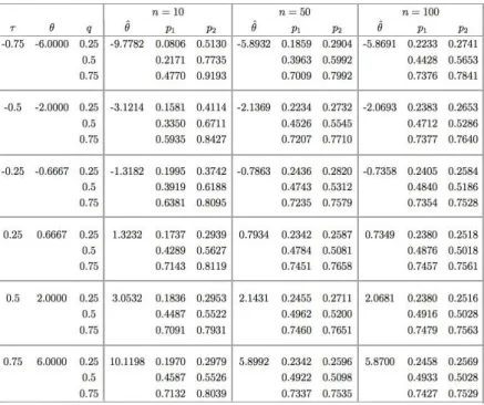
1 (13)The data were simulated from a copula family and parametric method copula were used in this simulation study;
Table 1. Simulated data from Clayton with estimated density copula,θˆ..
Based on the performance in table 1, we can see that all the values q∈[p1, p2]. 3.2 Example: survival analysis data
These data describe the lengths of time required for patients with headaches to achieve relief, each patient receives a standard treatment and a new treatment on separate occasions. The times are recorded to the nearest tenth of a minute [1]. Let (X, Y) denote the bivariate variable (the time to relapse of theithpatient on the first treatment, the time to relapse
of theithpatient on the second treatment), and suppose that we are interested in the ratio of
these two values for the next observation, Dn+1 = Yn+1/Xn+1 > d where, without loss of
generality,X >0.
For these data, we used bivariate Normal copula, C (θˆ) and the lower and upper probabilities for the event are presented in fig.1.
1inf
q dd
S
q
S d
q
(11)The proposed method performs well, if the two following inequalities hold,
1 1 1 N j j f q j p d d q N
1 (12)
2 1 1 N j j f q j p d d q N
1 (13)The data were simulated from a copula family and parametric method copula were used in this simulation study;
Table 1.Simulated data from Clayton with estimated density copula,θˆ..
Based on the performance in table 1, we can see that all the values q∈[p1, p2]. 3.2 Example: survival analysis data
These data describe the lengths of time required for patients with headaches to achieve relief, each patient receives a standard treatment and a new treatment on separate occasions. The times are recorded to the nearest tenth of a minute [1]. Let (X, Y) denote the bivariate variable (the time to relapse of theithpatient on the first treatment, the time to relapse
of theithpatient on the second treatment), and suppose that we are interested in the ratio of
these two values for the next observation, Dn+1 = Yn+1/Xn+1 > d where, without loss of
generality,X > 0.
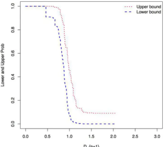
For these data, we used bivariate Normal copula, C (θˆ) and the lower and upper probabilities for the event are presented in fig.1.
Fig. 1.Upper and Lower ProbabilitiesDn+1.
4 Conclusion
Generally, the main conclusion we draw from the prediction performance of this method is performed well for small values of n, while for larger data sets a nonparametric copula can be used in order to learn more about the dependence structure from the data. The imprecision of the proposed method provides a sufficient robustness which consider to have a good frequentist properties specifically for the predictive inferences. The results is depending on the parametric copulas used, the random quantity and the percentiles studied. The imprecision decreases for increasing sample size
.
Acknowledgments
The author gratefully acknowledged the financial support received in the form of university research grant from Universiti Malaysia Pahang (RDU 170359).
References
1. Gross A J and Lam C F 1981Biometrics505–511
2. Melo L, Schneider R, Manso R, Saucier J P and Fortin M 2017 Canadian Journal of Forest Research
3. Wang X, Wang X, Hodgson L, George S L, Sargent D J, Foster N R, Ganti A K, Stinchcombe T E, Crawford J, Kratzke Ret al.2017The Oncologisttheoncologist–2016 4. Roy D 2017 Univariate and Multivariate Survival Models with Flexible Hazard
FunctionsPh.D. thesis
5. Cook T, Zhang Z and Sun J 2017Monte-Carlo Simulation-Based Statistical Modeling
(Springer) pp 319–346 [6] Chen L, Feng Y and Sun J 2017Lifetime data analysis23 651–670
6. Vodnala D, Sharma A, Dean E, Kennedy K, Magalski A and Austin B 2017Journal of
Cardiac Failure23S117
7. Risselada M, van Bree H, Kramer M, Chiers K, Duchateau L, Verleyen P and Saunders J H 2006 American Journal of Alzheimer’s Disease and Other Dementiasournal of
8. Coolen F P A 2011 International Encyclopedia of Statistical Science ed Lovric M (Springer) pp 968–970
9. Muhammad N 2016 Predictive inference with copulas for bivariate data Ph.D. thesis Durham University
10. Coolen-Maturi T, Coolen F P and Muhammad N 2016Journal of Statistical Theory and
Practice10515–538
11. Sklar A W 1959 Publications de lSInstitut de Statistique de lSUniversit´e de Paris 8 229–231
12. Joe H 1997 Multivariate models and multivariate dependence concepts vol73 (CRC Press)