Leakage detection in water pipe networks using a Bayesian probabilistic framework

(1)

Leakage detection in water pipe networks using

a Bayesian probabilistic framework

Z. Poulakis, D. Valougeorgis, C. Papadimitriou*

Department of Mechanical and Industrial Engineering, University of Thessaly, Pedion Areos, Volos 38334, Greece Received 17 November 2002; revised 1 July 2003; accepted 1 July 2003

Abstract

A Bayesian system identification methodology is proposed for leakage detection in water pipe networks. The methodology properly handles the unavoidable uncertainties in measurement and modeling errors. Based on information from flow test data, it provides estimates of the most probable leakage events (magnitude and location of leakage) and the uncertainties in such estimates. The effectiveness of the proposed framework is illustrated by applying the leakage detection approach to a specific water pipe network. Several important issues are addressed, including the role of modeling error, measurement noise, leakage severity and sensor configuration (location and type of sensors) on the reliability of the leakage detection methodology. The present algorithm may be incorporated into an integrated maintenance network strategy plan based on computer-aided decision-making tools.

Keywords:System identification; Bayesian method; Leakage detection; Water pipe networks

1. Introduction

Pipe networks represent one of the largest infrastructure assets of industrial society. In many cases these networks suffer from aging and deterioration and fail to fulfill the specified carrying capacities and required pressure heads. The high maintenance and revamping costs, including rehabilitation, replacement and/or expansion of existing systems to meet current and future demands give rise to difficult decision-making. All these activities, due to the large amount of money to be invested, usually become of primary public interest.

One of the major problems to be faced is the frequent pipe-breaks with unaccounted water leakages resulting in service disruption. Water service companies have begun to develop new leakage detection strategies in order to reduce

leakages to an economical optimum level [1]. The main

objective is to propose reliable computational models to facilitate pipe replacement decisions in an effort to increase the overall reliability expected from the pipe network.

An extensive amount of work on pipe rehabilitation and replacement has been published. The various algorithms

developed have taken the form of non-linear, dynamic, heuristic and successive linear programming economic models, which assist decision-making based usually on historical statistics and cost information. In an early work

Shamir and Howard[2]proposed a model, which estimates

the optimal time for pipe replacement based on pipe breakage history and the cost for repairing and replacing

pipes. Kettler and Goulter [3], identified a relationship

between breakage rate and pipe diameter as well as a correlation between the number of pipe failures and pipe age. They proposed that improvements to pipe breakage or mechanical reliability may be achieved by selecting larger

pipe diameters. Woodburn et al. [4]presented a model for

determining the minimum cost for rehabilitation, replace-ment or expansion of an existing network based on a combination of non-linear optimization and hydraulic simulation procedures. An explicit algorithm, implementing a graph theory approach, has been developed by Boulos and

Altman [5]. The algorithm is capable of handling

wide-spread applications, associated with future planning, expansion and improvement of fluid distribution networks. Arulraj and Rao[6]proposed an optimality criterion called the significance index to rehabilitate existing networks.

doi:10.1016/S0266-8920(03)00045-6

www.elsevier.com/locate/probengmech

* Corresponding author. Tel.: þ30-24210-74006; fax: þ 30-24210-74012.

(2)

since pipes are coming in discrete lengths and diameters.

Kim and Mays [7] resolved the problem, to some extent,

using integer pipe lengths as decision variables. More recently an increasing number of researchers are imple-menting genetic algorithm techniques in certain aspects of the design and rehabilitation of pipe networks, e.g. Murphy

et al. [8] and Simpson et al. [9]. Over the years genetic

algorithms have proven to be a reliable technique for handling water distribution network problems. In addition to their ability to handle discrete pipe diameters they have been shown to be quite robust and efficient in searching for optimal rehabilitation policies[10,11]. Following all these efforts water distribution companies have started lately, very reluctantly however, to implement these computational approaches and corresponding software as decision-making tools in the management of their water networks[1].

An issue, which is clearly related to an efficient leakage reduction policy but which has received much less attention, is the on-line leakage identification. Most of the research works performed and discussed above are not focused on leakage detection. It is mostly related to the general issue of developing efficient algorithms leading to optimal replace-ment, rehabilitation or expansion solutions for pipe net-works. Real-time damage estimation and diagnosis of buried pipelines, however, plays an important role in an integrated maintenance network strategy. Leakage detection may be considered, of course, as part of a typical calibration procedure and can be handled via optimization algorithms using conventional and evolutionary approaches. It is important, however, that the proposed algorithm is capable of incorporating in a quantitative manner all the errors in the model compared to the real problem. As reported by Goulter

and Bouchart [12], very little research work has been

reported on the inclusion of these probabilistic issues in optimization design models for water distribution networks. It is helpful to have a methodology to convert all these uncertainties and errors introduced in water pipe network optimization modeling into a measurement of the reliability of the results obtained by the modeling procedure. Here we address this issue focusing on leakage identification algorithms.

Leakage can be detected by correlating changes in flow characteristics to changes in a hydraulic model for the network. Significant changes in the hydraulic model are indicative of the location and the severity of the damage. This correlation is achieved by updating the hydraulic model so that its predictions match the measured data obtained from the sensors. This model updating procedure is an inverse problem that is usually ill-conditioned due to lack of sensitivity of the flow characteristics to modest amounts of leakages, and often non-unique due to insufficient available data relative to the model (network) complexity. Difficulties associated with the development of effective model updating and leakage detection algorithms are: (1) modeling errors (difference between theoretical model and actual system behavior), (2) measurement errors, and

(3) incomplete set of observed data due to limited number of sensors available or due to limited accessibility within the network.

Very recently Shinozuka and Liang [13] developed an

approach to identify the location and the severity of damage in a water delivery system by monitoring on-line water pressures at some selected positions of the network. Their damage detection approach is based on a neural network

inverse analysis method. Also Andersen and Powell [14]

proposed a leak detection scheme based on an implicit formulation of the standard weighted-least-squares state-estimation problem. In both cases however, the schemes are applied to idealized noise-free conditions.

In the present work a Bayesian system identification methodology is proposed for model updating which allows for the explicit treatment of the uncertainties arising from modeling errors and measurement noise. The methodology has been well developed and successfully applied in structural model updating applications [15 – 18]. Here, the Bayesian methodology is modified accordingly and it is coupled with hydraulic simulations for updating a para-meterized class of hydraulic models with the parameters chosen to simulate a set of possible leakage events (location and severity of leakage) in the pipe network. The methodology provides estimates of the probability of each leakage event (leakage location and severity) given the flow and/or pressure head measurements obtained from an integrated monitoring and data management system set up for the network. The most probable leakage event is identified as the one with the highest probability, while the other leakage events are ordered according to their relative probabilities. The effectiveness of the proposed framework is illustrated by applying the leakage detection approach to a specific water pipe network. Several important issues are addressed, including the role of modeling error, measurement noise and sensor configur-ation (locconfigur-ation, number and type of sensors) on the reliability of the leakage detection methodology.

2. Formulation

A typical hydraulic formulation is used for the solution of the water pipe network. The flow equations to be solved consist of the mass conservation equations at the junction nodes and the energy conservation equations around the loops and the pseudo-loops of the network[19]. The system is solved using a Newton iteration scheme. Once the pipe flow rates are estimated the energy grade at the nodes is explicitly estimated through a marching procedure.

Leakage detection is based on the premise that damage (leakage) in one or more locations of the piping network involves local liquid outflow at the leakage location, which will change the flow characteristics (pressure heads, flow rates, acoustics signals, etc.) at the monitoring locations of the piping network. The magnitude of

(3)

changes in the flow characteristics depends on the position and the severity of the damage (amount of outflow). The existence of leakage in the pipe network is diagnosed by monitoring the permanent changes in the flow character-istics of the system. Once the existence of the damage has been diagnosed, it is possible by updating the hydraulic model for a complete set of parameters to identify the location and the severity of the damage. For this, a statistical system identification methodology is applied that effectively tackles the uncertainties due to modeling error and measurement noise.

2.1. Statistical system identification

The hydraulic pipe network formulation is implemented to generate a class of solutions describing the flow behavior of the piping distribution system in an undamaged state or in a damaged (deteriorated) state due to leakage events. This class of solutions is generated from a parameterized class of models denoted byM:Letube the parameters introduced in the parameterized class of hydraulic modelsM:In the case of leakage identification these parameters are associated with the location and extend of the damage in the piping distribution system. A particular modelMðuÞfrom the class Mis selected by specifying the values of the parameter setu:

Next consider a monitoring system that has been installed in the network in order to collect and analyze data obtained fromNflow tests performed periodically atL monitoring locations. Let~xijbe the available flow data from thejth flow testð1#j#NÞobtained at theith monitoring

location ð1#i#LÞ_: Without loss of generality we may

assume that the flow data set may consist of pressure heads

~

Pand flow rates Q~ estimates obtained at theL monitoring locations. Letx~¼ ½x~ijdenote theL£Nmatrix of data atL locations fromN flow tests.

Let alsoxðuÞ ¼ ½xijðuÞ be the flow quantities (pressure heads, flow rates, etc.) at the monitoring locations computed

from the model MðuÞ corresponding to a particular value

assigned in the parameter setu:The departure between the model results and the corresponding measured flow quantities, defined by

eijðuÞ ¼~xij2xijðuÞ ð1Þ

measures the prediction error from the modelMðuÞ: This departure is due to flow network modeling error and device measurement accuracy that are unavoidable in the modeling process of real water distribution systems.

System identification is handled by employing a statistical approach[15,20] in which the model prediction error eijðuÞ is considered to be a specific realization of a random variable taken from a class of probabilistic error modelsP;parameterized by the parameter sets:The class

of pipe flow models M and the class of prediction error

modelsP;which specify the modeling assumptions used in

the description of the system, are parameterized by the parameter set½u;s:

The objective of the statistical system identification methodology is to update the values of the parameter set ½u;sand their associated uncertainties using the measured test data. Here, uncertainty in the values of the parameter set is quantified using probability density functions (PDF), which measure the relative plausibility of each of the

models in classes M and P specified by the parameters

½u;s:The selection of the parameter uncertainty prior to the collection of data is based on engineering experience and it is quantified by the initial PDF pðu;sÞ: Using Bayes theorem, this initial PDF is converted to a posterior (updated) PDF

pðu;slxÞ ¼~ c₁pð~xlu;sÞpðu;sÞ ð2Þ

which gives the relative plausibility of the models based on the inclusion of the measured data x~:The constantc₁ is a normalizing constant selected such that the posterior PDF pðu;slxÞ_~ is integrated to one. In Eq. (2) the expression for

the posterior PDFpðu;slxÞ~ depends on the chosen classes of

pipe network modelsM;the prediction error modelsPand

the measured data.

Assuming eijðuÞ; i¼1;…;L; j¼1;…;N to be inde-pendent and normally distributed with zero mean and standard deviation s; the likelihood pðx~lu;sÞ may be

written in the form pðx~lu;sÞ ¼Y L i¼1 YN j¼1 1 ffiffiffiffi 2p p sexp 2 ðxijðuÞ2~xijÞ2 2s2 " # : ð3Þ Assuming also a non-informative prior distribution for the model parameters over the range of acceptable values of ½u;s; i.e. assuming that the initial PDF pðu;sÞ is constant, and substituting Eq. (3) into Eq. (2) yields

pðu;slxÞ ¼~ c₂ 1 ðpffiffiffiffi2psÞLNexp 2 XN j¼1 kx_jðuÞ2x~_jk2 2s2 2 6 6 6 6 6 4 3 7 7 7 7 7 5 ð4Þ

where k·k is the usual Euclidean norm. The vector x_jðuÞ

denotes the model results, while the vector x~j denotes the corresponding measured flow quantities at the measured locations from thejth flow test. The constantc2 in Eq. (4) is selected such that the posterior PDF pðu;slxÞ~ is

integrated to one.

2.2. Optimal model and model uncertainty

The optimal value of the model parameters denoted by ½_u^_;_s_^_;_{is simply the most probable value of}_½_u_;_s_obtained

by maximizing the updated PDFpðu;slxÞ_~ _{or equivalently by}

minimizing the function gðu;sÞ ¼2ln½pðu;slxÞ~ ¼ 1 2s2 XN i¼1 k~x_i2x_iðuÞk2þ LN 2 lns 2_þ_c_: _ð5Þ

(4)

The optimal½_u^_;_s_^_{for a given sensor configuration depends}

only on the datax~:Performing the optimization for a set of continuous parameters u; it can be readily shown that the

optimal values u^ of the network model minimize the

function JðuÞ ¼ 1 LN XN j¼1 kx_jðuÞ2x~_jk2 ð6Þ

whereJðuÞrepresents a norm of the difference between the model and the measured output. Through the optimization procedure it can also be shown that the optimal values^2of the prediction error model is

^

s2¼Jðu^Þ: ð7Þ

In particular, using the total probability theorem, the marginal probability distribution foruis obtained as pðulxÞ ¼~

ð

pðu;slxÞd~ s: ð8Þ

Substituting Eq. (4) into Eq. (8) and after some mathemat-ical manipulation, using Eq. (6) and assuming a uniform initial distribution pðu;sÞ the integration in Eq. (8) is carried out analytically to yield

pðulxÞ ¼~ c½JðuÞ2ðLN21Þ=2: ð9Þ

For a general initial distribution pðu;sÞ an asymptotic approximation is available in the form[21]

pðulxÞ ¼_~ c½JðuÞ2ðLN21Þ=2gðuÞ ð10Þ

wheregðuÞ ¼pðu;pffiffiffiffiffiJðuÞÞ:Expression (9) or (10) yields the uncertainty in the optimal estimate of the model parameters given the measured data.

2.3. Application to leakage detection

Consider the case of network deterioration due to the presence of fractures in one or more locations of a water pipe network consisting ofppipes. Such events will involve local water outflows that can be modelled by adding a flow demand at each fractured pipe indicating the location of each leakage. In addition the amount of each flow demand will correspond to the severity of the leakage in that location.

LetKbe the number of leakage locations. The amount of

flow demands and the leakage locations (pipe locations where these demands are added) constitute the set of

unknown parametersuof the integrated class of modelsM

describing the behaviour of the system with leakages. The following model parameterisation can be adopted to efficiently identify the leakage in the network assuming that leakage occurs atKlocations. The model parameter set

uis partitioned into two subsets written asu¼ ðul;usÞ:The subsetulis aK-dimensional vector of integers denoting the pipe sections that have leakage, i.e. denoting the locations of leakage in the network. The total number of distinct leakage

events in a water distribution system with p pipe sections andKleakage locations is

NK ¼ p!

K!ðp2KÞ!: ð11Þ

The subset us is also a K-dimensional vector giving the

amount of liquid outflow, quantifying the leak severity

(amount of leakage) at the corresponding K leakage

locations identified in the setul: The optimal valuesu^¼ ð_u^

l;u^sÞof the model parameters

u¼ ðul;usÞ are computed by maximizing expression (9). This optimization problem involves a mixed set of discrete and continuous variables. The discrete variables, included in the parameter subset ul; take integer values from 1 to p; indicating the number of the pipe that has leaked, while the continuous variables, included in the parameter subset us; can only take positive values since leakage involves liquid outflow.

The solution scheme that is adopted to solve the

optimisation problem withK leakages involves an

exhaus-tive search over the discrete parameter subspace. Specifi-cally, letuðliÞdenote the leakage locations corresponding to the ith leakage event taken from the total of NK distinct

leakage events. The most probable value u^ðiÞ

s of the

parameter set us; given that leakage occurs at locations

uð_liÞ; are obtained by maximizing the PDF, given by

expression (9), with respect to the parameters in the setus:

This is a continuous optimisation problem involving theK

parameters in the set us: Then the most probable leakage event u^l is the one of u

ð1Þ l ;u

ð2Þ l ;…;u

ðKÞ

l that maximizes the

updated PDF function pðuð_liÞ;u^sðiÞl~xÞ ¼c½Jðu ðiÞ l ;u^ ðiÞ s Þ 2ðLN21Þ=2_: ð12Þ

Thus the most probable leakage event u^¼ ð_u^

l;u^sÞ can be obtained by solving a series ofNKoptimization problems.

An exhaustive search of the most probable leakage event

requires the solution of NK optimization problems which

may be computationally expensive or even prohibitive, considering that each function evaluation ofxðuÞinvolved in Eq. (9) requires the solution of a non-linear algebraic system of equations governing the steady-state flow in pipe

networks. Instead, genetic algorithms [22] can be used to

efficiently solve this type of discrete optimization problem in order to provide a near optimal solution for the leakage locations.

In practice, it is expected that deterioration will proceed progressively with leakage occurring at one location at a time. Using a monitoring system, the algorithm could be used to search for single leakages. This involves the solution

of as many asNK ¼poptimization problems and thus the

computational effort is relatively small. Furthermore, when the leakage locations are expected to occur only in a certain number of pipes forming the network the computational complexity of the problem is significantly reduced, even for the case of searching for multiple leakage locations.

(5)

To conclude the theoretical formulation of the method-ology, it is stated that the leakage detection in networks with multiple leaking events involves a continuous optimization problem searching for the leakage severity, which is embedded in a discrete optimization problem searching for the most probable leakage location.

3. Application to networks

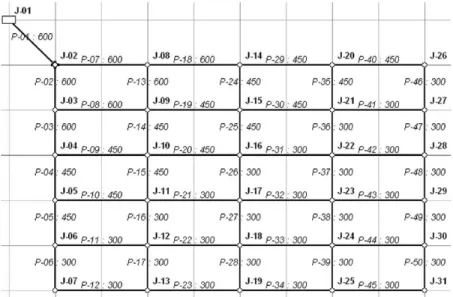
In order to demonstrate the effectiveness and efficiency of the proposed leakage detection method-ology the whole approach is applied to an example

network shown in Fig. 1. This network can be

considered as a simplified, typical, municipal water distribution system or a water distribution network for an industrial unit. It comprises 50 pipe sections, 31 junction nodes and 20 loops (no pseudo-loops). The water is supplied from an elevated tank by gravity. The lengths of the horizontal and vertical pipe sections are 1000 and 2000 m, respectively, and the elevation of the tank is 52 m. Pipe and junction numbering is given in Fig. 1, where the pipe diameters, varying from 300 to 600 mm, are also indicated. Flow demands are assumed at each node of the network throughout the water delivery system. The water flow is in the turbulent flow regime with a friction factor estimated by the formula of

Swamee and Jain [19].

The class of models used for identifying leakage in the network assumes that the piping-roughness coefficients are the same for all pipes and the flow demands are uniform throughout the water delivery system. The nominal values for the piping-roughness coefficients are taken to be equal to 0.26 mm for all pipes and the flow demands are assumed equal to 50 l/s at each junction node. The total volume of water supplied from the elevated tank is 1550 l/s and is equal to the total flow demands in the network.

3.1. Data simulation

Measured data are simulated from a pipe network model with characteristics that are different from the ones that correspond to the class of models used for monitoring and identification of the network condition. The measured data produced in this way allows the simulation and study of the model error effect on the leakage detection results. In addition, in order to account for the measurement noise in the sensors, an error term is added to the predictions of the perturbed model to simulate the observed discrepancy between the actual pipe network predictions and the measurements from the sensors.

Specifically, the simulated measured data are generated from the following equation

~ xij¼~x m ij þx~ n ij; 1#i#L; 1#j#N: ð13Þ

The first term,x~mij;in Eq. (13) represents the pressures and/or the flow rates that are generated from a class of pipe network models with characteristics that deviate from the nominal characteristics defining the class of models used for identification. Here, the characteristics that are perturbed from their nominal values include the piping roughness coefficients in each pipe and the flow demands at the nodes. The perturbation from the nominal values of the piping-roughness coefficients for each pipe and of the flow demands for each node is assumed to follow a zero-mean uniform distribution with bounds ð2a;aÞ and ð2b;bÞ; respectively. The size of the perturbation, that is, the values

of a and b; represents the magnitude of the model error

expressed as a percentage of the nominal values of the system characteristics. The statistical generation of these perturbations reflects the uncertainty in the actual values of these parameters. Hereafter, the aforementioned perturbed model is assumed to be representative of the actual behaviour of the system and is referred to as the ‘actual system’.

(6)

It is obvious that when the above procedure to simulate the measured data is used, the class of models for identification is not capable of representing the behaviour of the actual system exactly. Following this approach it is possible to simulate and study the effects of the model error on the leakage detection results.

The second term, ~xnij; in Eq. (13) accounts for the measurement error that comes from the sensors. It is chosen to be a zero-mean, uniformly distributed random variable with boundsð2c;cÞ:The magnitude ofcrepresents the size of measurement error at a measured location expressed as a percentage of the actual system predictions at the measured location.

Depending on the type of the measured data used in the identification procedure, two cases, namely Cases A and B, are considered separately. In Case A the measured data consists of pressures at junction nodes, while in Case B the measured data consists of flow rates in pipes. For demonstration purposes, the case of a single leakage and the case of two leakages are examined separately.

3.2. Detection of a single leakage

The case of a single leakage ðL¼1Þ located at pipe

section 26 is considered. Seven monitoring devices are used, spread all over the network and relatively far from the vicinity of the leaked pipe 26. For Case A the manometers are located at the junction nodes 6, 9, 13, 18, 21, 25 and 30, while for Case B the flow meters are located at the pipe sections 1, 3, 16, 19, 29, 36 and 43. The leakage location is simulated by adding a node at the damaged pipe while the prescribed flow demand corresponds to the amount of leakage at the leakage location. Simulated measured data are generated from Eq. (13) using the actual system with the corresponding leakage location.

The problem of identifying the leakage location and severity is addressed given that only a single leakage is

expected. The number of possible leakage scenarios, given in Eq. (11), is equal to the number of pipe sections in the

water network ðNK¼50Þ: The class of models used for

leakage identification involves two parametersðul;usÞ;with

ul denoting the leakage location andus accounting for the amount of leakage.

By means of the identification procedure, first the most probable amounts of leakageu^ðsiÞof the parameter setuðsiÞare estimated for each leakage scenario i: In the case of the single leakage,iindicates the pipe number that has leaked. Then the normalized probability

pi¼kpðu ðiÞ l ;u^

ðiÞ

s lxÞ~ ð14Þ

of each leakage eventiis computed, for the corresponding most probable leakage severity value u^ðiÞ

s :The values ofpi establish an order for the leakage events according to their relative normalized probability. The most probable leakage event is identified as the one with the highest

normalized probability pi: The normalizing constant,

k¼PNK i¼1pðu

ðiÞ l ;u^

ðiÞ

s lxÞ~ ; is conveniently used for plotting purposes without affecting the interpretation of the results. 3.2.1. Idealized scenario with no errors

First, no model or measurement uncertainties are

introduced ða¼b¼c¼0%Þ: The amount of leakage is

taken to be equal to 22.8 l/s, which corresponds to 1.5% of the total water volume supplied in the network. The

computed peak values of the normalized posterior PDF pi

are plotted in Fig. 2A and Bfor each pipe section of the

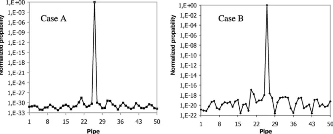
water distribution network for Cases A and B, respectively. It is seen that in both cases tested, although the leakage severity is quite small compared to the total water volume, the proposed methodology identifies correctly the pipe where the leakage is assumed. When no model or measurement uncertainties are introduced, the peak value of the posterior PDF of the most probable scenario is equal to one, while the corresponding values for all other

Fig. 2. Peak values of normalized PDF at each pipe section using (A) manometers and (B) flow meters. Leakage is located at pipe 26 with severity equal to 22.8 l/s (1.5% of the total water volume).

(7)

undamaged pipes are identically equal to zero (within round-off error), independently of the leakage severity. This is a typical result for all cases tested, and in this way the assumed location and severity of the leakage is easily found. 3.2.2. Effect of model errors

The above situation is highly idealized and almost never occurs in real water delivery systems. More realistic situations are simulated next, when some model errors are introduced by imposing perturbations in the values of the roughness coefficient and the flow demands. The amount of leakage is taken to be equal to 22.8 l/s.

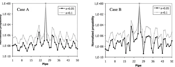
First, perturbations equal to 5 and 10% are introduced

in the model error magnitude a; corresponding to the

piping roughness coefficient. The results related to the identification of the leakage location are plotted inFig. 3A and Busing manometers (Case A) and flow meters (Case B), respectively. The most probable leakage scenario predicts leakage in pipe 26, which coincides with the actual leakage location. Again, the peak values of the posterior PDF of the most probable leakage event are several orders of magnitudes larger than the correspond-ing values of the other leakage scenarios. This is an indication that the location of the damaged pipe is clearly identified even for small amounts of leakage compared to the nominal flow rate of the particular pipe and for relatively large model error introduced in the parameter-ized model.

The computed amounts of leakage are compared to the

actual amounts inTable 1for Cases A (Figs. 2A and 3A)

and B (Figs. 2B and 3B). It is seen that whena¼0% the

actual amounts of leakage are exactly estimated. Fora¼5 and 10% there is some departure between the computed and the actual amounts when the experimental data are obtained using pressure-measuring devices. The higher the model error is, the higher is the departure between the identified and the actual amounts of leakage. The agreement is excellent when flow meters are used.

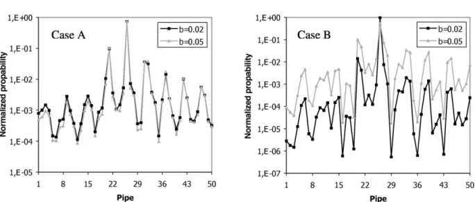
We continue our study on the effects of the model uncertainties on the leakage identification process by implementing a second mechanism to introduce model errors. The nominal values of the flow demands are

perturbed by an amountbequal to 2 and 5%.Fig. 4A and B

shows the corresponding normalized peak values of the posterior PDF in each pipe for Cases A (manometers) and B (flow meters), respectively. It is seen that the departure of the peak values of the posterior PDFs between the most probable scenario and the second most probable scenario becomes smaller compared to corresponding previous results (Fig. 3A and B). It is pointed out however, that the most probable leakage scenario coincides with the actual leakage event. Even for a small leakage equal to 1.5% of the total water supply and for an uncertainty equal to 5%, the departure between the most and the second most probable events is at least one order of magnitude. It is worth noting that the second most probable leakage scenario corresponds to leakage at pipe 21, which is adjacent to pipe 26.

It should be noted, however, that for even more difficult situations involving even smaller amounts of leakage and/or larger uncertainties (larger model errors) it will not be possible to identify successfully the leakage location. There is always a threshold level beyond which no reliable results are obtained. The proposed methodology is capable of identifying these threshold values. In many cases when the accurate leakage location is not possible it is still useful to Fig. 3. Peak values of normalized PDF at each pipe section using (A) manometers and (B) flow meters. Leakage is located at pipe 26 with severity equal to 22.8 l/s (1.5% of the total water volume). A perturbationa¼5 and 10% is assumed in the piping roughness coefficient.

Table 1

Comparison between computed and actual amounts of leakage in pipe 26 for various uncertainties in the pipe roughness coefficient using (A) manometers and (B) flow meters

Case Actual leakage (l/s) Computed leakage (l/s)

a¼0 a¼5% a¼10%

A 22.8 22.8 26.9 30.4

(8)

identify the region in the pipe network which contains the damaged pipe.

InTable 2the computed amounts of leakage for Cases A (Figs. 2A and 4A) and B (Figs. 2B and 4B) are compared to the actual amounts. It is seen that the leakage severity for

b¼0 is computed exactly, while for b–0 it is

over-estimated. It is evident that for the water pipe network under investigation the estimation of leakage severity is particu-larly sensitive to demand variations. In these cases, an improved sensor placement configuration capable of collecting better information from the network is essential and will resolve to some extend the problem. It is seen that, for the pipe network under examination, the identification of the amount of leakage is less accurate than the correct identification of the leakage location when uncertainties in the demands are introduced—in the sense that this identification is more sensitive to model errors.

In general, as expected, the departure between computed and actual quantities becomes larger as the leakage severity is decreased and as the model errors are increased. 3.2.3. Effect of measurement errors

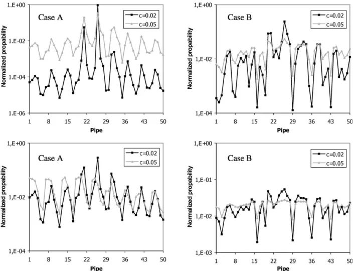
The study on the effects of the errors is completed by implementing additional uncertainties due to measurement errors. These errors are again simulated by adding a zero-mean uniform noise in the data generated by the actual

system, with a standard deviation cequal to 2 and 5% of

the actual system predictions at the measured locations. Two leakage severity scenarios are considered which correspond to leakage amounts equal to 57.0 and 22.8 l/s, which represent 3.7 and 1.5%, respectively, of the total

supplied water volume (1550 l/s). In Fig. 5A and B the

computed peak values of the posterior PDF are plotted for each leakage scenario and for each pipe section of the water distribution network for Cases A and B, respectively. For c¼2% the leakage location is correctly identified for all cases. It is worth noting that the second most probable

leakage location predicted by the methodology is pipe 20 or 21, which is very close to the correct leakage location. For larger measurement errorsðc¼5%Þthe leakage location is correctly identified for the cases of 57.0 l/s. However, for the smaller leakage of 22.8 l/s, the correct leakage location is not identified in Case A. It is interesting to note that this small amount of leakage corresponds to 1.5% of the total water supply. Moreover, in Case B, although the correct leakage location is identified as the most probable, other leakage locations have been predicted with a probability close to that. In addition, inTable 3the computed amounts of leakage for Cases A (Figs. 2 and 5) and B (Figs. 2B and 5B) are compared to the actual amounts. Forc¼0;the correct amount of leakage is clearly identified and the exact amount of leakage is computed. It is also noted that for

c–0 the amounts of leakage, as is shown inTable 3, are

computed with good accuracy for all cases tested. It may be concluded that for the water pipe network under investi-gation the errors in the experimental data have a more serious effect on the sensitivity of the results related to the location rather than the severity of the leakage.

3.2.4. Effect of sensor type and location

We conclude this section by investigating the effect of the positioning of the measuring devices on the system identification methodology. This is demonstrated by study-ing the same test case network shown inFig. 1. The leakage Fig. 4. Peak values of normalized PDF at each pipe section using (A) manometers and (B) flow meters. Leakage is located at pipe 26 with severity equal to 22.8 l/s (1.5% of the total water volume). A perturbationb¼2 and 5% is assumed in the demands.

Table 2

Comparison between computed and actual amounts of leakage in pipe 26 for various uncertainties in the demands using (A) manometers and (B) flow meters

b¼0 b¼2% b¼5%

A 22.8 22.8 38.7 61.5

(9)

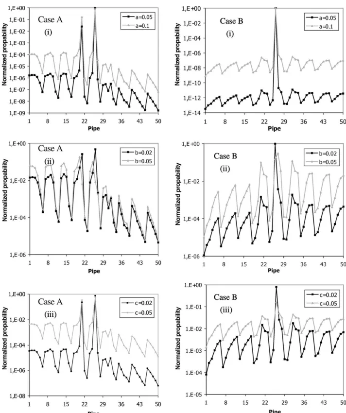
is kept in pipe 26 and only the case of leakage severity equal to 57.0 l/s, i.e. 3.7% of the total water supply is studied. The seven measuring devices, however, are placed in different positions. This new positioning, which can be either less or more informative about the system is such that the sensors are concentrated in certain sub-regions of the network. The manometers (Case A) are all located in the lower right region of the network, specifically at junctions 17, 18, 19, 23, 24, 25 and 31. The flow meters (Case B) are located in the upper left region of the network, specifically at the pipe sections 1, 2, 3, 7, 18, 25 and 26. The flow meter configuration includes a sensor, which is located at the leaking pipe 26.

InFig. 6A and Bthe computed normalized peak values of the posterior PDF are plotted for each pipe section of the water distribution network using manometers (Case A) and flow meters (Case B), respectively. All three different types of uncertainties involving the pipe roughness coefficientsa;

the flow demands b and the measurement data c are

examined. Consequently, a direct comparison between the present results and those obtained with the previous measuring devices configuration is possible. Comparison

of the results inFigs. 3 and 6(i)dealing with uncertainties in pipe-roughness coefficients shows that with the new sensor configuration the identification results are improved for the case of flow measurements, while they have deteriorated for the case of pressure measurements. Comparison of the results inFigs. 4 and 6(ii)dealing with uncertainties in flow demands shows that the identification results obtained from the new sensor configuration are less informative for both the cases of flow and pressure measurements. In particular, Fig. 5. Peak values of normalized PDF at each pipe section using (A) manometers and (B) flow meters. Leakage is located at pipe 26 with severity equal to (i) 57.0 and (ii) 22.8 l/s (3.7 and 1.5% of the total water volume). A perturbationc¼2 and 5% is assumed in the modeled measurements.

Table 3

Comparison between computed and actual amounts of leakage in pipe 26 for various uncertainties in the measurement data and two different amounts of leakage using (A) manometers and (B) flow meters

c¼0 c¼2% c¼5%

A 22.8 22.8 23 23.3

57.0 57.0 57.0 57.0

B 22.8 22.8 24.3 25.3

(10)

the methodology fails to predict the actual leakage location for the case ofb¼5%:The most probable leakage location predicted by pressure measurements is in pipe 20 and in pipe 27 for flow rate measurements, both of which are adjacent to the damaged pipe 26. Finally comparison of the results in

Figs. 5(i) and 6(iii) dealing with uncertainties in the measured data shows that the identification results obtained from the new sensor configuration are significantly improved for both cases of pressure and flow rate measurements. Specifically, in contrast to the previous Fig. 6. Peak values of normalized PDF at each pipe section using (A) manometers in the nodes (17, 18, 19, 23, 24, 25, 31) and (B) flow meters in the pipe sections (1, 2, 3, 7, 18, 25, 26). Leakage is located in pipe 26 with severity equal to 57.0 l/s.

(11)

sensor configuration, which was not informative enough for accurate leakage predictions, the new sensor configuration provides reliable prediction of the position of leakage.

The above results indicate clearly that an optimal sensor placement strategy [23,24] is very important for efficient detection of damage in water pipe networks. The critical issue is to estimate the proper number and location of sensors in order to obtain the maximum possible infor-mation from the network without knowing in advance the location and amounts of leakage in the system. This is a difficult task which will be addressed in detail in later work. 3.3. Detection of multiple leakages

It has been shown in Section 2 that the proposed methodology is capable in a straightforward manner of studying simultaneous multiple leakages in a water distribution system. An application is presented in this

section using the water pipe network of Fig. 1, with two

leakages in pipe sections 26 and 42. The amounts of leakage are taken to be 114 and 44.7 l/s, which represent 7.4 and 2.9%, respectively, of the total water supply. It is noted that

while in the case of one leakage there are 50 possible leakage scenarios, now, with two leakages, it is estimated

using Eq. (11) with K¼2 and p¼50 that there are

Nk¼1225 possible leakage scenarios. It is obvious that the required computational effort is significantly increased. The implementation however of the whole approach remains the same.

The results from the identification methodology are very similar to the case of one leakage event. When no uncertainties exist in the system, the results indicate the two leakage locations and the corresponding amounts very accurately, independently of the positions and the amounts of leakage. When uncertainties are introduced, more careful investigation is required, since there are several leakage scenarios with a probability value close to the probability of the most probable leakage scenario.

Some typical results from the most probable leakage scenarios are presented in tabulated form. In Table 4, the first five most probable leakage events are given based on the use of manometers (Case A) and flow meters (Case B)

with introduced uncertaintya¼5% in the pipe roughness

coefficient. Each leakage event is described in terms of Table 4

The first five most probable leakage events with a perturbationa¼5% in the pipe roughness coefficient using (A) manometers and (B) flow meters. Actual leakage locations are in pipes 26 and 42 with corresponding amounts 114 and 44.7 l/s

Case Leakage location (pipe number) Leakage severity (l/s) Peak value of normalized PDF

Location 1 Location 2 Severity 1 Severity 2

A 26 42 113.4 44.0 1.000 26 43 118.2 30.1 1.494£1022 26 46 107.1 65.1 1.972£1025 26 47 112.9 47.6 1.775£1025 26 41 106.2 67.7 1.671£1025 B 26 42 114.2 44.7 1.000 26 48 109.4 49.6 7.778£1025 26 37 107.0 52.0 1.324£1025 26 36 121.3 37.5 6.857£1026 26 47 118.9 39.9 5.922£1026 Table 5

The first five most probable leakage events with a perturbationb¼2% in the demands using (A) manometers and (B) flow meters. Actual leakage locations are in pipes 26 and 42 with corresponding amounts 114 and 44.7 l/s

A 26 42 115.9 42.0 1.000 26 43 120.6 28.6 8.816£1022 26 41 109.0 64.8 3.902£1022 26 31 105.5 64.4 3.445£1022 26 46 109.9 62.2 2.849£1022 B 26 42 114.7 43.5 1.000 26 48 109.9 48.3 1.118£1022 26 37 107.5 50.7 1.279£1023 26 43 103.9 54.3 1.098£1024 26 47 119.3 38.8 6.140£1025

(12)

the two-leakage location and severity and its corresponding normalized probability. The probability results shown in the last column have been normalized such that for each case the most probable leakage event corresponds to probability equal to one. Similar results are given inTables 5 and 6for introduced uncertainties in the demandsðb¼2%Þand in the experimental dataðc¼2%Þ;respectively. It is seen that in most cases the ‘actual leakage event’ is estimated correctly. Again it has been found that as the amount of leakage is reduced and the model and measurement errors are increased there are certain threshold values of model and measurement errors above which the identification of the leakage event is not possible.

The results in Tables 4 – 6 have been obtained using a

combinatorial approach searching for all possible leakage scenarios. For more than two leakages, genetic algorithms

[22] may be implemented in order to sustain reasonable

computational effort and time levels converging to the near global solution.

4. Conclusions

A Bayesian probabilistic framework for leakage detec-tion in water pipe networks has been developed and successfully tested with simulated data. Prediction of the most probable leakage locations and severity involves a series of continuous optimization problems followed by a discrete optimization problem. For the cases considered, an exhaustive search is used to solve the discrete optimization problem. When the system is free from model error and measurement noise, the model is capable of identifying the damage ‘exactly’. More realistic circumstances are also examined in detail by introducing uncertainties in the hydraulic model and the measurement data.

The procedure is applied to a sample network for the case of a single and of multiple leakages and the effectiveness of the new methodology is demonstrated. The location of the leakage is correctly identified and its severity is accurately

computed, when the model and measurement errors do not exceed certain threshold values above which the diagnosis of the system is not possible. These threshold values depend on the configuration and the characteristics of the water distribution system under investigation and the location and severity of leakage as well as the number, location and type of sensors. More important, the present approach is capable of identifying these threshold values beyond which no reliable diagnosis is possible. The location of the measuring devices has a significant effect on the reliability of the system identification. Optimal sensor location strategies [23] can be used to improve the reliability of the leakage prediction estimates.

The present approach may be part of an integrated software to assist decision-making for overall water network management strategy based on computer-aided tools. The main principles of this work can be extended to compres-sible fluids.

Acknowledgements

This work has been partially supported by the Greek Secretariat of Research and Technology (PENED 1999-99ED580 and PAVET 2000-00BE72) and by the Athens Water and Sewerage Company. This support is gratefully acknowledged.

References

[1] Savic D, Walters G. Hydroinformatics technology and maintenance of UK water networks. J Qual Maintenance 1997;3(4):289 – 301. [2] Shamir U, Howard CD. An analytic approach to scheduling pipe

replacement. J Am Water Works Assoc 1979;71:248 – 58.

[3] Kettler AJ, Goulter IC. An analysis of pipe breakage in urban water distribution networks. Can J Civil Engng 1985;12(2):286 – 93. [4] Woodburn J, Lansey K, Mays LW. Model for the optimal

rehabilitation and replacement of water distribution system com-ponents. Proc Natl Conf Hydraul Engng, New York 1987;606– 11. Table 6

The first five most probable leakage events with a perturbationc¼2% in the measurement data using (A) manometers and (B) flow meters. Actual leakage locations are in pipes 26 and 4 with corresponding amounts 114 and 44.7 l/s

A 26 42 115.6 43.2 1.000 26 47 111.1 50.6 7.629£1021 26 43 118.0 31.3 2.310£1021 26 46 109.7 64.1 1.919£1021 26 40 100.5 85.1 5.236£1022 B 26 45 94.71 69.7 1.000 26 48 108.8 49.0 7.660£1021 26 34 97.54 53.9 7.213£1021 26 39 103.5 47.8 5.143£1021 26 38 98.74 60.2 3.469£1021

(13)

[5] Boulos P, Altman T. A graph-theoretic approach to exhibit nonlinear pipe network optimization. Appl Math Modeling 1991;15:459 – 66. [6] Arulraj P, Suresh RH. Concept of significance index for maintenance

and design of pipe networks. J Hydraul Engng 1995;121(11):833 – 7. [7] Kim HJ, Mays LW. Optimal rehabilitation model for water distribution systems. J Water Resour Plann Manage ASCE 1994; 120(5):674 – 92.

[8] Murphy LJ, Simpson AR, Dandy GC. Design of a network using genetic algorithms. Water 1993;20:40 – 2.

[9] Simpson AR, Dandy GC, Murphy LJ. Genetic algorithms compared to other techniques for pipe optimization. J Water Resour Plann Manage 1994;120(4):423 – 43.

[10] Dandy GC, Simpson AR, Murphy LJ. An improved genetic algorithm for pipe network optimization. Water Resour Res 1996;32(2):449 – 58. [11] Savic D, Walters G. Evolving sustainable water networks. Hydrol Sci

1998;42(4):549 – 63.

[12] Goulter IC, Bouchart F. Reliability-constrained pipe network model. J Hydraul Engng 1990;116(2):211 – 29.

[13] Shinozuka M, Liang J. On-line damage identification of water delivery systems. Engng Mech Conf 1999;.

[14] Andersen JH, Powell RS. Implicit state-estimation technique for water network monitoring. Urban Water 2000;2:123– 30.

[15] Beck JL, Katafygiotis LS. Updating models and their uncertainties— Bayesian statistical framework. J Engng Mech ASCE 1998;124(4): 455 – 61.

[16] Vanik MW. A Bayesian probabilistic approach to structural health monitoring. PhD thesis, California Institute of Technology, Pasadena, CA, 1997.

[17] Vanik MW, Beck JL, Au SK. Bayesian probabilistic approach to structural health monitoring. J Engng Mech ASCE 2000;126(7): 738 – 45.

[18] Katafygiotis LS, Lam HF. A probabilistic framework for structural health monitoring. Proceedings of the 12th Engineering Mechanics Conference, New York: ASCE; 1998. p. 1379 – 82.

[19] Potter MC, Wiggert DC. Mechanics of fluids. Englewood Cliffs, NJ: Prentice-Hall; 1997.

[20] Beck JL. Statistical system identification of structures. Proceedings of the Fifth International Conference on Structural Safety and Reliability, New York: ASCE; 1989. p. 1395 – 402.

[21] Katafygiotis LS, Papadimitriou C, Lam HF. A probabilistic approach to structural model updating. Int J Soil Dyn Earthquake Engng 1998; 17(7 – 8):495 – 507.

[22] Goldberg DE. Genetic algorithms in search, optimization and machine learning. Reading, MA: Addison-Wesley; 1999.

[23] Papadimitriou C, Beck JL, Au SK. Entropy-based optimal sensor location for structural model updating. J Vib Control 2000;6(5): 781 – 800.

[24] Udwadia FE. Methodology for optimal sensor locations for parameters identification in dynamic systems. J Engng Mech ASCE 1994;120(2):368 – 90.