Hittingtime and PageRank

SJSU ScholarWorks

Master's Theses Master's Theses and Graduate Research

Spring 2014

Hittingtime and PageRank

Shanthi Kannan

San Jose State University

Follow this and additional works at:https://scholarworks.sjsu.edu/etd_theses

This Thesis is brought to you for free and open access by the Master's Theses and Graduate Research at SJSU ScholarWorks. It has been accepted for inclusion in Master's Theses by an authorized administrator of SJSU ScholarWorks. For more information, please [email protected]. Recommended Citation

Kannan, Shanthi, "Hittingtime and PageRank" (2014).Master's Theses. 4424. DOI: https://doi.org/10.31979/etd.mw4t-bz9x

A Thesis Presented to

The Faculty of the Department of Mathematics and Statistics San Jos´e State University

In Partial Fulfillment

of the Requirements for the Degree Master of Science

by

Shanthi Kannan May 2014

Shanthi Kannan ALL RIGHTS RESERVED

HITTING TIME AND PAGERANK

by

Shanthi Kannan

APPROVED FOR THE DEPARTMENT OF MATHEMATICS AND STATISTICS

SAN JOS´E STATE UNIVERSITY

May 2014

Dr. Wasin So Department of Mathematics and Statistics

Dr. Maurice Stanley Department of Mathematics and Statistics

HITTING TIME AND PAGERANK by Shanthi Kannan

In this thesis, we study convergence of finite state, discrete, and time

homogeneous Markov chains to a stationary distribution. Expressing the probability of transitioning between states as a matrix allows us to look at the conditions that make the matrix primitive. Using the Perron-Frobenius theorem we find the

stationary distribution of a Markov chain to be the left Perron vector of the probability transition matrix.

We study a special type of Markov chain — random walks on connected graphs. Using the concept of fundamental matrix and the method of spectral decomposition, we derive a formula that calculates expected hitting times for random walks on finite, undirected, and connected graphs.

The mathematical theory behind Google’s vaunted search engine is its PageRank algorithm. Google interprets the web as a strongly connected, directed graph and browsing the web as a random walk on this graph. PageRank is the stationary distribution of this random walk. We define a modified random walk called the lazy random walk and define personalized PageRank to be its stationary distribution. Finally, we derive a formula to relate hitting time and personalized PageRank by considering the connected graph as an electrical network, hitting time as voltage potential difference between nodes, and effective resistance as commute time.

To my thesis advisor Dr Wasin So, thank you for being a truly exceptional advisor and mentor. Your energetic support and sharp insights have contributed immeasurably both to this thesis and to my mathematical education over this past year.

I am also extremely grateful to Dr Slobodan Simic and Dr Maurice Stanley, my committee members. Your comments and suggestions are invaluable. I would also like to thank the many professors at San Jose State I had the pleasure of learning from over the past few years.

Many thanks to my friends and fellow students at SJSU for your support and camaraderie. The study groups and happy hours were both equally valuable. I miss you all!!

Finally, thanks to my family and friends at large whose encouragement and confidence helped me tremendously throughout this endeavor.

CHAPTER

1 SUMMARY 1

2 MARKOV CHAIN 3

2.1 Basic definitions and theorems . . . 4

2.2 Stationary distribution . . . 10

2.3 Irreducible Markov chain . . . 11

2.4 Recurrent states . . . 14

2.5 Periodic and aperiodic Markov chains . . . 17

2.6 Hitting time of a connected graph . . . 23

2.6.1 Fundamental matrix . . . 25

3 RANDOM WALK ON GRAPHS 28 3.1 Random walk on graphs . . . 29

3.2 Access times on graphs . . . 34

3.2.1 Eigenvalue connection . . . 39

3.2.2 Spectra and hitting time . . . 41

4 GOOGLE PAGERANK 46 4.1 PageRank . . . 47

4.2 Matrices of the webgraph . . . 50

4.3 Problems with the hyperlink matrix . . . 51

4.4 Adjustments to the model . . . 52

4.4.2 Primitivity adjustment . . . 53

4.5 Computation of PageRank . . . 57

5 ELECTRICAL NETWORKS ON GRAPHS 61 5.1 Matrices of a weighted graph . . . 61

5.1.1 Properties of the Laplacian. . . 64

5.1.2 Spectrum of the Laplacian . . . 65

5.1.3 Eigenvalues of a graph . . . 67

5.2 Inverse of the Laplacian . . . 68

5.2.1 Green’s function . . . 69

5.2.2 Inverse of normalized Laplacian . . . 71

5.3 Laws of electricity . . . 74

5.3.1 Ohm’s law . . . 74

5.3.2 Kirchoff’s current law . . . 74

5.4 Voltage potential . . . 74

5.4.1 Harmonic functions on a graph . . . 76

5.5 Random walks and electrical networks . . . 79

6 PERSONALIZED PAGERANK AND HITTING TIME 84 6.1 Personalized PageRank . . . 84

6.1.1 Lazy random walk . . . 85

6.1.2 Personalized PageRank . . . 86

6.2 Personalized PageRank and hitting time . . . 92

APPENDIX A PROBABILITY THEORY 100 B MATRIX THEORY 103 C GRAPH THEORY 107 D NUMBER THEORY 110 E POWER METHOD 115 viii

Figure

2.1 Cheesy dilemma . . . 4

2.2 State transition diagram. . . 9

2.3 Markov chain not in detailed balanceP = ˆP .. . . 22

2.4 Markov chain in detailed balanceP = ˆP . . . . 23

3.1 Drunkard’s walk on an integer line. . . 29

3.2 Undirected graph with state transition diagram. . . 31

4.1 Web with six pages. . . 48

4.2 Dangling nodes. . . 51

4.3 Cycles. . . 52

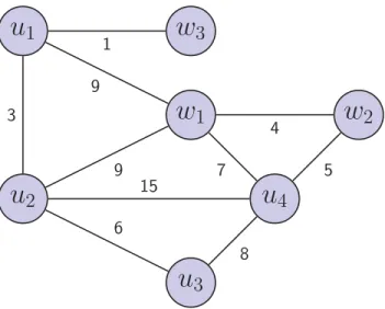
5.1 Weighted graph. . . 72

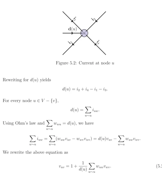
5.2 Current at nodeu . . . 82

6.1 Connected graph with six pages. . . 90

SUMMARY

A Markov chain on a finite or countable set of states is a stochastic process with the special property of ”memorylessness.” The sequence of states that the process transitions through is the Markov chain. Given any starting distribution and the probability transition matrix, we easily find the distribution after any number of transitions.

In Chapter 2, we study Markov chains with a single communication class and the additional property of recurrence. Such Markov chains eventually reach a stationary distribution. We relate irreducibility and recurrence of the Markov chain to irreducibility and primitivity of the probability transition matrix. The stationary distribution is then the left Perron vector of the probability transition matrix. Using the fundamental matrix of the Markov chain, we derive a formula for the hitting time between states.

In Chapter 3, we study a special kind of Markov chain, namely random walk on an undirected, unweighted, and connected graph. The main result in this chapter is a formula for the hitting time between vertices of the connected graph. We define a symmetric form of the probability transition matrix and find its spectral

decomposition. Using this spectra, we compute the hitting time and commute time between vertices of the graph.

If we look at the World Wide Web as a large but finite connected graph and a user browsing the web as taking a random walk on this graph, then the concepts developed in chapters 2 and 3 are easily applied to this web graph. Google’s

PageRank is the left Perron vector of a modified probability transition matrix, the Google matrix, designed to be primitive. In Chapter 4, we also mention a simple iterative algorithm for computing PageRank and how it translates to the large web graph.

The last two chapters draw an intriguing analogy between random walks on connected weighted graphs and electrical networks. In Chapter 5, drawing on the initial work of [AC96] and [PGD06], we relate the vertices of a graph to nodes in an electrical network and the edges of the graph to connectors between electrical nodes. In this context, the flow of electrons is similar to a random walk on the graph. Using harmonic functions, we establish that the voltage potential between nodes and hitting time between vertices are indeed the same function. Finally, in Chapter 6 we follow the work of [FC10] to modify the regular random walk and design a lazy random walk. The personalized PageRank is the stationary distribution of this lazy random walk. We study the normalized Laplacian of the lazy random walk and its inverse, the Green’s function. By linking voltage potential in an electrical network to the normalized Laplacian, we derive a direct formula for the hitting time in terms of the personalized PageRank.

CHAPTER 2

MARKOV CHAIN

A Markov chain, named after Andrey Markov (1856-1922), is a random process that transitions from one state to another, among a finite or countable number of possible states. It is a mathematical model for a random process evolving with time, usually characterized as memoryless: the next state depends only on the current state and not on the sequence of states that precede it. We say that the past affects the future only through the present. This specific kind of “memorylessness” is called the Markov property. The time can be discrete (integers), continuous (the real numbers), or a totally ordered set like English words.

Markov chains model many interesting phenomena such as virus mutation, the spread of epidemics, and more. The lack of memory property makes it possible to build probabilistic models and predict how a Markov chain may behave. In our study, we shall focus our attention exclusively on Markov chains with discrete time and a finite set of states. We follow [Nor98] in this chapter.

Example 2.0.1. Consider a mouse in a cage with two cells: cell 1 with ripe cheese and cell 2 with fresh cheese as shown in Figure 2.1. A scientist observes the mouse and records its position every minute. If the mouse is in cell 1 at minute n, then at minute n+ 1 it has either moved to cell 2 or stays in cell 1. Statistical observations led the scientist to conclude that the mouse moved from cell 1 to cell 2 with

probability α= 0.95. Similarly, when in cell 2 it moved to cell 1 with probability

β = 0.01. As we see, at any time, the mouse decides where to move only based on where it is now and not where it came from.

Figure 2.1: Cheesy dilemma

We represent the transition from cell 1 to cell 2 using aprobability transition

matrix P. In this scenario, P is a 2×2 matrix with the rows and columns indexed by 1 and 2 and each entry pij is the probability of the mouse moving from cell ito cell j. Since the mouse moves from cell 1 to cell 2 with probability α= 0.95, it stays in cell 1 with probability 1−α= 0.05. Similarly, it stays in cell 2 with probability 1−β = 0.99. The probability transition matrix is

P = ⎡ ⎢ ⎣1−α α β 1−β ⎤ ⎥ ⎦= ⎡ ⎢ ⎣0.05 0.95 0.01 0.99 ⎤ ⎥ ⎦.

2.1 Basic definitions and theorems

Definition 2.1.1. Stochastic process.

A stochastic process is a sequence of random variables (Xn)n≥0 having a common range in the finite state spaceI for the process.

Definition 2.1.2. Stochastic matrix.

A stochastic matrix is a nonnegative matrix [xij] in which each row sum equals 1;

j

xij = 1 for every row i of the matrix.

Definition 2.1.3. Markov chain.

distribution μand probability transition matrix P = [pij], if it satisfies the following properties:

i. the initial state X₀ has the initial distribution μ; that is P(X₀ =i) = μi for all i∈I.

ii. for n≥0,conditioning on Xn=in, Xn+1 has distribution (pinin+1 :in+1 ∈I) and is independent of X₀, X₁,· · · , Xn−1. We write this as

P(Xn+1 =in+1|X0 =i0,· · · , Xn=in) = pinin+1. (2.1)

We are interested in the special case of time-homogeneous Markov chains,

which means that the transition probabilities of pij(n, n+ 1) do not depend on n. From here on we consider only time-homogeneous and finite state Markov chains. Notation: M arkov(μ, P) represents a Markov chain with initial probability distribution μand probability transition matrix P.

Definition 2.1.4. n-step Transition probability.

The probability of transitioning from state i to statej in n time steps is given by P(Xn=j|X0 =i) = p(

n) ij .

p(_ijn) is the n-step transition probability fromi toj.

With these definitions, we are now ready to state our theorems on Markov chains.

Theorem 2.1.5. (_{Markov property}) A stochastic process (Xn)n≥0 is

Markov(μ, P) if for all states ik∈I, 0≤k ≤N

Proof. Suppose (Xn)n≥0 is Markov, applying Definition 2.1.3, the claim holds by the conditional independence of (Xn+1) and (X0, X1,· · · , Xn−1) given Xn.

Theorem 2.1.6. A stochastic process (Xn)n≥0 is Markov(μ, P) if and only if for all

states i₀, i₁,· · · , iN ∈I

P(X₀ =i₀, X₁ =i₁,· · · , Xn=in) =μi0pi0i1pi1i2· · ·pin−1in. (2.3)

Proof. Suppose (Xn)n≥0 is Markov(μ, P),then

P(X₀ =i₀, X₁ =i₁,· · · , Xn=in)

=P(X₀ =i₀)P(X₁ =i₁|X₀ =i₀)· · ·P(Xn=in|Xn₋₁ =in₋₁· · ·X₀ =i₀). (2.4)

By Markov property in Theorem 2.1.5, we have

P(Xk =ik|Xk₋₁ =ik₋₁· · ·X₀ =i₀) =P(Xk =ik|Xk₋₁ =ik₋₁). Applying this in (2.4), we get

P(X₀ =i₀)P(X₁ =i₁|X₀ =i₀)· · ·P(Xn=in|Xn−1 =in−1· · ·X0 =i0) =P(X₀ =i₀)P(X₁ =i₁|X₀ =i₀)· · ·P(Xn =in|Xn−1 =in−1). The transition probability from statei to j is given by pij. So, we get

P(X₀ =i₀, X₁ =i₁,· · · , Xn=in) =μi0pi0i1pi1i2· · ·pin−1in.

For the reverse, suppose (2.3) holds for alli∈I. By induction, we establish that P(X₀ =i₀, X₁ =i₁,· · · , Xn=in) =μi₀pi₀i₁pi₁i₂· · ·pi_n−1i_n.

From probability theory, we know that given two eventsA and B with P(A)>0, the conditional probability P(B|A) is given by

P(B|A) = P(A∩B) P(A) . Using this, we write

P(Xn₊₁ =in₊₁|X₀ =i₀,· · · , Xn =in) = P (X₀ =i₀,· · · , Xn₊₁ =in₊₁) P(X₀ =i₀,· · · , Xn =in) = μi0pi0i1pi1i2· · ·pin−1inpinin+1 μi0pi0i1pi1i2· · ·pin−1in =pi_ni_n+1. So (Xn)n≥0 is Markov.

Theorem 2.1.7. Suppose (Xn)n_≥0 is Markov(μ, P). Then

i. P(Xn =j) = (μTPn)j.

ii. P(Xn₊m =j|Xm =i) =p(ijn) where m, n are any two positive integers.

Note: Here p(_ijn) refers to the (i, j)th entry of the matrix power Pn_.

Proof. i. The probability that Xn =j is the sum of the probability of all possible paths starting at any state, based on the initial probability distributionμ, and navigating to state j after n−1 steps. We write this as

P(Xn=j) = P(X0 =i1)P(X1 =i2)· · ·P(Xn=j)+

· · ·+P(X₀ =in−1)· · ·P(Xn=j). (2.5) Writing this using summations notation and applying Theorem 2.1.6, we get

P(Xn =j) = i1∈I · · · in−1∈I μi₁pi₁i₂pi₂i₃· · ·pi_n−1j = [μTPn]j.

ii. The Markov property in Theorem 2.1.5 proves that the future states depend only on the current state and not the states that precede it. Given thatXm=i, the probability distribution after step m is μm _{= [0,0,· · · ,1,0,0], where 1 is in} the ith _{position. Using (i) above, we get}

P(Xn+m =j|Xm =i) = [(0,0,· · ·,1,0,0)·Pn]j =p( n) ij . We callp(_ijn) as the n-step transition probability from statei toj.

Lemma 2.1.8. Chapman-Kolmogorov equation. p(_ijm+n) =

k_∈I

p(_ikm)p(_kjn). Proof. Method 1. By Theorem 2.1.7 (ii),

p(_ijm+n) =P(Xm+n =j|X0 =i) = k∈I P(Xm =k, Xm+n=j|X0 =i) = k∈I P(Xm =k|X₀ =i)P(Xm₊n=j|Xm =k, X₀ =i) = k∈I p(_ikm)P(Xm₊n=j|Xm =k, X₀ =i) = k∈I p(_ikm)P(Xm+n=j|Xm =k), since (Xn)n≥0 is Markov = k_∈I p(_ikm)p(_kjn).

Method 2. By matrix multiplication, we havePm+n =PmPn. Thus,

p(_ijm+n) = [P(m+n)]ij = k∈I [Pm]ik[Pn]kj = k∈I p(_ikm)p(_kjn).

Corollary 2.1.9. Based on the above lemma we have these two results: i. p(_ijm+n)≥p_ik(m)p(_kjn), for any k∈I.

ii. p(_ija+b+c) ≥p_ik(a)p(_klb)p_lj(c), for any k, l∈I.

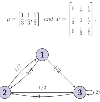
Example 2.1.10. Consider a three state, I ={1,2,3}, Markov chain (μ, P) as shown in Figure 2.2 with

μ= 1 3, 1 3, 1 3 and P = ⎡ ⎢ ⎢ ⎢ ⎢ ⎣ 0 1₂ 1₂ 1 2 0 12 0 1₃ 2₃ ⎤ ⎥ ⎥ ⎥ ⎥ ⎦.

1

2

3

Figure 2.2: State transition diagram.

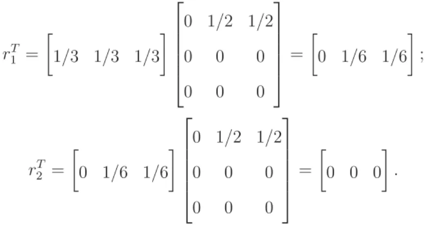
Using (2.5), we compute the probability that the chain is in state 1 at the second step as P(X₂ = 1) =P(X₀ = 1, X₁ = 2, X₂ = 1) +P(X₀ = 3, X₁ = 2, X₂ = 1) =P(X₀ = 1)P(X₁ = 2|X₀ = 1)P(X₂ = 1|X₁ = 2) +P(X₀ = 3)P(X₁ = 1|X₀ = 3)P(X₂ = 1|X₁ = 2) =μ(1)p₁₂p₂₁+μ(3)p₃₂p₂₁ = 1 3· 1 2· 1 2 + 1 3 · 1 3· 1 2 = 5 36 = μ T P2 1 .

Using Theorem 2.1.7 (ii), we compute the conditional probability P(X₅ = 3|X₂ = 1) as p(3)₁₃ = 1 0 0 P3 3 = 43 72. 2.2 Stationary distribution

Let (Xn)n≥0 be Markov(μ0, P) with state spaceI and let μk be the distribution of (Xn)n≥0 at step k.

μk_i =P(Xk=i) for all i∈I.

By conditioning on the possible predecessors of the (k+ 1)-th state, we see that

μk_j+1 =P(Xk+1 =j) = i_∈I P(Xk =i)pij = i_∈I μk_ipij for all j ∈I.

Rewriting this in vector form gives

[μk+1]T = [μk]TP fork ≥0.

Since P is stochastic and μ0 is a distribution, μk _{is a distribution for all k. Hence,} by Theorem 2.1.7

[μk]T = [μ0]TPk for k ≥0.

Does this sequence of distributions {μ0, μ1,· · · } have a limiting value? If such a limiting distribution π exists, then

πTPn+1 =πTPnP.

Hence, by taking limit,

Eigenvector interpretation: The equation πT _=πT_{P signifies that π is a left} eigenvector of the matrixP with eigenvalue 1. In addition, π must be a distribution:

i∈I

π(i) = 1.

The matrix P always has the eigenvalue 1 because P is stochastic, i.e.

j∈I

pij = 1.

In matrix notation we write this as P1=1, where 1 is a column vector whose entries are all 1; hence,1 is a (right) eigenvector of P corresponding to eigenvalue 1.

Definition 2.2.1. Stationary distribution.

A steady-state vector or stationary distribution for a finite state Markov chain with transition matrix P, is a vector π that satisfies

πT =πTP, where

i∈I

πi = 1 and πi ≥0, for all i∈I. (2.7)

Markov chain theory ensures that this sequence of distributions has a limiting stationary distribution for certain types of random processes. From

Perron-Frobenius Theorem B.0.22, we know that an irreducible and primitive matrix has such a limiting distribution. We now look at the conditions under which the probability transition matrix of a Markov chain is irreducible and primitive.

2.3 Irreducible Markov chain

Consider a Markov chain with state space I and probability transition matrix

P. Supposei, j are any two distinct states. We say that j is reachable from iif there exists an integer n≥0 such that p(_ijn) >0. Suppose iis also reachable from j, i.e., p(_jin)>0,for some positive integer n, then states iand j are said to

communicate with each other. We write this as i↔j. By convention, all states are

Theorem 2.3.1. Communication is an equivalence relation. 1. Reflexive: i↔i for all states i.

2. Symmetric: If i↔j, then j ↔i.

3. Transitive: If i↔j and j ↔k then i↔k.

Proof. Since P0 is the identity matrix,p(0)_ii = 1 for all statesi. Hence, i↔i for all states i.

Ifi↔j, then for some positive integersn, n, p_ij(n) >0 andp(_jin)>0. And if

j ↔k, then for some positive integersm, m, p_jk(m) >0 and p(_kjm) >0. By Chapman-Kolmogorov equation, we have

p(_ikn+m)= l∈I

p_il(n)p(_lkm) ≥p_ij(n)p(_jkm) >0.

Similarly, it is easy to show that p(_kin+m)>0 and so i↔k.

All states that communicate with each other belong to the same communication class and communication classes do not overlap. Thus, the communication classes partition the state space I.

Example 2.3.2. Consider a Markov chain onI ={1,2,3} with the following:

P = ⎛ ⎜ ⎜ ⎜ ⎜ ⎝ 1/2 1/2 0 1/2 1/4 1/4 0 1/3 2/3 ⎞ ⎟ ⎟ ⎟ ⎟ ⎠. Then P 2 ₌ ⎛ ⎜ ⎜ ⎜ ⎜ ⎝ 1/2 3/8 1/8 3/8 19/48 11/48 1/6 19/36 11/36 ⎞ ⎟ ⎟ ⎟ ⎟ ⎠.

Since P2 is a positive matrix, all states communicate and there is a single communication class.

Suppose we change the last row of the probability transition matrix as shown below: P = ⎛ ⎜ ⎜ ⎜ ⎜ ⎝ 1/2 1/2 0 1/2 1/4 1/4 0 0 1 ⎞ ⎟ ⎟ ⎟ ⎟ ⎠.

Then, Pn _{is not a positive matrix for any positive integern. P has two}

communication classes containing the appropriate states, namely C₁ ={1,2} and

C₂ ={3}.

Definition 2.3.3. Irreducible Markov chain.

A Markov chain for which there is only one communication class is called an

irreducible Markov chain; all states communicate.

Theorem 2.3.4. If M arkov(μ, P) is irreducible, then its probability transition matrix P is also irreducible.

Proof. Suppose M arkov(μ, P) is irreducible. Then for every pair of states

(i, j), i=j, there exists a positive integerk (depending oni, j) such that p(_ijk)>0.

Suppose matrix P is reducible. By Definition B.0.14,

UTP U = ⎡ ⎢ ⎣B C 0 D ⎤ ⎥ ⎦,

for some n×n permutation matrixU. Note that U UT _{=I. By matrix block}

multiplication, (UTPkU) = UTP U·UTP U· · · k times = (UTP U)k= ⎡ ⎢ ⎣B k _∗ 0 Dk ⎤ ⎥ ⎦. Clearly, [UT_Pk_U]

n₁ = 0. Since the 1st column and nth row ofU are the standard vectors ej, ei 0 = [UTPkU]n1 = [Urow nT ]P k_[U col1] =eTi P k_e j = [Pk]ij.

By irreducibility of the Markov chain, [Pk_] ij =p( k₎ ij >0, a contradiction. Hence, P is irreducible. 2.4 Recurrent states

The probability that the chain reenters statei after n steps is given by P(Xn=i|X₀ =i) = p(iin).

Consider the random variable

Ln= ⎧ ⎪ ⎪ ⎨ ⎪ ⎪ ⎩ 1, if Xn =i. 0, if Xn =i. Then, the number of visits to state i is

∞

n=0

Ln.

The expected value of the number of visits to i is given by

E(number of visits toi|X₀ =i) =E ∞ n=0 Ln = ∞ n₌₀ E(Ln|X₀ =i) = ∞ n=0 P(Ln= 1|X0 =i) = ∞ n=0 P(Xn =i|X0 =i) = ∞ n=0 p(_iin).

Definition 2.4.1. Recurrent state.

A state i is said to be recurrent if

∞ n=0 p(_iin) =∞; transient if ∞ n=0 p(_iin) <∞.

Theorem 2.4.2. For any communication classC, if a state i∈C is recurrent, then all states in C are recurrent. If not, all states are transient.

Proof. Suppose i∈C is recurrent. Let j ∈C. By definition of communicating class,

i↔j. So, there exists positive integers a, b such thatp(_ija) >0 and p(_jib) >0. Using Chapmann-Kolmogrov, we compute p(_jjn+a+b) ≥p_ji(b)p(_iin)p(_ija), for any n, and so k≥0 p(_jjk) ≥ a,b,n≥0 p(_jjn+a+b) ≥p(_jib)p(_ija) n≥0 p(_iin) =∞.

Hence, j is also recurrent. Since this is true for any j ∈C, all states in C are recurrent.

Definition 2.4.3. Recurrent Markov chain.

If all states in a Markov chain are recurrent, then the Markov chain is termed recurrent; it is transient otherwise.

Proof. LetI ={ik},1≤k ≤m, be the set of possible states of the Markov chain. We start by generating a sequence of non-communicating states. If state i₁ is transient, then there exists state i₂ such that i₁ →i₂ but i₂ →i₁. If i₂ is also transient, then for some statei₃,i₂ →i₃ but i₃ →i₂ and i₃ =i₁. Thus, successive states, i₁, i₂,· · · , ik are distinct and transient. If for some state ik+1, ik→ik+1 but

ik+1 →ik, then ik+1 =ij for 1≤j ≤k.

Suppose the Markov chain is in stateik+1 having visited all other states in I but without revisiting any state. Then, in the next step, the chain must re-visit some state ij,1≤j ≤k. So, p(k+1)j >0. The chain then revisits the sequence of states {ij, ij+1,· · · , ik, ik+1}. So, there is a path from ij →ik+1, k > j and

pn_j(k+1)>0 for some positive integer n. So, j ↔(k+ 1) and states j and k+ 1 communicate. By transitivity of ↔, this sequence of states {j, j + 1,· · · , k, k+ 1} form a communication class. It is now easy to see that

∞

n₌₀

p(₍n_k+1)() _k+1) =∞,

and statek+ 1 is recurrent. By Theorem 2.4.2, all states in this communication class are recurrent. Hence, a finite state Markov chain cannot have all transient states.

Corollary 2.4.5. An irreducible and finite state Markov chain has all recurrent states.

Proof. From Theorem 2.4.4, the Markov chain must have at least one communication class with recurrent states. But the chain is irreducible. By

Definition 2.3.3, it has only one communication class. Since all states communicate, the chain revisits all states. So, all states are recurrent.

2.5 Periodic and aperiodic Markov chains

Definition 2.5.1. Period of a Markov chain.

The period r(i) of a recurrent state i∈I is defined to be the greatest common divisor of all steps n at which the Markov chain returns to i.

D(i) ={n∈Z+|p(_iin) >0}. r(i) =gcd D(i) .

Theorem 2.5.2. If two states i, j ∈I communicate, then r(i) = r(j).

Proof. Suppose two states, i, j ∈I, communicate. Then, for some positive integers

x, y, p(_ijx)>0, p(_jiy) >0, and p(_jjx+y) ≥p_ji(y)p(_ijx) >0. Hence, r(j)|(x+y).If n∈D(i) is such that p(_iin) >0, then p(_jjx+y+n) ≥p(_jiy)p_ii(n)p(_ijx)>0. Hence, r(j)|(x+y+n). A number that divides any two numbers must divide their difference as well, so

r(j)|n for all n∈D(i). Sincer(i) is the gcd ofD(i), we must have r(j)≤r(i). Similarly, it is straightforward to show that r(i)≤r(j). Hence, r(i) =r(j).

Corollary 2.5.3. Period is a class property.

Corollary 2.5.4. An irreducible and recurrent Markov chain has the same period for all states i∈I.

Proof. An irreducible Markov chain has a single communication class. By Theorem 2.5.2, all states have the same period.

Definition 2.5.5. Aperiodic Markov chain.

An irreducible, recurrent Markov chain with period one is aperiodic.

Theorem 2.5.6. If an irreducible Markov chain is aperiodic, its probability transition matrix P is primitive.

Proof. A matrix P is primitive, if for some positive integerL, PL is a positive matrix as defined in B.0.13.

Suppose (Xn)n≥0 Markov(μ, P) is irreducible and aperiodic. By Lemma D.0.40, for every statei, there exists m_i ∈M_i such that for anym ≥m_i, p(_iim)>0. Set

M =maxi_∈I(mi).

By irreducibility of the Markov chain, for every pair (i, j), i=j, there exists

rij ∈Z+, such that p( r_ij)

ij >0. Set R =maxi,j_∈I,i₌j(rij).

LetL=M +R. Then, for every state i,L≥mi. So, p(iiL) >0. For every pair (i, j),

L≥rij +mi.Hence, p(ijL) ≥p (L−r_ij) ii p (r_ij) ij ≥p( mi) ii p (r_ij) ij >0. Thus, P is primitive.

Theorem 2.5.7. Suppose M is a stochastic matrix. Then the spectrum of M is contained in the unit disc.

Proof. Letv be an eigenvector of M and λ the corresponding eigenvalue. Then for any matrix norm || · ||, by Theorem 5.6.8 in [RAH85], we have

|λ|||v||=||λv||=||M v|| ≤ ||M||||v||.

Since v is a nonzero vector,

|λ| ≤ ||M||∞ = 1,

where || · ||∞ is the max row sum norm. Hence, the eigenvalues of the probability transition matrix P lie in [−1,1].

Theorem 2.5.8. _{The fundamental stability theorem for Markov chains.} Suppose M arkov(μ, P) is irreducible and aperiodic. Then

i. M arkov(μ, P) has an unique stationary distribution π.

ii. The probability transition matrix P converges to a matrix with rows all equal to πT. lim m→∞P m _=1πT _{where lim} m→∞p (m) ij =π(j), i, j ∈I. iii. lim

m→∞P(Xm =j) =π(j), for any initial distribution μ.

Proof. By Theorem 2.5.6,P is primitive. So, we apply the Perron-Frobenius

Theorem B.0.22 to P.

i. P has only one eigenvalue λ >0 on its spectral radius. By Theorem 2.5.7,

λ= 1 is the spectral radius of P. Hence,λ = 1 is the largest, simple eigenvalue

ofP. By Perron-Frobenius Theorem, P has unique left and right Perron vectors

corresponding to λ. Since P is stochastic, we see that 1 is the right eigenvector with eigenvalue 1. Suppose we denoteπ to be the left eigenvector. By

Perron-Frobenius Theorem, we know that πT₁₌

n

i=1

π(i) = 1. Thus, π is a probability distribution. Since πT_{P =π}T_{, by Definition 2.2.1, π is the unique} stationary distribution vector of P.

1 and are strictly positive. By Perron-Frobenius Theorem iv,P has a limit lim m→∞[P] m _=1πT ₌ ⎡ ⎢ ⎢ ⎢ ⎢ ⎢ ⎢ ⎢ ⎣ π₁ π₂ · · · πn π₁ · · · · πn .. . ... π₁ π₂ · · · πn ⎤ ⎥ ⎥ ⎥ ⎥ ⎥ ⎥ ⎥ ⎦ . iii. By 2.1.7(ii), P(Xm =j) =p( m) ij . By 2.1.8, p (m)

ij = [Pm]ij. Using (ii) above, we have the desired result.

For Markov chains, the past and the future are independent of the present. This property is symmetrical in time and suggests we look at the reverse of a Markov chain, running backwards. But we have looked at Markov chains that converge to a limiting invariant distribution. This suggests that if we start with the invariant distribution, the Markov chain will be in equilibrium, i.e., a Markov chain running forward and backward are symmetric in time. A Markov chain running backwards is also a Markov chain, but with a different probability transition matrix.

Theorem 2.5.9. Let P be irreducible with π as its stationary distribution. Suppose

(Xn) is Markov. Set Yn=XN₋n, for some fixed N. The reverse chain (Yn) is also

Markov(π,Pˆ), where Pˆ = [ˆpij] is given by

πjpˆji =πipij for all i, j ∈I. (2.8)

Furthermore, Pˆ is also irreducible with stationary distribution π. Proof. First, we show that ˆP is stochastic. ˆpji = _ππi

jpij. We write ˆP as

ˆ

where D(π) is the diagonal matrix with πi on the diagonals and D(π−1) is the diagonal matrix with 1/πi on the diagonals. Then

ˆ

P1= [D(π−1)PTD(π)]1=D(π−1)PTπ=D(π−1)π=1.

Next, we show that (Yn) is Markov.

P(Y₀ =i₀, Y₁ =i₁,· · · , YN =iN)

=P(XN =iN, XN−1 =iN−1,· · · , X0 =i0) =πi_Npi_Ni_N−1pi_N−1i_N−2· · ·pi1i0

=πi₀pˆi₀i₁pˆi₁i₂· · ·pˆi_N−1i_N. By Theorem 2.1.6, (Yn) is Markov(π,Pˆ).

To show that ˆP is also irreducible, consider any two distinct states i, j. There exists a chain of states i₀ →i₁ → · · · →ik and pi₀i₁· · ·pi_k−1i_k >0. Then

ˆ

pi_Ni_N−1· · ·pˆi_N−k−1i_N−k = 1

πi_N

πi₀pi₀i₁· · ·pi_k−1i_k >0. So, there is only one communication class. Hence, ˆP is also irreducible. Finally, we show that π is indeed the stationary distribution of ˆP.

πTPˆ=πT[D(π−1)PTD(π)] =1TPTD(π) =1TD(π) =πT. (2.9)

Definition 2.5.10. Time-reversed Markov chains.

The chain (Yn)n_≥0 is called the time-reversal of (Xn)n_≥0.

Definition 2.5.11. Detailed balance.

balance if ˆP =P, i.e.

D(π)P =PTD(π)

P =D(π−1)PTD(π) = ˆP .

We write the condition in (2.8) asπjpji =πipij.

Example 2.5.12. Consider a Markov chain with state transition diagram as shown in Figure 2.3. πT = _{1/3 1/3 1/3} and P = ⎡ ⎢ ⎢ ⎢ ⎢ ⎣ 0 2/3 1/3 1/3 0 2/3 2/3 1/3 0 ⎤ ⎥ ⎥ ⎥ ⎥ ⎦. ˆ P =D(π−1)PTD(π) = ⎡ ⎢ ⎢ ⎢ ⎢ ⎣ 0 1/3 2/3 2/3 0 1/3 1/3 2/3 0 ⎤ ⎥ ⎥ ⎥ ⎥ ⎦.

1

2

3

1

2

3

Figure 2.3: Markov chain not in detailed balance P = ˆP .

Example 2.5.13. Consider a Markov chain with state transition diagram as shown below in Figure 2.4.

4

1

2

3

Figure 2.4: Markov chain in detailed balanceP = ˆP .

πT ₌ 1/5 3/10 1/5 3/10 and P = ⎡ ⎢ ⎢ ⎢ ⎢ ⎢ ⎢ ⎢ ⎣ 0 1/2 0 1/2 1/3 0 1/3 1/3 0 1/2 0 1/2 1/3 1/3 1/3 0 ⎤ ⎥ ⎥ ⎥ ⎥ ⎥ ⎥ ⎥ ⎦ = ˆP .

2.6 Hitting time of a connected graph

Definition 2.6.1. Hitting time.

Given an irreducible and aperiodic Markov chain (Xn)n≥0, and two distinct states

i, j ∈I, the hitting time ormean first passage time is the expected number of steps to reach state j starting from state i, for the first time.

H(i, j) =

∞

t=1

t·P(Xt=j|X0 =i, Xk =j, k < t).

Definition 2.6.2. Return time.

Given an irreducible and aperiodic Markov chain (Xn)n≥0, and state i∈I, the

for the first time. R(i) = ∞ t=1 t·P(Xt=i|X0 =i, Xk =i, k < t).

Since there are numerous paths from i→j, the probabilistic computation of hitting time and return time is laborious. So, we look at matrix based techniques for simplifying such computations. Consider the first step to any statek fromi with

pik >0. Then from k we navigate toj. We write this as

H(i, j) = 1 + k=j

pikH(k, j). (2.10)

Similarly, starting at i, the chain takes at least one step to some statej =i

and returns to i. Considering all possible first steps, we get

R(i) = k pik(H(k, i) + 1) = 1 + k pikH(k, i). (2.11)

Define two matrices H, where Hij =H(i, j), Hii = 0 andR, a diagonal matrix with Rii=R(i). We combine the above two equations in to a single matrix form as

H=PH+J−R,where J is the all one matrix. (2.12)

Equivalently,

(I−P)H=J −R. (2.13)

Theorem 2.6.3. If M arkov(μ, P) is irreducible and aperiodic, then the return time for any state i∈I is R(i) = 1/π(i), where π is the stationary distribution.

Proof. Multiplying both sides of (2.13) by πT _gives

πT(I−P)H=πTJ−πTR.

Since πT_{P =π}T _{and π}T_{J =1}T_{, we get}

yielding R(i) = 1/π(i) for all statesi.

2.6.1 Fundamental matrix

The matrix (I−P) is not invertible, since it has row sum zero. So, we consider a rank-one update Π =1πT _{to (I−P). The new matrix (I−P + Π) is} invertible. We define Q= (I−P + Π)−1 to be the fundamental matrix of the

Markov chain. We now look at some properties of the fundamental matrix Q.

Proposition 2.6.4. QJ =J.

Proof. Since P J =J and ΠJ =J, (I−P + Π)J =J. Hence, QJ =Q(I−P + Π)J

gives us QJ =J. Proposition 2.6.5. Q1=1. Proof. Since (I−P + Π)1=1, 1=Q1. Proposition 2.6.6. Q(I−P) = (I−P)Q= (I−Π).

Proof. Note thatPΠ =P1πT _=1πT _{= Π. Similarly, ΠP =1π}T_{P =1π}T _{= Π.} Also, Π2 =1(πT_1)πT _=1πT _{= Π. So, we have,}

And

(I−Π)(I−P + Π) = I−Π−P + Π + Π−Π = (I−P).

Hence, Q(I−P) = (I−P)Q= (I −Π).

Theorem 2.6.7. The hitting time in terms of the fundamental matrix Q is given by

Hij =

Qjj−Qij

πj

.

Proof. From (2.13), we have

(I−P)H=J −R.

Multiplying on the left by Q yields

Q(I −P)H=Q(J −R).

From propositions 2.6.4 and 2.6.6, we get (I−Π)H=J−QR. Hence

H=J −QR+ ΠH. (2.14)

So,

0 =Hjj = 1−QjjR(j) + [πTH]j, (2.15)

and

Hij = 1−QijR(j) + [πTH]j. (2.16)

Subtracting (2.15) from (2.16) results in

Substituting R(j) = 1/π(j), allows us to express the hitting time between any two distinct states as Hij = Qjj−Qij πj . (2.17)

CHAPTER 3

RANDOM WALK ON GRAPHS

A random walk is a mathematical formalization of a path that consists of a succession of random steps. For example, the path traced by a molecule as it travels in liquid or gas, the search path of a foraging animal, the price of a fluctuating stock, or the financial status of a gambler can all be modeled as random walks, although they may not be truly random in reality. The term random walk was first introduced by Karl Pearson in 1905. Random walks have been used in many varied fields: ecology, economics, psychology, computer science, physics, chemistry, biology, finance, and more. Random walks explain the observed behaviors of processes in these fields and thus serve as a fundamental model for the recorded stochastic activity. Though many types of random walks exist, we are interested in random walks that are time-homogeneous Markov chains. Random walks occur on graphs, integer lines, planes, or even on topological structures of higher dimensions. Our study focuses on time-homogenous random walks on finite, connected graphs. Appendix C contains basic definitions and theorems on graphs.

In this chapter we follow [Lov93].

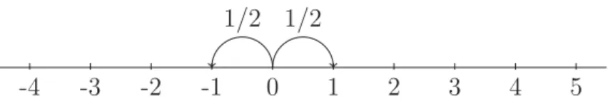
Example 3.0.8. Let us consider a simple random walk on the integer line as shown in Figure 3.1.

Suppose our random walk starts on 0. The probability of getting to 1 and −1

are the same, equal to 1₂. This is true for the transition from any integern ton±1. This is an example of a simple random walk and is sometimes referred to as the drunkard’s walk.

-4 -3 -2 -1 0 1 2 3 4 5 1/2 1/2

Figure 3.1: Drunkard’s walk on an integer line.

3.1 Random walk on graphs

Given a finite, connected graph G(V, E), and a starting vertex v₀, choose any adjacent vertexv₁ at random and move to this neighbor. Then select v₂, a neighbor of v₁ at random and move to v₂, and so on. The sequence of vertices, so chosen,

{v₀, v₁,· · · , vk}, constitute a random walk onG.

At each step k, we assign to the random variableXk, a value from V. Hence, the random sequence X₀, X₁, X₂,· · ·Xk,· · · ,is a discrete time stochastic process defined on the state space V.

The choice of vertexvi, at any stepk, depends only on reaching its neighbor

vj in step (k−1) and not howvj is reached. In an unweighted graph, the

probability of taking an edge depends only on the degree of the current vertex and is the same for all edges from a vertex. Supposed(vi) denotes the degree of vertexvi and pij denotes the probability of moving from vertexvi to vertexvj. Then

pij =P(Xk₊₁ =vj|Xk =vi) = ⎧ ⎪ ⎪ ⎨ ⎪ ⎪ ⎩ 1 d(vi), if (ij)∈E. 0, otherwise.

The transition probabilities pij are independent of time k. If at time k we are at vertex vi,we choose vj uniformly from the neighbors of vi and move to it. The process is thus “memoryless;” the future choice of vertex depends only on the current vertex. We denote vi ∼vj if vj is a neighbor of vi. In this chapter, we focus on finite, connected, unweighted graphs.

Definition 3.1.1. Adjacency matrix.

For a graph G with V ={v₁, v₂,· · · }, the adjacency matrix A is given by

[A]ij = ⎧ ⎪ ⎪ ⎨ ⎪ ⎪ ⎩ 1, if vi ∼vj. 0, otherwise.

Definition 3.1.2. Degree matrix.

For a graph G, the degree matrix Dis the diagonal |V| × |V| matrix given by [D]ii =d(vi), where d(vi) =

j [A]ij.

Definition 3.1.3. Probability transition matrix.

For a graph G, the probability transition matrix P is the |V| × |V|matrix given by

P =D−1A.

Suppose μ0 is the initial probability distribution, the random sequence of vertices visited by the walk X₀, X₁,· · · , Xk,· · · , is M arkov(μ0, P) with state space

V. The probability distribution μt at any time t is given by [μt]T = [μ0]TPt.

Theorem 3.1.4. A random walk on a graph G with probability transition matrix P is Markov and Theorem 2.1.5 holds; i.e.,

P(Xk+1 =vj|Xk =vi, Xk−1 =vk−1,· · ·, X1 =v1, X0 =v0)

=P(Xk₊₁ =vj|Xk =vi) =pij. (3.1)

Proof. First, we show that the probability transition matrix P = [pij] of a random walk is stochastic. For any row i of the matrix P,

j pij = v_j∼v_i 1 d(vi) = 1,

since there are d(vi) entries in each rowi. To see that the Markov property holds, we use the definition ofP(A|B) and compute

P(Xk+1 =vj|Xk =vi, Xk−1 =vi_k−1,· · · , X0 =v0) = pijp(k−1)ip(k−2)(k−1)· · ·

p₍k−1)ip(k−2)(k−1)· · · =pij.

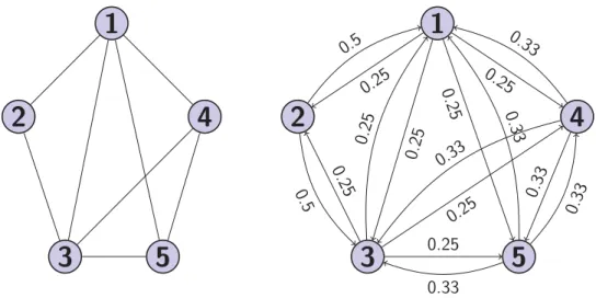
Example 3.1.5. Let us consider an undirected, connected graph with five vertices as shown in Figure 3.2. The probability of transition between any two vertices depends on the degree of the current vertex.

4

1

2

3

5

4

1

2

3

5

P = ⎡ ⎢ ⎢ ⎢ ⎢ ⎢ ⎢ ⎢ ⎢ ⎢ ⎢ ⎢ ⎣ 0 1₄ 1₄ 1₄ 1₄ 1 2 0 12 0 0 1 4 14 0 14 14 1 3 0 13 0 13 1 3 0 13 13 0 ⎤ ⎥ ⎥ ⎥ ⎥ ⎥ ⎥ ⎥ ⎥ ⎥ ⎥ ⎥ ⎦ .

We are interested in finding the stationary distribution of a random walk. From Markov chain theory, we know that if a Markov chain is irreducible and aperiodic, then the stationary distribution exists. The properties of the random walk reflect the properties of the underlying graph. Here, we show that a random walk on a connected, non-bipartite graph has a stationary distribution.

Theorem 3.1.6. A random walk on a connected graph G is irreducible.

Proof. Since the graph G is connected, for any two vertices vi, vj ∈V, there exists a path fromvi tovj: vi →vi₁ → · · · →vj such that pi_ki_k+1 >0 for every vertex vi_k in the path. The transition probability fromvi →vj is

P(Xm =vj|X₀ =vi) = P(Xm =vj|Xm₋₁ =vi_m−1, Xm₋₂ =vi_m−2,· · · , X₀ =vi)

≥pii₁pi₁i₂· · ·pi_m−1j >0.

The final step above is using Theorem 2.1.7. Similarly, there is a path from vj to vi. Sovi and vj communicate: vi ↔vj. By Theorem 2.3.1, communication is an

equivalence relation. Since graphG is connected, we conclude that all vertices in G communicate and hence belong to the same communication class. By Definition 2.3.3, the random walk is irreducible and by Theorem 2.3.4, the probability

Since the graph is connected, by Theorem 2.5.2 and its Corollary 2.5.4, all

vertices in G have the same period. Our next theorem shows that a random walk on

a non-bipartite graph is aperiodic.

Theorem 3.1.7. A random walk on a finite, connected graph is aperiodic if and only if the graph is non-bipartite.

Proof. From Appendix C.0.38, a graph is bipartite if and only if it has no odd cycles. Suppose the walk is aperiodic, by definition of aperiodic, the graph has an odd cycle, or else two divides its period. Hence the graph is not bipartite.

On the other hand, suppose the graph is non-bipartite, it has at least one odd cycle. Any random walk on a connected, undirected graph has a walk with return time of two, i.e., you leave a vertex in any direction and return back in the next step. So, for each vertex, the walk also has a cycle of length two. Hence the gcd of the set of cycles of G is one. By Definition 2.5.1, the graph is aperiodic.

Theorem 3.1.8. The stationary distribution vector π for a random walk on a finite connected graph G(V, E) exists and is given by πi =

d(vi)

2m , where m=|E|.

Proof. A random walk on a finite, connected graph is irreducible and aperiodic. By the fundamental stability theorem of Markov chains, Theorem 2.5.8, such a random walk has a stationary distribution and its probability transition matrix has a

limiting value. Furthermore, by Perron-Frobenius theorem, P has right and left

• πT _=πT_{P and π}T_{1= 1,}

• lim

m→∞P

m _{= Π = 1π}T_.

Suppose πi = d₂(_mvi) for all vi ∈V, it is easily verified that πTP =πT.

πTP = 1 2m[d(v1)· · ·d(vk)]D −1_A = 1 2m[1· · ·1]A = 1 2m[d(v1)· · ·d(vk)] =πT.

Theorem 3.1.9. A random walk on a finite, connected graph G is time reversible. Proof. From Definition 2.5.11, a Markov chain is time reversible if ˆP =P.

D(π−1)PTD(π) = 2mD−1(D−1A)TD 1

2m =D

−1_AT_D−1_D=D−1_A=P.

The random walk is in detailed balance. Hence is time reversible.

3.2 Access times on graphs

In a random walk, given any starting vertex, we choose any neighbor at

random and proceed. This random choice is distributed evenly among the neighbors of the said vertex. For a finite, connected graph, there is a path between any two arbitrary vertices. This allows us to turn our focus to less qualitative questions; rather than asking whether or not a random walk will return to its starting vertex,

it is interesting to ask what is the expected number of steps the random walk would take to return to the starting vertex, reach a specific vertex, or to commute between any two vertices.

Definition 3.2.1. Hitting time.

Given graph G, the hitting time H(i, j), i=j, from vertex vi tovj, is the expected number of steps it takes for a random walk that starts at vertex vi to reach vertex

vj for the first time.

H(i, j) =

∞

t=1

t·P(Xt=j|X0 =i;Xk =j, k < t).

Definition 3.2.2. Commute time.

Given graph G, the commute time C(i, j), i=j, between two vertices vi and vj is the expected number of steps that a random walk starting at vi takes to reach vj and return back to vi.

C(i, j) =H(i, j) +H(j, i).

Usually, H(i, j)=H(j, i). But C(i, j) = C(j, i). Definition 3.2.3. Return time.

Given graph G, the return time to a vertex R(i, i), is the number of steps that a random walk starting at vi takes to return tovi. Indeed, by Theorems 2.6.3 and 3.1.8, R(i, i) =πi−1 =

2m d(vi)

.

Example 3.2.4. Let us look at a simple random walk on a path with n+ 1 nodes:

{0,1,2,· · ·n}. We are interested in finding the hitting time H(i, k), where i and k

are any two nodes on the path. For k≥1, the hitting timeH(k−1, k), is equivalent

to the expected return time of a random walk on a path withk+ 1 nodes, starting

return to node k, it takes one fewer steps than had we started on node k. The

return time for any node is given by 2m

d(vi)

. The degree of the last node is one. Here we have k edges. Hence the return time is 2k. Hence H(k−1, k) = 2k−1.

Now, let us look at hitting time H(i, k),0≤i≤k ≤n. To reach node k, we first have to first reachk−1. So we have the recurrence

H(i, k) = H(i, k−1) + 2k−1 =H(i, k−2) + 2k−3 + 2k−1 =· · · =H(i, i+ 1) + (2i+ 3) +· · ·+ (2k−1) = (2i+ 1) + (2i+ 3) +· · ·+ (2k−1) = (k−i)(2i) + (1 + 3 +· · ·+ 2(k−i)−1) = 2ki−2i2+ (k−i)2 =k2−i2 In particular H(0, n) =n2.

Example 3.2.5. LetC be a cycle with n vertices. Then, the hitting time from any vertex vi to a vertex that is l steps away is independent of vi and is given by

H(i, i+l) = Hl =l(n−l).

Proof. From vertex vi, the first step is either to vertex vi−1 orvi+1, both with probability 1₂. H(i, i+l) = 1 2(H(i−1, i+l) +H(i+ 1, i+l)) + 1 = 1 2(H(i−1, i+l) + 1 2(H(i+ 1, i+l)) + 1 (3.2)

Since H(i, i+l) does not depend on i, but only on the distancel, we denote this by Hl and write Hl= 1 2Hl−1+ 1 2Hl+1+ 1 −1 = 1 2Hl−1+ 1 2Hl+1−Hl

We now setup a system of linear equations for l= 1, l= 2, etcetra.

1 2H0+ 1 2H2−H1 =−1 1 2H1+ 1 2H3−H2 =−1 1 2H2+ 1 2H4−H3 =−1 .. . 1 2Hn−2 + 1 2Hn−Hn−1 =−1

The above set of equations are linearly independent. Suppose a linear combination of the above n−2 equation must result in 0. SinceH₀ appears only in the first equation, that equation must have coefficient e₁ equal to 0 so that e₁H₀ equals 0.

Then, H₁ appears only in the second equation, hence this equation too must have

coefficient e₂ equal 0 so that e₂H₁ is 0. Proceeding in a similar manner, the coefficients of all the equation must be 0 to add up to 0. Hence this system must have an unique solution. We now verify Hl =l(n−l) is indeed the right solution by checking (3.2). The length of the path (i−1, l+i) = l+ 1 and the length of

(i+ 1, l+i) is l−1. H(i, i+l) = 1 2((l+ 1)(n−(l+ 1)) + 1) + 1 2((l−1)(n−(l−1)) + 1 = 1 2(nl+n−l 2_{−2l−2 + 1 +nl−n−l}2_{+ 2l−2 + 1) + 1} =nl−l2 =l(n−l).

Example 3.2.6. Consider a complete graph on vertices (0,1,· · ·, n−1). The hitting time is given byH(i, j) = n−1.

Proof. Since all vertices are connected to each other, it is sufficient to find H(0,1).

The probability that we choose vertex v₁ from any other vertex is 1

n−1. Then for every step that we do not choose v₁, we choose any other vertex with probability

n−2

n−1.Putting these together, the probability that we start at vertex v0 and reach vertex v₁ int steps is given by

P(Xt =v1|X0 =v0, Xk =v1 for k < t) = 1 n−1 n−2 n−1 t−1 .

The hitting time H(0,1) is

H(0,1) = ∞ t=1 t· 1 n−1 n−2 n−1 t−1 =n−1.

We take advantage of geometric series to prove this. Let S=H(0,1).

S = ∞ t=1 t· 1 n−1 n−2 n−1 t−1 = 1 n−1+ 2 n−1 n−2 n−1+ 3 n−1 n−2 n−1 ₂ +· · · n−2 n−1S = 1 n−1 n−2 n−1+ 2 n−1 n−2 n−1 ₂ + 3 n−1 n−2 n−1 ₃ +· · · S− n−2 n−1S = 1 n−1+ n−2 n−1 1 n−1+ n−2 n−1 ₂ 1 n−1 + n−2 n−1 ₃ 1 n−1 +· · · 1 n−1S = 1 n−1+ n−2 n−1 1 n−1 1 + n−2 n−1 + n−2 n−1 ₂ +· · ·

For 0< r <1, the geometric sum (1 +r+r2 +· · ·) is given by 1

1−r. If we set r= n_n−₋2₁, then the sum

1 n−1S = 1 n−1 1 + n−2 n−1+ n−2 n−1 ₂ +· · · = 1 n−1 1 1− n−2 n−1 = 1.