2015
Validation and application of close-range
photogrammetry to quantify ephemeral gully
erosion
Karl Richard Gesch Iowa State University
Follow this and additional works at:https://lib.dr.iastate.edu/etd
Part of theAgricultural Science Commons,Agriculture Commons,Agronomy and Crop Sciences Commons,Geomorphology Commons, and theSoil Science Commons
This Thesis is brought to you for free and open access by the Iowa State University Capstones, Theses and Dissertations at Iowa State University Digital Repository. It has been accepted for inclusion in Graduate Theses and Dissertations by an authorized administrator of Iowa State University Digital Repository. For more information, please [email protected].
Recommended Citation
Gesch, Karl Richard, "Validation and application of close-range photogrammetry to quantify ephemeral gully erosion" (2015).
Graduate Theses and Dissertations. 14319.
Validation and application of close-range photogrammetry to quantify ephemeral gully erosion
by
Karl Richard Gesch
A thesis submitted to the graduate faculty
in partial fulfillment of the requirements for the degree of MASTER OF SCIENCE
Major: Soil Science Program of Study Committee: Richard Cruse, Major Professor
Lee Burras Mark Tomer
Iowa State University Ames, Iowa
2015
TABLE OF CONTENTS
Page
LIST OF TABLES iv
LIST OF FIGURES v
LIST OF ABBREVIATIONS vi
LIST OF SYMBOLS vii
ACKNOWLEDGEMENTS viii
ABSTRACT ix
CHAPTER 1. IMPROVED MEASUREMENTS OF EPHEMERAL GULLY
EROSION WILL ENCHANCE SOIL CONSERVATION 1
Introduction 1
References 7
CHAPTER 2. QUANTIFYING UNCERTAINTY OF MEASURING GULLY
MORPHOLOGICAL EVOLUTION WITH CLOSE-RANGE DIGITAL
PHOTOGRAMMETRY 12 Abstract 12 Introduction 13 Methods 17 Results 24 Discussion 26 Conclusions 32 References 33
CHAPTER 3. A MULTI-TEMPORAL GEO-REFERENCED TOPOGRAPHIC
DATASET OF UPLAND EPHEMERAL CHANNEL DEVELOPMENT 47
Abstract 47
Introduction 47
Methods 52
Study Site 52
Photogrammetry & Post-Processing 53
Soil Properties 54
Ephemeral Gully Erosion 56
Results 58
Discussion 59
Conclusions 65
CHAPTER 4. EPHEMERAL GULLY EROSION AND SOIL
CONSERVATION 90
Conclusion 90
LIST OF TABLES
Page
Table 2.1. Point cloud uncertainty measures 37
Table 3.1. Monitoring sites and dates of photography 72
Table 3.2. Experimental watershed topographic characteristics 73
Table 3.3. Bulk density by block 74
Table 3.4. Measured soil properties 75
Table 3.5. Estimated ephemeral gully erosion, first time interval 76 Table 3.6. Estimated ephemeral gully erosion, second time interval 77 Table 3.7. Estimated ephemeral gully erosion, third time interval 78 Table 3.8. Estimated ephemeral gully erosion, fourth time interval 79
LIST OF FIGURES
Page
Figure 2.1. Experimental reach schematic 38
Figure 2.2. Camera station configuration 39
Figure 2.3. Point cloud of experimental reach 40
Figure 2.4. Nine image pairs 41
Figure 2.5. Schematic of nearest neighbor algorithm 42
Figure 2.6. Histogram of volume change 43
Figure 2.7. Histogram of average elevation error 44
Figure 2.8. Histogram of elevation discrepancy 45
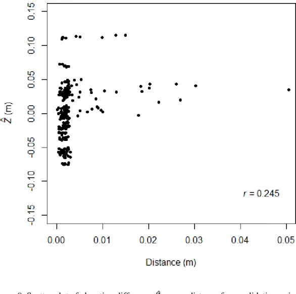
Figure 2.9. Scatter plot of elevation difference versus VP-NN distance 46
Figure 3.1. Location of study site 80
Figure 3.2. Identification of monitoring sites in Interim 3 81
Figure 3.3. Ground control point placement 82
Figure 3.4. Stereo image pair for Interim 3 Site 6 at T0 83
Figure 3.5. Matching points and camera sensors 84
Figure 3.6. Point cloud for Interim 3 Site 6 at T0 85
Figure 3.7. Stereo image pair and point cloud for Interim 3 Site 6 at T2 86 Figure 3.8. Elevation changes T0 to T2 within Interim 3 Site 6 87 Figure 3.9. Cross-section profile extracted during post-processing 88 Figure 3.10. Schematic of modified EAM interpolation procedure 89
LIST OF ABBREVIATIONS AnnAGNPS Annualized Agricultural Non-Point Source
CREAMS Chemicals, Runoff, and Erosion from Agricultural Management Systems
DEM digital elevation model
EAM end area method
EGEM Ephemeral Gully Erosion Model EphGEE Ephemeral Gully Erosion Estimator GCP ground control point
IaRTN Iowa Real-Time Network IDEP Iowa Daily Erosion Project LiDAR light detection and ranging MAE mean absolute error
NN nearest neighbor
RMS root mean square
RMSE root mean square error
RTK-GPS real-time kinematic global positioning system RUSLE2 Revised Universal Soil Loss Equation 2 SIFT scale-invariant feature transform
VP validation point
LIST OF SYMBOLS Bb bank, bottom Bt bank, top Con control Cb channel, bottom Ct channel, top
εΔZ vertical change error
ΔM mass flux
δΔM mass flux uncertainty
μ mean
ρb bulk density
σ sample standard deviation Ti time corresponding to i
ΔV volume change
ΔVc total channel volume change δΔV volume change uncertainty
𝑍̂ elevation difference
δΔZ elevation change uncertainty
δZgeo-ref absolute vertical accuracy
ACKNOWLEDGEMENTS
Many people have helped and encouraged me as I have explored the world of soil science. I am deeply grateful to Rick Cruse, not only for giving me an opportunity to pursue a graduate degree in soil science, but also for his guidance and friendship. Laura Peterson and Jon Jensen first opened my eyes to the importance of soil and agriculture. I would also like to thank Lee Burras for insightful conversations and Mark Tomer for always making me feel like a peer. My research would have been impossible if not for the patience, mentoring, and cooperation of Rob Wells, Henrique Momm, and Seth Dabney. I am both humbled and honored to have collaborated with such excellent scientists.
Chris Witte greatly facilitated field operations and helped with initial setup. Kevin Cole shared survey equipment and taught me how to use it. Jody Ohmacht shared time, expertise, and laboratory space to assist me with soil analysis. Tom Lawler and Kerry Culp also helped with soil analyses. I would like to express my gratitude to the other members of Rick's lab group: Scott Lee, Victoria Scott, Heidi Dittmer, Sarah Anderson, Natalia Rogovska, Melissa Miller, and Hao Li. Their assistance with fieldwork and sharing of ideas greatly improved this research project.
Finally, I am thankful to my parents, Dean and Amy, and my brother, Brian, for their love and encouragement, and I am grateful to my wife, Renee, for constantly showing her patience, support, and love.
ABSTRACT
Agricultural soil erosion is a serious problem on farms because it contributes to crop yield declines and beyond farms because it is a source of sediment and chemical pollutants. Ephemeral gullies effectively convey runoff and connect agricultural uplands to off-site waters, so control of this phenomenon would benefit multiple societal sectors. Soil conservationists often employ predictive soil erosion models to develop conservation plans, but commonly used models cannot account for ephemeral gully erosion. Future models with the capability to simulate such concentrated flow erosion must be verified with field measurements. This work sought to quantify the measurement uncertainty of a recently developed tool based on geo-referenced close-range digital photogrammetry and to apply it to naturally evolving channels in agricultural fields. Repeated
photogrammetric surveys were conducted to create a set of point clouds, which were compared to define the two standard deviation (2σ) uncertainty in average elevation change between two point clouds as ± 1.29 to ± 2.55 mm (depending on surface relief), the 2σ relative vertical uncertainty of individual point clouds as 0.916 mm, and the 2σ geo-referenced vertical accuracy of entire point clouds as 8.26 cm. Utilization of the method at field monitoring sites resulted in average watershed-scale (0.47 to 3.19 ha) estimates of ephemeral gully erosion rates of 3.93, 0.847, and 0.415 Mg ha-1 for three time intervals during 2013 and 2014. For the average soil bulk density of approximately 1.2 Mg m-3, the vertical change uncertainty applied to estimate soil mass moved by ephemeral gully erosion resulted in an average sediment flux uncertainty of ± 0.175 Mg. The small uncertainties determined in the validation study and the plausible rates of soil loss by topographically concentrated overland flow quantified in the field study reflect
the reliability of the data, which contributes to their utility for future refinement of soil erosion models that explicitly predict ephemeral gully erosion.
CHAPTER 1
IMPROVED MEASUREMENTS OF EPHEMERAL GULLY EROSION WILL ENHANCE SOIL CONSERVATION
Soil is the natural porous matrix of solid organic and mineral substances that exists at the surface of Earth. While sometimes considered discrete objects, soils are spatially and temporally continuous three-dimensional bodies that are dynamic in space and time (Schaetzl and Anderson, 2005). Soil occupies a critical zone known as the pedosphere in which the lithosphere, atmosphere, hydrosphere, and biosphere intersect and interact (Schaetzl and Anderson, 2005; Hillel, 2008). Due to this unique
environmental position, soil provides the foundation for nearly all terrestrial life on Earth (Hillel, 2008). Soils are heterogeneous at multiple scales, and such complexity results in high diversity both among and within soils. The dynamism and biodiversity inherent in soil attest to its crucial yet delicate role in terrestrial ecosystems.
Properly functioning soil is capable of providing diverse ecosystem services such as human enjoyment, physical support for plants and human infrastructure, habitat for terrestrial biota, pest and waste control, climate regulation through biogeochemical fluxes, water storage and filtration, and the cycling and supplying of nutrients necessary for plant growth (Dominati et al., 2010; Hatfield et al., 2014). From the human
perspective, one of the most important purposes of soil is its fundamental role in food production. In fact, natural systems – including soil – are intricately linked to
anthropogenic systems through human activities such as agriculture (Cruse et al., 2014). Thus, agricultural management has profound impacts on natural entities such as soil. Soil management practices can either improve or worsen soil productivity (den Biggelaar et al., 2003b), where productivity is understood based on definitions suggested by Lal
(2001) and den Biggelaar et al. (2003a) to be the potential of soil to support biomass or energy production by some desired species or community of species. One typical consequence of soil mismanagement is accelerated soil erosion.
Physically, soil erosion is the translocation of surface soil particles. Such mass flux is the result of disequilibrium between opposing forces, i.e. work done on the soil system and the tendency of the soil to resist such work. Newton (1729) posited that a body at rest will thus remain unless force is exerted upon it. Accordingly, when energy in excess of some resistance threshold is applied to the soil surface, soil particles will move in response. Erosive agents that do work on the soil surface and initiate soil erosion include gravity, chemical reactions, physical forces of wind and water, and deliberate and accidental human disturbances (Lal, 2001). Each of these forces can cause substantial soil movement, but erosion by water has undergone much research due to its predominance in humid areas such as Iowa that are suitable for rain-fed agriculture. Agents of water erosion in uplands include soil pore flow, soil ice, raindrop impact, and runoff (Lal, 2001). Regardless of the erosive force, the three phases of soil erosion are detachment, transport, and deposition.
Soil erosion is a natural sub-process of soil formation and landscape development (e.g. Uri, 2000; Lal, 2001). Topsoil erosion is only one form of soil degradation (e.g. Lal, 2001; Hillel, 2008) but it is typically the most serious due to its irreversibility (Hillel, 2008). Johnson and Watson-Stegner (1987) asserted that pedogenesis includes regressive soil development. Thus, even though it involves degradation, erosion can be considered a pedogenic process. Despite this understanding, erosion is typically thought to counteract soil formation, which occurs due to inputs, outputs, internal mass fluxes, and material
alterations (Simonson, 1959) acting upon initial conditions over time (Jenny, 1941). On the human timescale of decades to centuries, soil erosion and soil genesis are indeed opposing processes because anthropogenically accelerated soil erosion rapidly outpaces pedogenesis.
Humans are capable of transporting tremendous amounts of earth. It has been suggested that humans have disturbed greater than one half of the terrestrial surface of Earth (Hooke et al., 2012) and that human activity – agriculture in particular – may be the largest geomorphic force on this planet (Hooke, 2000). In terms of per capita global food production, it has been argued that the role of humans as erosive agents is negligible on a global scale and over geologic time (Wilkinson and McElroy, 2007). However, a
synthesis of worldwide data showed that soil erosion under conventional agriculture systems occurs at rates one to two orders of magnitude faster than rates of natural erosion and pedogenesis (Montgomery, 2007). There is clearly an imbalance between
anthropogenic erosion and soil production.
Accelerated soil erosion is often harmful in two locations: where the soil particles are detached and where the sediment is deposited. Erosional landscape positions are characterized by net topsoil loss, which lowers inherent agricultural productivity by diminishing soil organic matter, lowering available water holding capacity, decreasing rooting depth, and removing natural or artificial nutrients (Cruse et al., 2013).
Uncontrolled anthropogenic erosion can decrease productivity by 5% to 10% within only one century and can render some land entirely unsuitable for agriculture until
pedogenesis has replaced lost topsoil (Larson et al., 1983). Research in Iowa, USA, has shown that maize yields were reduced by 10% and 23% on severely eroded soils formed
in loess and glacial till, respectively, relative to slightly eroded soils of the same series and that such reductions may necessitate higher rates of fertilizer application to maintain yields (Fenton et al., 2005), thereby increasing production costs. Soil erosion is a delicate environmental problem because it is typically part of a positive feedback of less biomass production, lowered soil organic matter, slower infiltration, and increased runoff – which promotes further soil loss (Hatfield et al., 2013). Because land is also removed from production for non-agricultural human development (Cruse et al., 2013), it is paramount that remaining agricultural land be managed in ways that limit or eliminate degradative processes such as soil erosion. Practices and structures that control soil erosion can impose financial burdens to producers, but there is also a cost to allowing soil to erode – and such costs negatively impact both producers and off-farm stakeholders (Faeth, 1993; Pimentel et al., 1995; Uri, 2000). Recognition of the economic value of soil could lead to improved conservation implementation and lesser costs externalized to non-agricultural sectors of society (Faeth, 1993; Zhou et al., 2009).
Soil erosion negatively affects ecosystems and economics beyond the area of soil removal because the ensuing deposition adds sediment and chemicals to landscape elements that naturally would not receive such a high sediment load. Soil particles can alter local hydrologic regimes by filling reservoirs or disrupting stream flow by altering bank and bed morphology. Eroded soil consists not only of mineral solids but also of dissolved and adsorbed nutrients. Such nutrients, especially phosphorus and nitrogen often sourced from anthropogenic soil amendments and fertilizers, disrupt aquatic ecosystems. Impaired water quality in upland agricultural watersheds imposes
and ultimately contributes to hypoxia in terminal waters. Many of these challenges could be averted if sediment was not deposited in waterways. However, agricultural landscapes are effectively connected to streams through a specific type of soil displacement called ephemeral gully erosion.
An ephemeral gully is a temporary channel that is formed by the erosive force of concentrated overland flow. Because they tend to form in lower field reaches (Zheng et al., 2005) and easily convey runoff, ephemeral gullies increase surficial drainage network connectivity by linking uplands to streams (Gordon et al., 2008; Ohde, 2011). Ephemeral gully erosion is distinguished from sheet and rill erosion on the basis that it occurs in non-random landscape positions (swales), whereas sheet and rill erosion occur randomly and uniformly on planar hillslopes (Casalí et al., 2006). Ephemeral gully erosion lowers agricultural productivity both within gullies because crops rarely grow in channels (Cheng et al., 2006) and adjacent to topographic concavities because channels are frequently filled with nearby soil which reduces local topsoil depth beyond the gully itself (Martínez-Casasnovas et al., 2005; Gordon et al., 2008). Fill operations allow channels to redevelop due to subsequent runoff events, which has two primary consequences: soil loss via ephemeral channel erosion is perpetuated (Martínez-Casasnovas et al., 2005) and a reinforcing feedback of local steepening that leads to landscapes on which overland flow is more efficiently concentrated, thereby further increasing future risk of concentrated flow erosion (Poesen et al., 1996b). The significance of ephemeral gully erosion is well-recognized within the scientific community (e.g. Poesen et al., 2003), but there is still much to be learned about this unique phenomenon.
Substantial advances in predictive modeling of ephemeral gullies have been made (e.g. Gordon et al., 2007; Gordon et al., 2008; Wells et al., 2009; Wells et al., 2010; Gordon et al., 2012; Momm et al., 2012; Momm et al., 2013; Wells et al., 2013), and ephemeral gully erosion has been accurately simulated within the context of total (sheet, rill, channel, and tillage) field-scale erosion (Dabney et al., 2014). Such efforts are improvements over commonly used field-scale models such as the Revised Universal Soil Loss Equation 2 (RUSLE2: USDA-ARS, 2013) and the Water Erosion Prediction Project hillslope model (WEPP: Flanagan et al., 1995), which only estimate sheet and rill erosion (Flanagan et al., 1995; Bennett et al., 2000; Gordon et al., 2007; USDA-ARS, 2013). Newly developed models that explicitly account for ephemeral gully erosion must be validated with field measurements (Poesen et al., 1996a; Stroosnijder, 2005) – of which there is a dearth at the small-field or large-hillslope scale (Deasy et al., 2011). The preferred technique for measuring erosion at such scales is by quantifying changes in gully morphology (Stroosnijder, 2005). There also exists a lack of measurements made specifically of ephemeral channels over multi-year timeframes (Dabney et al., 2011).
While there exists an array of suitable methods to measure ephemeral gully evolution in agricultural fields (Castillo et al., 2012), one well-established yet still-developing and promising technique is photogrammetry, which is the science of using photographs to make measurements. Classical stereo photogrammetry has been used to quantify ephemeral gully erosion (Thomas et al., 1986) and reconstruct soil surfaces at large scales (Welch et al., 1984; Warner, 1995). Close-range digital photogrammetry has been shown to accurately reconstruct ephemeral gully morphology (Castillo et al., 2012; Nouwakpo and Huang, 2012) and has been used to assess gully development
(Gómez-Gutiérrez et al., 2014; Kaiser et al., 2014). However, there is still a lack of long-term, field-scale digital measurements of ephemeral channel evolution in multiple agricultural fields that could be utilized to validate or calibrate predictive models. Ultimately,
improved models will enhance soil conservation planning.
The research presented in this thesis has employed close-range digital
photogrammetry to quantify ephemeral gully erosion and generate morphological data of channel development to be used for model validation. The specific photogrammetric method was analyzed and its accuracy was quantified. The technique was applied to 12 field-scale sub-catchments in Iowa during 2013 and 2014. The results demonstrate that close-range digital photogrammetry is a valid and efficient approach to digitally
reconstruct a time-series of ephemeral gully morphologies that may be used to improve predictive models and to estimate soil erosion by topographically concentrated runoff.
References
Bennett, S.J., J. Casalí, K.M. Robinson, and K.C. Kadavy. 2000. Characteristics of actively eroding ephemeral gullies in an experimental channel. Trans. ASABE 43(3):641-649.
Casalí, J., J. Loizu, M.A. Campo, L.M. De Santisteban, and J. Álvarez-Mozos. 2006. Accuracy of methods for field assessment of rill and ephemeral gully erosion. Catena 67(2):128-138.
Castillo, C., R. Pérez, M.R. James, J.N. Quinton, E.V. Taguas, and J.A. Gómez. 2012. Comparing the accuracy of several field methods for measuring gully erosion. Soil Sci. Soc. Am. J. 76(4):1319-1332.
Cruse, R., D. Abbas, K. Gesch, C. Kowaleski, U. Kreuter, K. LaValley, C. Lepczyk, H. Salwasser, V. Scott, and M. Willig. 2014. Grand challenge 1: Sustainability. In: Science, education, and outreach roadmap for natural resources. Association of Public and Land-grant Universities Board on Natural Resources and Board on Oceans, Atmosphere, and Climate, Washington DC. p. 16-27.
Cruse, R.M., S. Lee, T.E. Fenton, E. Wang, and J. Laflen. 2013. Soil renewal and sustainability. In: R. Lal and B.A. Stewart, editors, Principles of sustainable soil management in agroecosystems. CRC Press, Boca Raton, FL. p. 477-500. Dabney, S.M., D.C. Yoder, D.A.N. Vieira, and R.L. Bingner. 2011. Enhancing RUSLE
to include runoff-driven phenomena. Hydrol. Process. 25(9):1373-1390.
Dabney, S.M., D.A.N. Vieira, D.C. Yoder, E.J. Langendoen, R.R. Wells, and M.E. Ursic. 2014. Spatially distributed sheet, rill, and ephemeral gully erosion. J. Hydrol. Eng. C4014009:1-12.
Deasy, C., S.A. Baxendale, A.L. Heathwaite, G. Ridall, R. Hodgkinson, and R.E. Brazier. 2011. Advancing understanding of runoff and sediment transfers in agricultural catchments through simultaneous observations across scales. Earth Surf. Process. Landforms 36(13):1749-1760.
den Biggelaar, C., R. Lal, K. Wiebe, and V. Breneman. 2003a. The global impact of soil erosion on productivity I: Absolute and relative erosion-induced yield losses. Adv. in Agron. 81:1-48.
den Biggelaar, C., R. Lal, K. Wiebe, H. Eswaran, V. Breneman, and P. Reich. 2003b. The global impact of soil erosion on productivity II: Effects on crop yields and
production over time. Adv. in Agron. 81:49-95.
Dominati, E., M. Patterson, and A. Mackay. 2010. A framework for classifying and quantifying the natural capital and ecosystem services of soils. Ecological Economics 69(9):1858-1868.
Faeth, P. 1993. Evaluating agricultural policy and the sustainability of production systems: An economic framework. J. Soil Water Conserv. 48(2):94-99. Fenton, T.E., M. Kazemi, and M.A. Lauterbach-Barrett. 2005. Erosional impact on
organic matter content and productivity of selected Iowa soils. Soil Tillage Res. 81(2):163-171.
Flanagan, D.C., J.C. Ascough II, A.D. Nicks, M.A. Nearing, and J.M. Laflen. 1995. Chapter 1: Overview of the WEPP erosion prediction model. In: USDA-Water Erosion Prediction Project hillslope profile and watershed model documentation, NSERL Report No. 10. USDA-Agricultural Research Service, West Lafayette, IN.
Gómez-Gutiérrez, Á., S. Schnabel, F. Berenguer-Sempere, F. Lavado-Contador, and J. Rubio-Delgado. 2014. Using 3D photo-reconstruction methods to estimate gully headcut erosion. Catena 120:91-101.
Gordon, L.M., S.J. Bennett, R.L. Bingner, F.D. Theurer, and C.V. Alonso. 2007. Simulating ephemeral gully erosion in AnnAGNPS. Trans. ASABE 50(3):857-866.
Gordon, L.M., S.J. Bennett, C.V. Alonso, and R.L. Bingner. 2008. Modeling long-term soil losses on agricultural fields due to ephemeral gully erosion. J. Soil Water Conserv. 63(4):173-181.
Gordon, L.M., S.J. Bennett, and R.R. Wells. 2012. Response of a soil-mantled experimental landscape to exogenic forcing. Water Resour. Res. 48:W10514. Hatfield, J.L., R.M. Cruse, and M.D. Tomer. 2013. Convergence of agricultural
intensification and climate change in the Midwestern United States: implications for soil and water conservation. Mar. Freshwater Res. 64(5):423-435.
Hatfield, J., G. Takle, R. Grotjahn, P. Holden, R.C. Izaurralde, T. Mader, E. Marshall, and D. Liverman. 2014. Chapter 6: Agriculture. In: J.M. Melillo, T.C. Richmond, andG.W. Yohe, editors, Climate change impacts in the United States: The third national climate assessment. US Global Change Research Program, Washington DC. p. 150-174.
Hillel, D. 2008. Soil in the environment: Crucible of terrestrial life. Elsevier Inc. Academic Press, Burlington, MA.
Hooke, R.L. 2000. On the history of humans as geomorphic agents. Geology 28(9):843-846.
Hooke, R.L., J.F. Martín-Duque, and J. Pedraza. 2012. Land transformation by humans: A review. GSA Today 22(12):4-10.
Jenny, H. 1941. Factors of soil formation: A system of quantitative pedology. McGraw-Hill Book Company, Inc., New York.
Johnson, D.L., and D. Watson-Stegner. 1987. Evolution model of pedogenesis. Soil Sci. 143(5):349-366.
Kaiser, A., F. Neugirg, G. Rock, C. Müller, F. Haas, J. Ries, and J. Schmidt. 2014. Small-scale surface reconstruction and volume calculation of soil erosion in complex Moroccan gully morphology using structure from motion. Remote Sens. 6(8):7050-7080.
Lal, R. 2001. Soil degradation by erosion. Land Degrad. Dev. 12(6):519-539.
Larson, W.E., F.J. Pierce, and R.H. Dowdy. 1983. The threat of soil erosion to long-term crop production. Science 219(4584):458-465.
Martínez-Casasnovas, J.A., M. Concepción Ramos, and M. Ribes-Dasi. 2005. On-site effects of concentrated flow erosion in vineyard fields: some economic
implications. Catena 60(2):129-146.
Momm, H.G., R.L. Bingner, R.R. Wells, and D. Wilcox. 2012. AGNPS GIS-based tool for watershed-scale identification and mapping of cropland potential ephemeral gullies. Appl. Eng. Agric. 28(1):17-29.
Momm, H.G., R.L. Bingner, R.R. Wells, J.R. Rigby, and S.M. Dabney. 2013. Effect of topographic characteristics on compound topographic index for identification of gully channel initiation locations. Trans. ASABE 56(2):523-537.
Montgomery, D.R. 2007. Soil erosion and agricultural sustainability. Proc. Natl. Acad. Sci. 104(33):13268-13272.
Newton, I. 1729. The mathematical principles of natural philosophy (Philosphiæ naturalis principia mathematica). Translated by A. Motte. Originally published 1687. Nouwakpo, S.K., and C. Huang. 2012. A simplified close-range photogrammetric
technique for soil erosion assessment. Soil Sci. Soc. Am. J. 76(1):70-84. Ohde, N.R. 2011. Ephemeral gullies and ecosystem services: Social and biophysical
factors. MS thesis, Iowa State University.
Pimentel, D., C. Harvey, P. Resosudarmo, K. Sinclair, D. Kurz, M. McNair, S. Crist, L. Shpritz, L. Fitton, R. Saffouri, and R. Blair. 1995. Environmental and economic costs of soil erosion and conservation benefits. Science 267(5201):1117-1123. Poesen, J.W., J. Boradman, B. Wilcox, and C. Valentin. 1996a. Water erosion monitoring
and experimentation for global change studies. J. Soil Water Conserv. 51(5):386-390.
Poesen, J.W., K. Vandaele, and B. Van Wesemael. 1996b. Contribution of gully erosion to sediment production on cultivated lands and rangelands. In: Erosion and sediment yield: Global and regional perspectives, Proceedings of the Exeter Symposium, IAHS Publication No. 236. p. 251-266.
Poesen, J. J. Nachtergaele, G. Verstraeten, and C. Valentin. 2003. Gully erosion and environmental change: importance and research needs. Catena 50(2-4):91-133. Schaetzl, R.J., and S. Anderson. 2005. Soils: Genesis and geomorphology. Cambridge
University Press, Cambridge, UK.
Simonson, R.W. 1959. Outline of a generalized theory of soil genesis. Soil Sci. Soc. Am. Proc. 23(2):152-156.
Stroosnijder, L. 2005. Measurement of erosion: Is it possible? Catena 64(2-3):162-173. Thomas, A.W., R. Welch, and T.R. Jordan. 1986. Quantifying concentrated-flow erosion
on cropland with aerial photogrammetry. J. Soil Water Conserv. 41(4):249-252. Uri, N.D. 2000. Agriculture and the environment – the problem of soil erosion. J. Sustain.
Agric. 16(4):71-94.
USDA -Agricultural Research Service (USDA-ARS). 2013. Science documentation: Revised Universal Soil Loss Equation version 2 (RUSLE 2). USDA-Agricultural Research Service, Washington, DC.
Warner, W.S. 1995. Mapping a three-dimensional soil surface with hand-held 35 mm photography. Soil Tillage Res. 34(3):187-197.
Welch, R., T.R. Jordan, and A.W. Thomas. 1984. A photogrammetric technique for measuring soil erosion. J. Soil Water Conserv.n 39(3):191-194.
Wells, R.R., C.V. Alonso, and S.J. Bennett. 2009. Morphodynamics of headcut
development and soil erosion in upland concentrated flows. Soil Sci. Soc. Am. J. 73(2):521-530.
Wells, R.R., S.J. Bennett, and C.V. Alonso. 2010. Modulation of headcut soil erosion in rills due to upstream sediment loads. Water Resour. Res. 46:W12531.
Wells, R.R., H.G. Momm, J.R. Rigby, S.J. Bennett, R.L. Bingner, and S.M. Dabney. 2013. An empirical investigation of gully widening rates in upland concentrated flows. Catena 101:114-121.
Wilkinson, B.H., and B.J. McElroy. 2007. The impact of humans on continental erosion and sedimentation. Geol. Soc. Am. Bull. 119(1-2):140-156.
Zheng, F., X. He, X. Gao, C. Zhang, and K. Tang. 2005. Effects of erosion patterns on nutrient loss following deforestation on the Loess Plateau of China. Agric., Ecosyst. Environ. 108(1):85-97.
Zhou, X., M.J. Helmers, M. Al-Kaisi, and H.M. Hanna. 2009. Cost-effectiveness of cost-benefit analysis of conservation management practices for sediment reduction in and Iowa agricultural watershed. J. Soil Water Conserv. 64(5):314-323.
CHAPTER 2
QUANTIFYING UNCERTAINTY OF MEASURING GULLY MORPHOLOGICAL EVOLUTION WITH CLOSE-RANGE DIGITAL PHOTOGRAMMETRY Modified from a manuscript accepted by Soil Science Society of America Journal
K.R. Gesch, R.R. Wells, R.M. Cruse, H.G. Momm, and S.M. Dabney Abstract
Measurement of geomorphic change may be of interest to researchers and practitioners in a variety of fields including geology, geomorphology, hydrology, engineering, and soil science. Landscapes are often represented by digital elevation models. Surface models generated of the same landscape over a time interval can be compared to estimate geomorphic evolution. Any such morphological estimate of change in a landform should include a range of probable values based on the quality of the digital elevation models that represent the surface of interest. This study sought to determine the uncertainty associated with detecting changes in reaches of ephemeral gullies with close-range digital photogrammetry. An experimental surface was constructed, surveyed, and photographed. The images were used as input to photogrammetry software to generate point clouds, which were then analyzed to determine the quality of elevation data generated by the photogrammetric technique. For individual point clouds the 2σ relative vertical accuracy was determined to equal 0.916 mm and the 2σ absolute
(geo-referenced) vertical accuracy was computed as 8.26 cm, and the 95% confidence range (2σ uncertainty) of detecting elevation change between two point clouds was determined to be ± 1.29 to ± 2.55 mm, depending on relief. These values could be applied to
volumetrically derived estimates of geomorphic change as an uncertainty range. The high vertical accuracy and small uncertainty in elevation change determined in this study
suggest that close-range digital photogrammetry is an effective and acceptable method to accurately detect small changes in ephemeral gullies or other geomorphic features of interest.
Introduction
Characterizing morphological evolution of ephemeral gullies and rills in agricultural landscapes with traditional surveying methods is often limited by the dynamic nature and small size of such channels. Photogrammetry constitutes a viable alternative for the digital reconstruction and measurement of micromorphological landscape elements. Photogrammetry is defined as the science of deriving
three-dimensional measurements and models of an object from two or more two-three-dimensional photographs of that object and its surroundings (Mikhail et al., 2001; Kasser and Egels, 2002; Luhmann et al., 2006).
The first step of digital photogrammetry is resection, which utilizes known camera lens properties to locate the center of each camera sensor in three-dimensional image space (Mikhail et al., 2001). Next, the accurate location and orientation (pose) of each camera sensor are used as input for image matching, which is performed by specialized algorithms that locate conjugate points in a stereo set of digital images and calculate their three-dimensional coordinates (Schenk, 1996). When generating a
continuous digital representation of topography, such as a digital elevation model (DEM), the set of matched points is converted into a three-dimensional surface by interpolation (Schenk, 1996). Both the pixel matching and the interpolation processes can introduce error into the final DEM, where such error represents the discrepancy between the DEM and the actual surface that it models. DEM error is typically constrained to the spatial
domain because photogrammetric surface reconstruction yields a DEM that corresponds to the surface at the unique time of image acquisition.
Repeated photogrammetric surveys of experimental and natural landforms can be used to detect and assess geomorphic change (e.g. Welch et al., 1984; Stojic et al., 1998; Brasington and Smart, 2003; James and Robson, 2012). Aerial photogrammetry has been used to study fluvial and upland channel erosion processes including stream evolution (Lane et al., 2003; Fonstad et al., 2013) and classical and ephemeral gully erosion (Thomas et al., 1986; Nachtergaele and Poesen, 1999; Marzolff and Poesen, 2009). However, the large object distance (measured from camera to land surface) on the order of 101 to 102 m utilized in aerial photogrammetry limits the spatial resolution of any DEM that is generated to represent the geomorphic feature of interest. Ground resolution is constrained by pixel size because a pixel is the basic unit for image matching
procedures. High camera altitude corresponds to a small pixel-to-ground ratio and thus a low maximum horizontal resolution. Conversely, in images obtained at low altitudes each pixel represents a much smaller area in object space and therefore the potential DEM resolution is larger. Thus, closer cameras capture more detail (James and Robson, 2012; Fonstad et al., 2013). Vertical accuracy is also constrained by object distance
(Ackermann, 1996).
Close-range photogrammetry (i.e. object distance < 10 m) has been manually implemented to reconstruct soil surfaces at improved horizontal resolution (10-1 to 10-2 m or higher) and vertical accuracy (10-2 to 10-3 m), which are necessary for soil erosion research (Welch et al., 1984; Warner, 1995). More recently, digital close-range
Willgoose, 2001) and to compare favorably with terrestrial laser scanning (Aguilar et al., 2009; Castillo et al., 2012; James and Robson, 2012; Nouwakpo and Huang, 2012) with respect to the quality of derived topographic data. Due to its capacity to generate high-resolution data, photogrammetry has been applied to the study of soil erosion and drainage network evolution in laboratory and runoff plot environments (Rieke-Zapp and Nearing, 2005; Gessesse et al., 2010; Heng et al., 2010; Gordon et al., 2012). Close-range photogrammetry has been used to produce single time step DEMs of gullies in
agricultural landscapes (Castillo et al., 2012; Nouwakpo and Huang, 2012) and to
monitor headcut development (Gómez-Gutiérrez et al., 2014; Kaiser et al., 2014). DEMs of entire channels obtained sequentially over longer timeframes would allow for multi-temporal surface comparison and determination of long-term morphometric sediment flux as a proxy measurement of geomorphic evolution.
A field study was designed to utilize time-sequenced photogrammetry to generate a collection of topographic data of reaches of ephemeral channels (Wells et al., in prep.). The dataset was used to derive estimates of morphological change within monitored reaches of ephemeral gullies by determining volume change between multiple dates. Computed morphological change (i.e. channel evolution) is not without error and
ultimately is tied to DEM quality (Heritage et al., 2009). Erosion- and deposition-induced volumetric changes must account for uncertainties associated with the source of
topographic data (Lane et al., 2003; Heng et al., 2010), which in this study was close-range digital photogrammetry.
The study initiated by Wells et al. (in prep.) focused on development of a specific method of data collection via photogrammetry, a scheme for post-processing the
photogrammetric data, and an experimental setup to apply the specific photogrammetric method in a field setting. This study sought to evaluate the method (this chapter) and to apply it in agricultural fields (Chapter 3).
In this research, photogrammetry was used to generate raw point clouds of ephemeral gully reaches (Wells et al., in prep.). A point cloud is a collection of
irregularly distributed points that each contain a three-dimensional location recorded in a (X, Y, Z) tuple. A raw point cloud can then be used to generate a DEM as a regularly spaced raster grid. Automated point cloud extraction or DEM generation from
photographs are specific instances of surface reconstruction, which is a mathematically ill-posed problem because its solution may not exist nor is that solution necessarily unique and robust (Schenk, 1996; Paparoditis and Dissard, 2002). Because a DEM is an imperfect surface representation, it follows that any measurement obtained from a DEM must deviate from the corresponding true (yet theoretically unobtainable) value.
Likewise, the photogrammetric measurement technique also contains errors that should be quantified, which was the purpose for this study. The reliability of topographic analyses and topographically derived parameters are limited by the errors inherent in the DEM used (Abd Aziz et al., 2012; Momm et al., 2013). Furthermore, when DEMs of the same surface are generated at multiple time steps, errors in the individual DEMs are propagated into any calculations of volumetric change over that time interval (Brasington et al., 2000; Fuller et al., 2003; Lane et al., 2003; Wheaton et al., 2010). One goal of the research program is to utilize sequential DEMs to determine volumetric change within reaches of ephemeral gullies due to precipitation and runoff events (Wells et al., in prep.), so accounting for DEM uncertainty is critical.
Because errors in DEMs influence the detection of morphological evolution, the volume change calculations for field-monitored channel reaches may misrepresent actual erosional or depositional change. To rectify this, two procedures were used to determine the uncertainties embedded in this application of close-range digital photogrammetry. The objective of this study was to use the results of these analyses to define the
uncertainty associated with morphometric estimates of landform change and the relative and absolute vertical accuracy of geospatial data generated with close-range
photogrammetry.
Methods
To quantify the intrinsic methodological uncertainty, two analyses were
conducted. First, the error due to DEM differencing was determined. Second, the relative and absolute vertical errors of point clouds generated with close-range digital
photogrammetry were established. Both analyses were performed using point clouds generated from photographs of the same experimental setup.
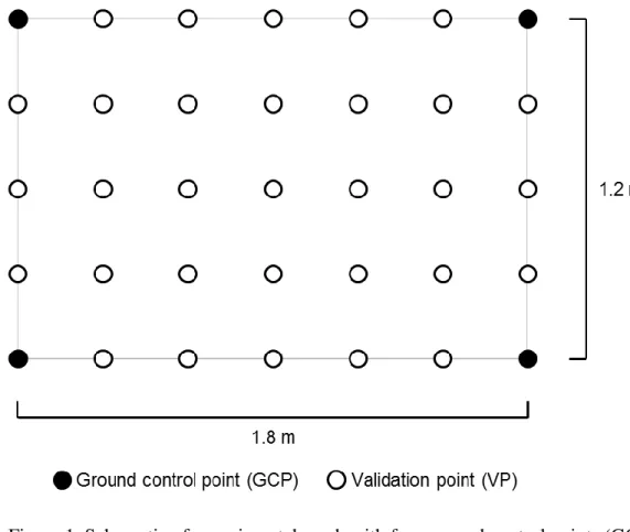
A simulated channel reach was established on a flat asphalt surface. This reach was intended to mimic the design of in-field ephemeral gully reaches. The reach was defined as the area within a 1.8 m by 1.2 m PVC frame, which was also utilized for the placement of anchor points that delineated channel reaches monitored in the field study (Wells et al., in prep.). Asphalt was chosen as the experimental surface because it was primarily flat and smooth yet still had modest texture on a gentle slope. Within the reach, 35 photogrammetric targets were placed in a 0.3 m grid (Figure 1). The targets were surveyed with a Trimble R8 real-time kinematic global positioning system (RTK-GPS) receiver, which has maximum horizontal and vertical accuracies of 0.8 cm and 1.5 cm,
respectively (Trimble Navigation Ltd., 2013). The receiver was connected to the Iowa Real-Time Network (IaRTN) maintained by the Iowa Department of Transportation, which is a network of base stations with a 1σ vertical accuracy of 2 to 3 cm (Iowa DOT, 2014). This RTK-GPS survey dataset was used as the reference dataset in the subsequent analyses. Of the 35 targets, the four that were located in the reach corners were used as ground control points (GCPs) for photogrammetric processing and the 31 remaining targets were used as validation points (VPs). The GCPs in this configuration correspond to field reaches defined by sets of four surveyed reference stakes placed sequentially along actual channels. The GCPs were used as vertices of a quadrilateral that defined the extents of the asphalt reach, which had an area of 2.11 m2.
The experimental reach was photographed with a non-metric pre-calibrated Nikon D7000 digital single-lens reflex camera containing an AF Nikkor lens with f/2.8D
aperture and fixed 20 mm focal length. Image files were saved in JPEG format. The camera was mounted on a metal frame attached to a backpack. The photographer then wore the backpack which resulted in a camera height of approximately 3.1 m. The camera was connected to a Cam Ranger wireless router that allowed the photographer to use an iPad to view the imaging area and capture photographs without touching the camera (Wells et al., in prep.).
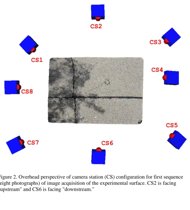
Two sequences of convergent oblique images were obtained, and every
photograph contained the entire reach. When oblique camera angles are used the size of a pixel in object space is dependent upon its location in image space (Heng at al., 2010), so camera location must be known or solvable. In this case, camera locations were
calibration parameters. Oblique photographs were used because images that converge on the scene improve the solution of camera orientation and thus also the accuracy of the reconstructed surface (Stojic et al., 1998; Eos Systems Inc., 2012). First, eight
photographs were taken in a circular fashion around the reach. Automatically resolved camera positions for the first sequence of images are shown in Figure 2. In field-based photography of channel reaches, one photograph is obtained from the downstream side facing upstream parallel to the channel and a second is taken from the upstream side of the reach facing downstream (Wells et al., in prep.). To mimic this procedure the second set of photographs included three images from the "downstream" side and three images from the "upstream" side of the experimental reach.
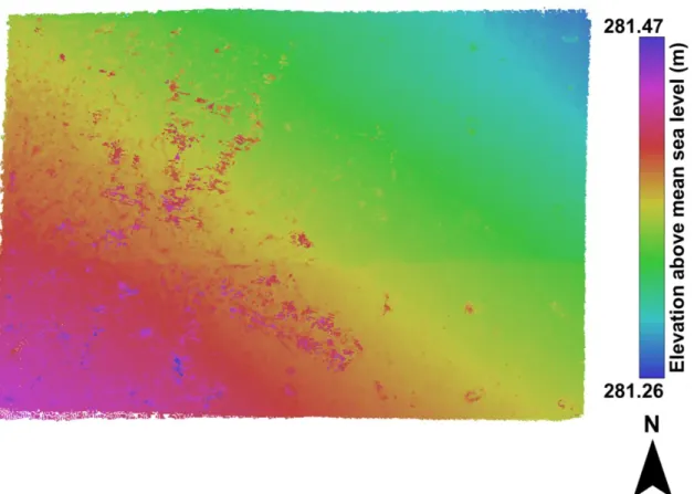
The eight photographs obtained in the first sequence were all used as input to generate a point cloud in PhotoModeler Scanner (Eos Systems Inc., 2014). To create the point cloud, first all eight images were matched with PhotoModeler Scanner's automated image matching procedure, which is based on the scale-invariant feature transform (SIFT) algorithm (Lowe, 2004). The four GCPs in every photograph were each manually identified and then cross-referenced to the corresponding GCP in each of the other images. The GCPs were then geo-referenced using the RTK-GPS survey data. Geo-referencing prior to point cloud generation is beneficial because it automatically scales and orients the point cloud as it is computed. Finally, the point cloud was generated using the Create Dense Surface command within PhotoModeler Scanner. All paired photos were used, sampling interval was set to 5 mm, and default meshing options were used. The resulting point cloud was exported as a text file (Figure 3).
The set of six additional photographs was used to generate nine point clouds with PhotoModeler Scanner. Each of the "upstream" facing photographs was matched with each of the "downstream" facing photographs for a total of nine image pairs. Every image pair was used as input to create a point cloud according to the procedure described above, with the only difference being that two photographs were used instead of eight. The image pairs and corresponding point clouds are shown in Figure 4. The resulting nine point clouds were exported as text files.
Comparison of replicated models of the same surface has been proposed (Heng et al., 2010; Wheaton et al., 2010) and used (Brasington and Smart, 2003) as an approach to assess DEM uncertainty. This tactic was adopted for the ensuing analysis. Each of the nine point clouds generated from the second image set was paired with every other point cloud for a total of 36 pairs. Wells et al. (in prep.) have developed a straightforward procedure that can be applied to determine the discrepancy, expressed as volumetric change, between the surfaces approximated by two point clouds. This is mathematically analogous to subtracting one surface from the other. In theory, any volume difference thus computed using the 36 point cloud pairs should equal 0 m3 because the nine point clouds represent the same surface. However, the errors inherent in any general case of surface reconstruction and in this specific application of close-range photogrammetry suggest that the inevitable inconsistencies between point clouds should result in a non-zero volume difference.
To verify this supposition, volumetric discrepancy, ΔV, between surfaces was calculated for all 36 point cloud pairs using the point cloud post-processing approach of Wells et al. (in prep.), which is briefly summarized here. Two input point cloud files p
and q are interpolated to a 5 mm raster grid containing i × j cells, each with elevation Zij.
The volume difference between the surfaces represented by p and q is given by
∆𝑉 = 𝑎 ∑ ∑(𝑍𝑞− 𝑍𝑝)
𝑗 𝑖
(1)
where a is the area of one raster cell (equal for all cells), i and j are indices corresponding to the location of an individual cell, and Zp and Zq are the interpolated elevations at cell ij
within the DEMs fitted from p and q, respectively.
When subtracting the replicate surfaces approximated by the nine point clouds, the minuend and subtrahend were determined with a random number generator. For each point cloud pair a 0 dictated that the point cloud represented by the alphabetically later letter would serve as the minuend (e.g. ΔVAB = B – A); a 1 indicated the opposite (e.g.
ΔVAB = A – B). The distribution of volumetric changes was assessed and summary
statistics were calculated using R statistical software (R Core Team, 2013). Two times the standard deviation (2σ) of the population of volume changes was taken as the
uncertainty in calculation of volume change, δΔV, as determined by the photogrammetric method employed in this study, where two standard deviations of a population with a Gaussian distribution approximates a 95% confidence level (Taylor, 1997). Normality of all populations was verified with the Shapiro-Wilk test.
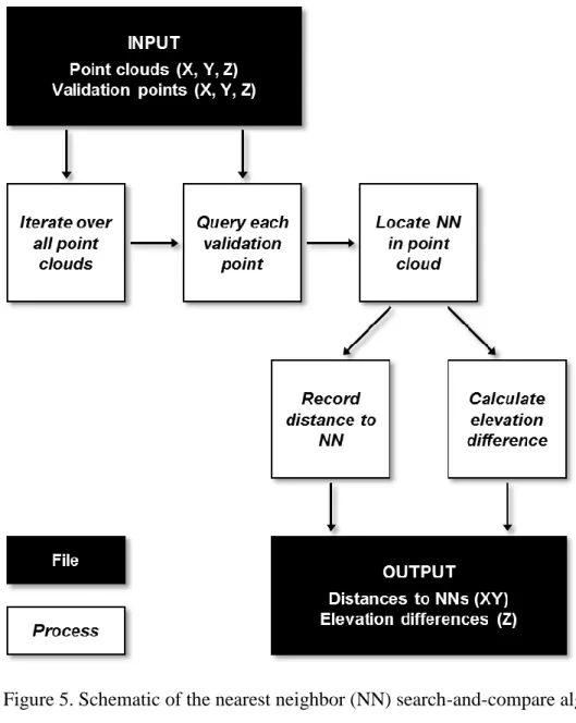
The quality of the elevation information contained in the point clouds was then assessed. For all nine point clouds the elevation of each of the 31 VPs was compared with the elevation of the closest point in the point cloud, which was determined with an in-house Python script. Raw point clouds rather than rasterized DEMs were used as input to preclude any interpolation errors. The program utilizes the NumPy library (Dubois et al., 1996; van der Walt et al., 2011) to rapidly organize and query point cloud geospatial data
for the nearest neighbor of every validation point. Once the nearest neighbor is located, the distance between the VP currently under consideration and its nearest neighbor along with the elevation difference between them are computed and recorded. Elevation
difference, 𝑍̂, is calculated by
𝑍̂ = 𝑍𝑁𝑁− 𝑍𝑉𝑃 (2)
where ZNN is the elevation value of the nearest neighbor within the point cloud and ZVP is
the elevation of the validation point against which the neighbor is being compared. The formulation of Equation 2 suggests that for any validation point VPi if the corresponding
elevation difference 𝑍̂i > 0 then the surface approximated by the point cloud
overestimates elevation relative to the surveyed VPi, which serves as the reference value.
The inputs, processes, and outputs of the nearest neighbor search-and-compare algorithm are summarized in Figure 5. The results of running the script with nine point clouds and 31 VPs were outputted as a text file and analyzed with R statistical software.
In determination of photogrammetric point cloud quality, the spatially averaged elevation difference was used to compute the relative vertical accuracy, δZrel, and the standard deviation of validation point-to-nearest neighbor elevation differences was understood to represent the absolute (geo-referenced) vertical accuracy, δZgeo-ref, of the point clouds. Uncertainty of elevation change, δΔZ, was defined as
𝛿∆𝑍 = 𝛿Δ𝑉 𝐴⁄ 𝑅 (3)
where AR is the area of the reach. This is analogous to average volume change per unit
area, or mean elevation difference across an entire surface model. Vertical change uncertainty was derived from volumetric change uncertainty because determination of volumetric change within channel reaches is one goal of the field study. Furthermore,
utilization of descriptive statistics from a population of volume differences to define the probable range of vertical change accounts for additional errors that may be introduced by interpolation and rasterization during point cloud post-processing. The use of volume change uncertainty to establish elevation change uncertainty is based on the assumption that vertical uncertainty is not spatially variable within the reach, that is for any
individual point cloud the error associated with elevation is uniform at all locations within that point cloud. The value calculated by Equation 3 is associated with uncertainty of change in elevation between DEMs. This value is actually a combination of the
vertical uncertainty of each surface in a pair. If the vertical errors of individual DEMs p and q are assumed to be independent and random, then they can be propagated into vertical change error, 𝜀Δ𝑍, using the sum in quadrature approach of Taylor (1997,
Equation 3.16) such that
𝜀Δ𝑍= √(𝛿𝑍𝑝)2+ (𝛿𝑍𝑞)2 (4)
where δZp and δZq are the vertical uncertainties associated with the surfaces
approximated by point clouds p and q, respectively, and 𝜀Δ𝑍is equivalent to δΔZ. If it is
assumed that the vertical uncertainties of individual surfaces p and q are equal such that δZp = δZq = δZrel then Equation 4 can be rearranged and simplified to yield
𝛿𝑍rel = 0.707𝜀∆𝑍 (5)
where δZrel is the vertical uncertainty of the surface described by any one point cloud. This value is useful as an indicator of vertical accuracy because it provides a measure of typical elevation discrepancy across the entire horizontal area described by a point cloud. Similarly, the volume change calculation in Equation 1 integrates elevation change over the entire raster grid area.
Two times the sample standard deviation (2σ), root mean square error (RMSE), and mean absolute error (MAE), were calculated as metrics of uncertainty for ΔV, δΔZ, δZrel, and δZgeo-ref with the following equations:
2𝜎 = 2√ 1 𝑁 − 1∑(𝜀𝑖 − 𝜀̅)2 (6) RMSE = √1 𝑁∑ 𝜀𝑖2 (7) MAE = 1 𝑁∑|𝜀𝑖| (8)
where N is a sample size; 𝜀𝑖 is an individual error of volume change, elevation change, or elevation; and 𝜀̅ is the mean error of an entire population of volume change, elevation change or elevation errors.
Results
The point cloud generated with the set of eight photographs contained 2,468,517 points within the reach area of 2.11 m2, which corresponded to a point density of 1.17 points mm-2. Point clouds A through I generated from the set of six images contained an average of 94,620 points inside the reach, or 0.045 points mm-2.
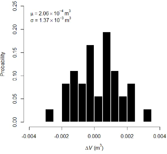
A histogram of the 36 computed volume differences is shown in Figure 6, and a Shapiro-Wilk test (W = 0.986, p = 0.9195) validated the graphical evidence of a Gaussian distribution. Mean volume difference was 2.06 × 10⁻⁴ m3 and the sample standard
deviation of volume differences was 1.37 × 10⁻³ m3. Thus δΔV within the experimental reach was defined as ± 2.73 × 10⁻³ m3. A one-sample t-test (t = 0.9047, df = 35, p = 0.3718) showed that the mean volumetric discrepancy was not significantly different
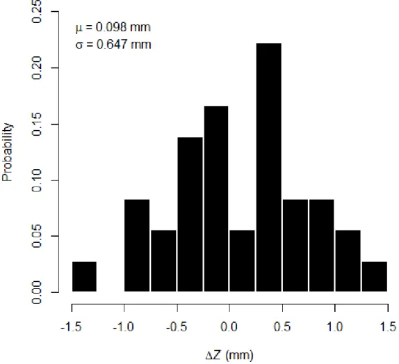
from zero. Based on this value of δΔV, the 2σ uncertainty of elevation change, δΔZ, was calculated as ± 1.29 mm with Equation 3. Inserting this value into Equation 5 yielded an individual point cloud 2σ relative vertical uncertainty, δZrel, of 0.916 mm. Figure 7 illustrates the distribution of spatially averaged elevation discrepancies (computed by dividing the population of volume differences by the reach area, as in Equation 3) which had an unbiased mean of 0.098 mm (one-sample t-test: t = 0.9047, df = 35, p = 0.3718) and a standard deviation of 0.647 mm with a normal distribution (Shapiro-Wilk test: W = 0.986, p = 0.9195).
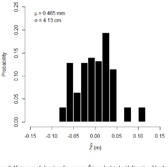
The results of the point cloud quality assessment via the nearest neighbor script are summarized in Figure 8. There was no significant correlation (r = 0.245) between validation point-to-nearest neighbor distance and elevation difference (Figure 9). Mean distance between validation points and their nearest neighbor was 3.09 mm (less than the width of one raster cell, 5 mm) and mean elevation difference was 0.465 mm, while the standard deviation of elevation differences was 4.13 cm. A Shapiro-Wilk test (W = 0.9681, p = 7.274 × 10⁻⁶) revealed that the population of elevation differences did not have a Gaussian distribution. Based on a one-sample t-test (t = 0.188, df = 278, p = 0.851), the mean elevation discrepancy of 0.465 mm was not statistically different from zero. Two times the standard deviation of elevation differences, 8.26 cm, was used as the 2σ geo-referenced absolute vertical accuracy, δZgeo-ref, of photogrammetric point clouds. Together with graphical evidence of normality (Figure 8), a non-parametric 95%
confidence interval of –7.39 to 11.06 cm suggests that the population of elevation differences is only approximately Gaussian because it is more heavily tailed and slightly positively skewed.
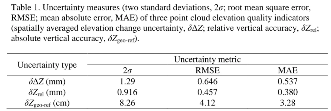
2σ values were assumed to be the preferred uncertainty metric due to the associated high level of confidence, although root mean square (RMS) error and MAE were also computed using Equations 6, 7, and 8, respectively, for δΔZ, δZrel, and δZgeo-ref. These results are compiled in Table 1.
Discussion
The point cloud generated using eight images contained approximately 26 times more points than the point clouds generated using paired photographs. While the point density of 0.045 points mm-2 of the two-image point clouds appears to be low, it is worth noting that, during post-processing, point clouds are interpolated to 5 mm grids, which means that a 0.045 points mm-2 density corresponds to 1.12 points per raster cell (25 mm2). This value suggests that interpolation-induced error should be small even when only two photographs are used because the number of points exceeds the number of raster cells. Such data redundancy typically increases DEM accuracy (Ackermann, 1996).
Because more photographs improve the accuracy of any photogrammetrically reconstructed surface (Eos Systems Inc., 2012; Fonstad et al., 2013), the validity of using only two images in lieu of eight was assessed by comparing point clouds A through I with the eight-image point cloud. The average ΔV was 2.77 × 10⁻³ m3 and the corresponding average vertical difference was 1.31 mm. Both of these values compare well with the δΔV and δΔZ values of ± 2.73 × 10⁻³ m3 and ± 1.29 mm, respectively, as calculated above. The primary benefit of using only two photographs is reduced time to generate a point cloud. Using the set of eight photographs as input in PhotoModeler Scanner, an experienced operator took almost two hours to create the final point cloud, including manual GCP identification and cross-referencing in addition to automated image
matching and dense surface calculation. The same operator was able to use the exact same procedure to create point clouds in approximately 15 minutes when using only pairs of images. Because the typical volumetric and vertical differences between the surface constructed from eight photographs and surfaces from photograph pairs were similar to the 95% probability intervals for both volume change and elevation change, the time-saving approach of using only two images per point cloud was accepted on the basis that image pairs can be used to reconstruct any experimental surface of interest with sufficient accuracy.
The uncertainty associated with volume change, δΔV, in the experimental reach was established as ± 2.73 × 10⁻³ m3 based on 2σ of the population of ΔV values, which corresponds to a 95% confidence level that true volume change values are within this range from observed values. There is no significant bias to this approach, as indicated by the fact that the mean ΔV of 2.06 × 10⁻⁴ m3 was not significantly different from zero. However, applying this volume change uncertainty to in-field ephemeral gully reaches is complicated by the fact that not every reach encompasses the exact same ground area. Thus, an uncertainty of volume change averaged per unit area, expressed as a range for elevation change (at 95% probability), is preferable. The uncertainty of vertical change, δΔZ, calculated as ± 1.29 mm implies a 95% probability that the discrepancy between any observed elevation change and the actual elevation change is within this amount from calculated values.
Using the δΔZ value of ± 1.29 mm along with Equations 4 and 5 resulted in a 2σ relative vertical point cloud accuracy, δZrel, of 0.916 mm. The calculation of this accuracy value assumes that errors in one point cloud are independent of errors in another point
cloud. Even though some comparisons involved point clouds with a common photo (e.g. point clouds E and H both used photograph KGA_0785 for photogrammetric image processing) the fact that every point cloud had at least one unique source photograph each time it was compared with other point clouds satisfied this assumption because image matching (i.e. the SIFT algorithm) depends on both photographs in a stereo pair. This value is twice as large as the elevation standard deviation (1σ) of any one point cloud relative either to itself or to another point cloud that exists in the same arbitrary (i.e. not geo-referenced) Euclidian three-dimensional space of real-world scale. The theoretically obtainable vertical accuracy of a DEM can be 1 × 10⁻⁴ of the object distance (Ackermann, 1996). Thus for a camera height of approximately 3.1 m a maximum vertical accuracy of 0.31 mm could be expected. Encouragingly, the 2σ vertical point cloud uncertainty, δZrel, of 0.916 mm approaches this theoretical optimum and is on the same order of magnitude. For a reconstructed surface model of this size, a maximum vertical RMS error of 1.664 mm can be expected (Eos Systems Inc., 2012). The δZrel value of 0.916 mm is within this upper limit, as is the RMS error of an individual point cloud of 0.457 mm.
The 2σ absolute vertical accuracy, δZgeo-ref, of photogrammetric point clouds as determined by comparison of validation points with their nearest neighbors was found to be 8.26 cm. This accuracy of elevation values is in an absolute sense, that is, the elevation of a point cloud with respect to a fixed vertical datum (mean sea level: the same datum of the RTK-GPS survey). Thus, there is 95% confidence that a geo-referenced point cloud – which is necessary for multi-temporal surface differencing of field-monitored channel reaches – generated by this technique is located within 8.26 cm of its true vertical location on the surface of the earth. Furthermore, the fact that the mean elevation
difference of 0.465 mm determined from the output of the nearest neighbor search-and-compare script is not significantly different from zero suggests that there is no positive or negative bias of mean point cloud elevation in real-world coordinates.
The GCPs used for geo-referencing during point cloud generation were surveyed along with the 31 validation points used to define absolute vertical accuracy. Therefore, as long as point cloud relative elevation accuracy is high (e.g. < 1 mm, as in this
instance), it is logical that the absolute vertical uncertainty of any geo-referenced point cloud approaches the vertical accuracy of the survey equipment used. The 2σδZgeo-ref value of 8.26 cm is comparable to the Trimble R8 receiver and IaRTN 2σ vertical accuracy of approximately 4 to 6 cm. Optimum RTK-GPS accuracy was deemed
plausible because the horizontal accuracy of the surveyed GCPs was better than 2 cm: the distances between surveyed GCP coordinates were within approximately 2 cm of the actual ground distances between GCPs on the experimental surface. RMS error is another common metric of vertical accuracy. The RMS error of the 279 validation point-to-nearest neighbor elevation differences was 4.12 cm, which also compares well with the vertical accuracy of the RTK-GPS system utilized. Thus, the accuracy of the survey equipment constrained the accuracy of geo-referenced point clouds generated with this photogrammetric approach.
Erroneous GCP information due to survey error could influence point cloud elevation. The effect of GCP measurement error on point clouds was quantified by re-generating point clouds A through I with altered GCP values, such that the GCP elevations were first increased by 10 cm and then decreased by 5 cm relative to the original survey data. It was assumed for this analysis that elevation error would be equal
for all GCPs. Each erroneous point cloud was compared to its original counterpart, which resulted in average elevation differences of 9.99 cm and –4.98 cm for the +10 cm and –5 cm cases, respectively. Thus, vertical error in GCP measurement directly impacts the elevation of all points within a point cloud.
Utilizing geo-referenced GCPs to scale and orient point clouds would not impact multi-temporal elevation change error δΔZ, provided that the same GCP coordinates are used to scale and orient each point cloud. However, if GCPs are re-surveyed between photography, any comparison of the resulting point clouds (based on different GCP surveys) must take into account the individual accuracies of each GCP survey. Therefore, it is recommended that GCPs be (re-)surveyed according to best practices and under optimum conditions so as to maximize their accuracy, thereby minimizing the potential error of comparing multi-temporal geo-referenced point clouds.
Choice of uncertainty metric depends on planned data use. As Table 1 indicates, there are clear differences between 2σ, RMS error, and MAE as indices of vertical
geospatial data quality, such that 2σ uncertainty is the largest (i.e. the most conservative). Because no significant positive or negative vertical biases were observed, RMS error was nearly equivalent to 1σ for δΔZ, δZrel, and δZgeo-ref. If elevation change uncertainty δΔZ is used as a probability interval along with volumetric estimates of morphological
development, MAE would result in the smallest range and 2σ in the largest. If vertical change uncertainty is used as a minimum detection threshold (e.g. Brasington et al., 2000; Brasington and Smart, 2003; Fuller et al., 2003; Lane et al., 2003; Heritage et al., 2009; Gessesse et al., 2010; Wheaton et al., 2010; Hugenholtz et al., 2013), choice of 2σ
would cause the most information loss whereas selection of RMS error or MAE as the threshold level of detectable geomorphic change would preserve more information.
Comparison of models generated from repeated topographic reconstructions of the same surface was utilized to establish DEM vertical uncertainty (Brasington and Smart, 2003; Heng et al., 2010; Wheaton et al., 2010) and comparison of geo-referenced point clouds against surveyed validation points was used to determine absolute accuracy of elevation data (similar to Fonstad et al., 2013). It is beneficial to use surface
differencing to define uncertainty both of elevation and of vertical change because doing so accounts for all sources of potential error (e.g. interpolation and rasterization) and not solely error induced during point cloud generation. The high δZrel of 0.916 mm would allow for accurate determination of three-dimensional parameters such as soil surface roughness and four-dimensional values such as volume change, whereas the δZgeo-ref of geo-referenced point clouds of 8.26 cm would allow for confident integration of point cloud geospatial data into pre-existing DEMs with lower elevation accuracy, such as those derived from aerial laser scanning or other remote sensing techniques.
For field application of this technique to study soil erosion, it is necessary that the average magnitude of observed elevation changes be larger than the vertical change uncertainty of ± 1.29 mm. However, this δΔZ value was determined using a surface with little relief (17 cm), whereas gullies have greater relief. The influence of relief on vertical change uncertainty was quantified by replicating the procedure used for the asphalt surface but with images of an actual gully reach. The reach encompassed an area of 2.16 m2 and had relief of 63 cm. Six photographs and four surveyed GCPs were used to generate nine point clouds, which were all compared to calculate the uncertainty in
average elevation change. The 2σ uncertainty of vertical change based on post-processing of the nine point clouds with 63 cm relief was determined to equal ± 2.55 mm. The vertical change uncertainty was larger for the point clouds that represented the gully reach, but the uncertainty increase (by a factor of 1.97) was less than the relief increase (by a factor of 3.71). Therefore, depending on relief, the uncertainty of elevation change ranges from ± 1.29 to ± 2.55 mm, and uncertainty may increase further when images of deeper channels are used. A pair of convergent oblique images that both contain an entire reach and its four surveyed GCPs is all that is necessary to accurately reconstruct a segment of a channel formed by concentrated overland flow. Applying the uncertainty of elevation change (volume change per unit area, δΔZ) to field-monitored channels would allow for a 95% estimate confidence interval to be reported along with morphometrically derived estimates of ephemeral gully erosion.
Conclusions
Statistical analysis of the results of comparing repeated topographic models of an experimental asphalt surface yielded an individual digital elevation model 2σ relative vertical accuracy of 0.916 mm and a 2σ uncertainty of detecting elevation change between two point clouds of ± 1.29 mm. Comparison of the replicate digital surface models with a set of surveyed validation points showed that geo-referenced point clouds created with this application of close-range photogrammetry had an unbiased 2σ absolute vertical accuracy of 8.26 cm. Close-range digital photogrammetry allowed for highly accurate reconstruction of the experimental surface. The relief-dependent vertical change uncertainty range of ± 1.29 to ± 2.55 mm may be extended to estimates of channel
erosion that are based on morphological change in reaches reconstructed with close-range photogrammetry.
References
Abd Aziz, S., B.L. Steward, A. Kaleita, and M. Karkee. 2012. Assessing the effects of DEM uncertainty on erosion rate estimation in an agricultural field. Trans. ASABE 55(3):785-798.
Ackermann, F. 1996. Techniques and strategies for DEM generation. In: C.W. Greve, editor, Digitial photogrammetry: An addendum to the manual of photogrammetry. American Society of Photogrammetry and Remote Sensing, Bethesda, MD. p. 135-141.
Aguilar, M.A., F.J. Aguilar, and J. Negreiros. 2009. Off-the-shelf laser scanning and close-range digital photogrammetry for measuring agricultural soils microrelief. Biosyst. Eng. 103(4):504-517.
Brasington, J., B.T. Rumsby, and R.A. McVey. 2000. Monitoring and modelling morphological change in a braided gravel-bed river using high resolution GPS-based survey. Earth Surf. Process. Landforms 25(9):973-990.
Brasington, J., and R.M.A. Smart. 2003. Close range digital photogrammetric analysis of experimental drainage basin evolution. Earth Surf. Process. Landforms 28(3):231-247.
Castillo, C., R. Pérez, M.R. James, J.N. Quinton, E.V. Taguas, and J.A. Gómez. 2012. Comparing the accuracy of several field methods for measuring gully erosion. Soil Sci. Soc. Am. J. 76(4):1319-1332.
Dubois, P.F., K. Hinsen, and J. Hugunin. 1996. Numerical Python. Comput. Phys. 10(3):262-267.
Eos Systems Inc. 2012. Quantifying the accuracy of dense surface modeling within PhotoModeler Scanner.
www.photomodeler.com/applications/documents/DSMAccuracy2012.pdf (accessed 26 July 2014).
Eos Systems Inc. 2014. PhotoModeler Scanner (64-bit). Eos Systems Inc., Vancouver, British Columbia.
Fonstad, M.A., J.T. Dietrich, B.C. Courville, J.L. Jensen, and P.E. Carbonneau. 2013. Topographic structure from motion: a new development in photogrammetric measurement. Earth Surf. Process. Landforms 38(4):421-430.