New MPLS Network Management Techniques
Based on Adaptive Learning
Tricha Anjali, Caterina Scoglio, and Jaudelice Cavalcante de Oliveira
, Member, IEEE
Abstract—The combined use of the differentiated services (DiffServ) and multiprotocol label switching (MPLS) technologies is envisioned to provide guaranteed quality of service (QoS) for multimedia traffic in IP networks, while effectively using network resources. These networks need to be managed adaptively to cope with the changing network conditions and provide satisfactory QoS. An efficient strategy is to map the traffic from different DiffServ classes of service on separate label switched paths (LSPs), which leads to distinct layers of MPLS networks corresponding to each DiffServ class. In this paper, three aspects of the management of such a layered MPLS network are discussed. In particular, an optimal technique for the setup of LSPs, capacity allocation of the LSPs and LSP routing are presented. The presented techniques are based on measurement of the network state to adapt the network configuration to changing traffic conditions.
Index Terms—Adaptive learning, differentiated services multi-protocol label switching (DiffServ/MPLS) networks, Kalman filter, Markov decision process, network measurement, stochastic com-parison theory.
I. INTRODUCTION
W
ITH the advancement in the Internet technology, the users are demanding quality of service (QoS) guaran-tees from the network infrastructure. Several new paradigms have been proposed and implemented in the Internet for that purpose. Prominent among these are differentiated services (DiffServ) and multiprotocol label switching (MPLS) technolo-gies. Combined use of these two technologies can allow the satisfaction of these QoS guarantees to the users. However, new techniques need to be designed to facilitate the interworking of DiffServ and MPLS, provide the QoS by efficiently using the network resources [1] and to adapt the network to variable and unpredictable traffic conditions.The premise of MPLS is to attach a short fixed-length label to the packets at the ingress router of the MPLS domain. These edge routers are called label edge routers (LERs), while routers capable of forwarding both MPLS and IP packets are called label switching routers (LSRs). The packets are then routed based on the assigned label rather than the original packet IP header. The label assignments are based on the forwarding
Manuscript received January 20, 2004; revised April 8, 2005. This work was supported by the National Science Foundation under Award 0219829. The work for this paper was performed while the authors were at the Broad-band and Wire-less Networking Laboratory, Georgia Institute of Technology, Atlanta.
T. Anjali is with the Illinois Institute of Technology, Chicago, IL 60616 USA (e-mail: tricha@ece.iit.edu).
C. Scoglio is with Kansas State University, Manhattan, KS 66502 USA (e-mail: caterina@ksu.edu).
J. C. de Oliveira is with Drexel University, Philadelphia, PA 19104 USA (e-mail: jau@ece.drexel.edu).
Digital Object Identifier 10.1109/TNN.2005.853428
equivalent class (FEC), where packets belonging to the same FEC are assigned the same label and traverse through the same path across the MPLS network. A path traversed by an FEC is called a label switched path (LSP). The label distribution protocol (LDP) and an extension to the resource reservation protocol (RSVP) are used to establish, maintain (refresh), and teardown LSPs [2]. One of the most attractive applications of MPLS is traffic engineering (TE), since LSPs can be considered as virtual traffic trunks that carry flow aggregates [3]. However, MPLS by itself cannot provide service differentiation, which brings up the need to complement it with another technology capable of providing such a feature: the DiffServ. By mapping the traffic from a given DiffServ class of service on a separate LSP, DiffServ-aware MPLS networks can meet engineering constraints specific to the given class on both shortest and nonshortest path. This TE strategy is called DiffServ-aware traffic engineering (DS-TE) [4]. In [5], the authors suggest how DiffServ behavior aggregates (BAs) can be mapped onto LSPs. More details on MPLS and DiffServ can be found in [2] and [6].
Efficient provisioning of QoS in a network requires adaptive management of network resources. In an MPLS network, LSPs are the basic entities for adaptation. In particular, LSPs should be able to be: 1) added or deleted; 2) dimensioned; and 3) routed based on the measured network state. A simple LSP setup policy based on the traffic-driven approach has been proposed in [7], in which an LSP is established whenever the number of bytes forwarded within one minute exceeds a threshold. This policy reduces the number of LSPs in the network; however, it has very high signaling costs and needs high control efforts for variable and bursty traffic as in the case of a fully connected network. In [8], we have suggested a threshold-based policy for LSP setup. In [9], we have proposed an optimal version of that technique. It provides an online design for MPLS network depending on the current traffic load. The proposed policy is a traffic-driven approach and balances the signaling and switching costs. By in-creasing the number of LSPs in a network, the signaling costs increase while the switching costs decrease. In the policy, LSPs are setup or torn-down depending on the actual traffic demand. Furthermore, since a given traffic load may change depending on time, the policy also performs filtering in order to avoid os-cillations which may occur in case of variable traffic.
A simple LSP capacity allocation scheme is based on pro-visioning a bandwidth cushion. In [10] and [11], the cushion scheme has been applied for capacity allocation to flow aggre-gates in a physical link. Also some other prediction schemes based on Gaussian [12], [13] as well as local maximum [14] predictor can be used. However, these schemes are wasteful of
resources and not efficient. Our technique [15] reduces band-width wastage without introducing per-flow modifications in the resource reservation. The scheme is designed to be simple, yet effective. The first step of the scheme is to perform an optimal estimate of the amount of traffic utilizing the LSP based on a measurement of the instantaneous traffic load. This estimate is then used to forecast the traffic bandwidth requests so that re-sources can be provisioned on the LSP to satisfy the QoS of the requests. The estimation is performed by the use of Kalman filter [16] theory while the forecast procedure is based on de-riving the transient probabilities of the possible system states.
Currently adopted LSP routing schemes, such as OSPF and IS-IS, have the number of hops as the only metric used for routing calculations, which is not enough for QoS routing pur-poses. In order to introduce QoS requirements in the routing process, the widest-path (WSP) [17] and the shortest-widest path (SWP) [18] algorithms were designed. Modifica-tions to these routing algorithms have been proposed in order to reduce complexity, such as the shortest path, WSP, etc., which consider only path options in their decisions [19]. In [20], the authors discuss two cost components of QoS routing: complexity and increased routing protocol overhead. Improve-ments are suggested in order to reduce these cost components, such as path precomputation and nonpruning triggering policies. Some of these suggestions were used in our routing algorithm. Finally, another QoS routing algorithm called minimum inter-ference routing algorithm (MIRA) is presented in [21]. MIRA tries to minimize the interference between different routes in a network for a specific set of ingress-egress nodes. The short-comings of MIRA include its computation burden, the fact that it uses longer paths than shortest-path routing schemes, it is not able to estimate the interference effects on clusters of nodes, and it is not very likely to be implemented by vendors because of its complexity. The basic idea behind our technique [22] is to choose a routing scheme that performs the best among a set of routing schemes in a simulation of the traffic scenario obtained by measurement of the network state.
To illustrate the interrelations of the three techniques for LSP setup, capacity allocation and routing in MPLS networks, con-sider the scenario where the network planning phase has pro-vided an initial topology of the MPLS network that needs to be adapted to the changing traffic demands. Possible events could be the arrival of a bandwidth request or the arrival of a request for LSP setup based on SLS agreements. The arrival of a band-width request triggers the LSP setup technique which will de-cide whether to route the request on a pre-existing LSP path or to create a new LSP. In the latter case, the path for the new LSP needs to be found based on the current network state, and this path is obtained using the third technique presented in the fol-lowing. Initially, the new LSP is created based on the nominal value of the bandwidth requests but the actual allocation to the LSP should be adjusted based on the current traffic on the LSP. The second technique of LSP capacity allocation will be period-ically triggered to evaluate the utilization of the LSP and adjust the capacity, if required. In the case of arrival of a request for LSP setup, the routing and the capacity allocation techniques will come into play as explained before. Throughout this paper, we assume that the arriving bandwidth requests are an
aggrega-tion of individual flows and based on the Service Level Agree-ment, they are characterized by a constant and known bit rate.
These individual techniques are a part of an automated network manager called traffic engineering automated manager (TEAM) tool. TEAM is developed as a centralized authority for managing a DiffServ/MPLS domain and is responsible for dynamic bandwidth and route management. Based on the network states, TEAM takes the appropriate decisions and reconfigures the network accordingly. TEAM is designed to provide a novel and unique architecture capable of managing large scale MPLS/DiffServ domains. Details about the design and implementation of TEAM can be found in [23].
In this paper we present the theoretical framework used to de-velop the previous three techniques based on adaptive learning. In the case of LSP setup, we use the powerful theory of Markov decision processes. We model the system as Markovian band-width requests which trigger the decision of whether to setup or redimension an LSP. The requests arrive according to a Poisson process with rate and the request durations are exponentially distributed with rate . With the arrival of each request, the op-timal policy calculates the expected infinite horizon discounted total cost for provisioning the request by various methods and chooses the method with the lowest cost. This is a simple con-trol theoretic structure that is based on knowledge of the current network state. In the case of LSP capacity allocation, we use the well-known Kalman filter to obtain an optimal estimate of the number of active connections. The system model contains es-tablished connections out of which only some are active at any given instant of time. Based on a noisy measurement of the LSP traffic, we obtain an estimate of the number of connections uti-lizing the LSP and determine the bandwidth to be reserved for the LSP. In the case of LSP routing technique, we use the Sto-chastic Comparison theory. The system model contains a set of LSP routing schemes which are compared for their performance on a simulated scenario of previous LSP setup requests. The al-gorithm is able to determine the optimal LSP routing scheme among the set by comparing the LSP setup rejection probabili-ties of the various schemes, which is assumed to be more robust than the evaluation of the cardinal values of the rejection proba-bilities. In essence, this paper presents the synergistic operation of the three adaptive learning techniques for coordinated man-agement of the MPLS network. The contributions of this paper can be summarized as the following:
• present the three techniques for adaptive learning based MPLS network management;
• present the synergistic operation of the three techniques, • present numerical simulations illustrating the
perfor-mance of the three techniques.
The presented techniques learn the state of the network by real-time measurements and adapt the management policy for the network based on this learned state. This learning allows appro-priate decisions for providing the desired QoS in the network. The presented techniques fit the domain of adaptive learning in this sense.
This paper is structured as follows. In the next three sec-tions, we present the details of the individual adaptive learning techniques for MPLS network management. In Section II, we
present the LSP setup algorithm, which is followed by the LSP capacity allocation algorithm in Section III. In Section IV, we detail the LSP routing algorithm and in Section V, the integrated TEAM architecture for the network management is shown. In Section VI, performance of the presented techniques is evalu-ated and Section VII concludes the paper.
II. MDP-BASEDOPTIMALLSP SETUPALGORITHM
When a bandwidth request arrives between two nodes in a network that are not connected by a direct LSP, the decision about whether to establish such an LSP arises. In this section, we will first describe the model formulation and then obtain a decision policy which governs the decisions at each instant.
A. Model Formulation
We now describe the system under consideration. Let denote a physical IP network with a set of routers and a set of physical links . We define the following
notation for :
• : physical link between routers and ; • for : total link capacity of ; • for : number of hops between nodes and
.
We introduce a virtual “induced” MPLS network , as in [3], for the physical network . This virtual MPLS network consists of the same set of routers as the physical network and a set of LSPs, denoted by . We assume that each link of the physical network corre-sponds to a default LSP in which is nonremovable. The other elements of are the LSPs (virtual links) built between nonadja-cent nodes of and routed over s. Note that is a directed graph and . In other words, the different MPLS networks (for different class-types) are built by adding virtual LSPs to the physical topology when needed. In this paper, we will use the terms graph, network and topology interchangeably for the physical and MPLS networks and , respectively.
We define the following notation for .
• LSP : LSP between routers and (when they are not physically connected).
• LSP : default LSP between routers and (when they are physically connected).
• for : total capacity of LSP ( LSP not established).
• for : available capacity on LSP
( fully occupied).
• for : total bandwidth reserved between routers and . It represents the total traffic between router
as the source and router as the destination.
We assume that all LSP for have large capacity and this capacity is available to be borrowed by the other mul-tihop LSPs that will be routed over the corresponding physical links . We introduce a simple algorithm for routing LSPs on and bandwidth requests on . Each LSP must be routed on a shortest path in . We assume that
Fig. 1. MPLS network topology.
the shortest path between a source node and destina-tion node is the minimum hop path in and is de-noted by
In the MPLS network, the bandwidth requests between and are routed either on the direct LSP or on , which is a multiple-LSP path overlaying
LSP LSP
We also assume that is sufficiently large for all and whenever any LSP is redimensioned, it can borrow band-width from the physical links that it passes through.
The default and nondefault LSPs can be explained with the help of Fig. 1. The dotted lines between nodes 1–4, 4–6, and 6–8 represent the default-LSPs and the thick line between nodes 1–8 represents the direct LSP which is routed over the default-LSPs. With the assumed routing algorithm, we can define the fol-lowing two quantities.
• for : part of that is routed over
LSP .
• for : part of that is routed over
.
Note that is the total of the
band-width requests between and
is the total capacity of LSP and 0 for de-fault-LSPs since coincides with the LSP .
Let be the set of all LSP such that the corre-sponding shortest path contains the link . The following condition must be satisfied:
LSP
(1)
where 1 is a maximum fraction of that can be assigned to LSPs. Condition (1) means that the sum of capacity of all LSPs using a particular physical link on their path must not exceed a portion of the capacity of that physical link.
Definition 1: Decision Instants and Bandwidth Requests: We denote by the arrival instant of a new bandwidth request between routers and for the amount . The instant is called adecision instantbecause a decision has to be made to accommodate the arrival of the new bandwidth request.
We now describe the events that imply a decision. When a new bandwidth request arrives in the MPLS network at
instant , the existence of a direct LSP between and is checked initially. For direct LSP between and , the avail-able capacity is then compared with the request . If , then the requested bandwidth is allocated on that LSP and the available capacity is reduced accordingly. Otherwise, can be increased subject to condition (1) in order to satisfy the bandwidth request.
On the other hand, if there exists no direct LSP between and , then we need to decide whether to setup a new LSP and determine its corresponding . Each time a new LSP is setup or redimensioned, the previously granted bandwidth re-quests between and routed on are rerouted on the di-rect LSP . However, this rerouting operation is only virtual, since by our routing assumptions, both LSP and are routed on the physical network over the same .
Let be the departure instant of a request for bandwidth allocation routed on LSP . In this instant, we need to decide whether or not to redimension LSP , i.e., reduce its capacity .
We assume that the events and costs associated with any given node pair and are independent of any other node pair. This assumption is based on the fact that the new bandwidth requests are routed either on the direct LSP between the source and des-tination or on , i.e., the other LSPs are not utilized for routing the new request. This assumption allows us to carry the analysis for any node pair and be guaranteed that it will be true for all other pairs. Under this assumption, we can drop the ex-plicit dependence of the notations. Also we assume that nodes and are not physically connected. For the default LSPs, there is a large amount of available bandwidth and they too borrow bandwidth, in large amounts, from the physical links, if needed.
Definition 2: Set of Events: For each router pair and in the MPLS network, is theeventobserved at :
• 1 if there is an arrival of a bandwidth request for amount ;
• 0 if there is a departure of a request of amount
from ;
• 2 if there is a departure of a request from .
Definition 3: Set of States: For each router pair and in the MPLS network, we observe the system state when any event occurs. The state vector at a given time-instant
is defined as
(2) where is the available capacity on LSP is the part of that is routed over LSP and is the part of routed on . Note that the state–space , the set of all system states, is finite since is limited by which is in turn limited by the minimum of the link bandwidths on . is limited by and by minimum of default LSP bandwidths on . Also note that states with nonzero and are possible because just before the instant of observation, some user request might have departed leaving available bandwidth in LSP . The state information for each LSP is stored in the first router of the LSP.
Definition 4: Set of Extended States: The state–space of the system can be extended by the coupling of the current state and the event
(3) The set of extended states is the basis for determining the decisions to be taken to handle the events.
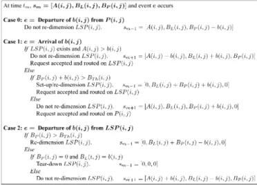
Definition 5: Set of Actions: The decision of setting up or redimensioning LSP when the event occurs, is captured by the binary action variable .
• 1 means that LSP will be setup or redimen-sioned and the new value of its capacity is set as
, where is considered negative if the event is a departure, either over LSP or .
• 0 means that no action will be taken on the capacity of LSP .
Definition 6: Decision Rules and Policies: A decision rule provides an action selection in each state at a given decision instant and a policy specifies the decision rules to be used
in each decision instant, i.e., .
If and , then the policy is stationary as the decision is independent of the time-instant. For most of the possible system states, the decision rule can choose an action from the set but there are a few states where only one action is possible. Those states and corresponding actions are the following.
• where 0 (the new
request is routed on LSP )
• 0 (the request ending
over )
• where 1 (LSP
is torn down)
Definition 7: Cost Function: The incremental cost
for the system in state , occurrence of the event , and the taken action is
(4) where is the cost for signaling the setup or redi-mensioning of the LSP to the involved routers, is the cost for the carried bandwidth and is the cost for switching of the traffic. The cost components depend on the system state and the action taken for an event.
The signaling cost is incurred instantaneously only when action 1 is chosen for state . It accounts for the signaling involved in the process of setup or redimensioning of the LSP. We consider that this cost depends linearly on the number of hops in over which the LSP is routed, plus a constant component to take into account the notification of the new capacity of the LSP to the network
(5) where is the coefficient for signaling cost per hop and is the fixed notification cost coefficient. This cost is not incurred
The other two components of (4) relate to the bandwidth and switching cost rates, respectively.
where is the sojourn time till the next event, i.e., until the system stays in state .
We assume that the bandwidth cost rate to reserve capacity units depends linearly on and on the number of hops in the physical shortest path over which the request is routed
(6) where is the bandwidth cost coefficient per capacity unit (c.u.) per time. Note that, from our routing assumption, the physical path is the same for LSP and for and, thus, the band-width cost rate depends only on the total carried bandband-width, ir-respective of the fractions carried over different paths.
The switching cost rate depends linearly on the number of switching operations in IP or MPLS mode and the switched bandwidth. The total number of switching operations is always since the physical path is fixed. Whether these switching operations are IP or MPLS depends on the path chosen in the MPLS network. For c.u. routed on LSP , we have 1 router performing IP switching and routers performing MPLS switching. For c.u. routed on , we have routers perform IP switching
(7) where and are the switching cost coefficients per c.u. per time in IP and MPLS mode, respectively. Summarizing, the signaling cost is incurred only at decision instants when 1, while the bandwidth and switching costs are accumulated con-tinuously until a new event occurs.
B. Optimal LSP Setup Policy
We propose a stochastic model to determine the optimal deci-sion policy for LSP setup. The optimization problem is formu-lated as a continuous-time Markov decision process (CTMDP) [24]. The cost functions for the MDP theory have been defined in Definition 7. Following the theory of MDPs, we define the ex-pected infinite-horizon discounted total cost, , with dis-counting rate , given that the process occupies state at the first decision instant and the decision policy is by
(8) where represent the times of successive instants when events occur and represents the fixed part of the
cost incurred whereas represents the
continuous part of the cost between times and .
Theoptimization objectiveis to find a policy such that:
The optimal decision policy can be found by solving the optimality equations for each initial state . We assume that the bandwidth requests arrive according to a Poisson process with rate and the request durations are exponentially dis-tributed with rate . With our assumptions of a discounted infinite-horizon CTMDP, the optimality equations can be written as
(9) where be the expected discounted cost between two de-cision instants and is the probability that the system occupies state at the subsequent decision instant, given that the system is in state at the earlier decision instant and action
is chosen. From (4), can be written as
(10) where represents the expectation with respect to the request duration distribution and represents the time before the next event occurs.
With the Markovian assumption on request arrival and du-ration, the time between any two successive events (arrival of requests or departure of a request) is exponentially distributed with rate . Recalling that between two successive events, the state of the system does not change, (10) can be rewritten as follows:
(11) (12) Since the set of possible actions is finite and is bounded, it can be proved that the optimal policy is sta-tionary and deterministic [24].
The solutions of the optimality equations give the optimal values of expected infinite-horizon dis-counted total costs. From one optimality equation, we derive that for the state where , the action would be (13), shown at the bottom of the next page and for state , the action would be (14), shown at the bottom of the next page.
This policy will be optimal if the thresholds are monotone nonincreasing which is true and can be proved through induction [24] by utilizing the linearity characteristics of the cost func-tions. These decisions have a control-limit structure. The values of can be found by using either value iteration or policy iteration algorithms.
Optimal LSP Setup Policy: The optimal policy
is stationary implying same decision rule at each decision instant and the decision rule is given by
for for
(15)
where and are given by
(13) and (14), respectively.
The threshold structure of the optimal policy facilitates the so-lution of the optimality equations but still it is difficult to precal-culate and store the solution because of the large number of pos-sible system states. So, we propose a suboptimal policy, called the least one-step cost policy, that is easy and fast to calculate.
C. Suboptimal Decision Policy for LSP Setup
The proposed least one-step cost policy is an approximation to the solution of the optimality equations. It minimizes the cost incurred between two decision instants. Instead of going through all the iterations of the value iteration algorithm, if we perform the first iteration with the assumption that 0, we obtain the third equation shown at the bottom of the page. From these single-step cost formulations, we can derive the action decision. For the state
, we obtain
otherwise for (16)
upon comparison of the two terms of . Sim-ilarly, comparing the two terms of , we get the action decision
otherwise (17) In both (16) and (17),
(18) By calculating for all , we minimize one-step cost of the infinite-horizon model. Since in the value itera-tion algorithm converges to the one-step value is a significant part of . The value of is very easy to calculate.
Least One-Step Cost LSP Setup Policy: The one-step optimal policy # # # # is stationary implying same de-cision rule at each dede-cision instant and the dede-cision rule is given by
# for
for (19)
where and are given by
(16) and (17), respectively.
The algorithm given in Fig. 2 can be implemented for our threshold-based suboptimal least one-step cost policy for LSP setup/redimensioning.
otherwise (13)
otherwise (14)
for
Fig. 2. Setup/redimensioning policy.
As can be seen in Fig. 2, the capacity of a new LSP is set equal to the sum of the nominal values of the individual bandwidth requests and is kept constant till the next redimensioning, as given in Fig. 2. However, this capacity may not be fully utilized all the time because of the variation in the profile of the current traffic flows. So, the second technique of capacity allocation is triggered for a better resource utilization.
III. KALMANFILTERBASEDLSP CAPACITYALLOCATION
There exists an LSP LSP between two routers. We estimate the level of traffic on this LSP, for a given traffic class, based on a periodic measurement of the aggregate traffic on LSP . In the following, we remove the explicit indexes in the notation for clarity, since we are concentrating on one node pair. We assume that the traffic measurements are performed at discrete time-points for a given value of . The value of is a measure of the granularity of the es-timation process and denotes the renegotiation instants. Larger values imply less frequent estimation which can result in larger estimation errors. We assume periodic renegotiation instants like other approaches. At the time instant (corresponding to ), the aggregate traffic on the LSP for a given traffic class is denoted by . We also assume that for the duration , the number of established sessions that use the LSP is . For each session, flows are defined as the active periods. So, each session has a sequence of flows separated by periods of inactivity. For a given traffic class, we denote by the number of flows at the instant and by
the number of flows in the time interval , without notational conflict. Clearly, and is not known/measurable. We assume that each flow within the traffic class has a constant rate of bits per second. So, nominally, for a traffic class
(20) As far as the measurement noise is concerned, for security and privacy reasons, information in the routers cannot always be ac-cessed. This is why a large effort in the scientific community has been devoted to the design of methods for the measurement of
available bandwidth [25]–[27]. Available bandwidth is comple-mentary to the utilization, so measuring available bandwidth is equivalent to measuring the aggregate traffic on the link. How-ever, these methods are active measurements and, thus, intrinsi-cally not exact. They are based on the transmission of packets at increasing speeds, up to a maximum which is taken as the value of the available bandwidth. This is the main basis for the belief that traffic measurements are noisy and a filter has to be used to estimate the real value of the aggregate traffic. However, even in the case in which router information can be accessed, the use of a tool to retrieve the information from the routers is still required. One of the most popular tools is multirouter traffic grapher (MRTG) [28], which we have used for obtaining the real data in our performance evaluation section. Compared with the previous methods based on active measurement, MRTG pro-vides more accurate measurements but still delays and errors in the transfer of the information can occur. To maintain the gen-erality of the measurement noise, we assume that this noise is characterized as a zero-mean Gaussian white noise process.
We concentrate, without loss of generality, on a single traffic class and its associated resource utilization forecasting. To con-sider a scenario with different classes of traffic with different bandwidth requirements, the same analysis can be extended and applied for each class. In this paper, we deal with the resource allocation for the DiffServ expedited forwarding (EF) classes, for which the assumption of constant resource requirement is valid. The underlying model for the flows is assumed to be Poisson with exponentially distributed interarrival times (pa-rameter ) and durations (parameter ). Characteristics of IP traffic at packet level are notoriously complex (self-similar). However, this complexity derives from much simpler flow level characteristics. When the user population is large, and each user contributes a small portion of the overall traffic, independence naturally leads to a Poisson arrival process for flows [29], [30]. The following analysis has been carried out using this assump-tion and then the numerical simulaassump-tions show that the capacity forecast is very close to the actual traffic.
Our scheme for resource allocation is split into two steps. In the first step, a rough measure of the aggregate traffic is taken and it is used to evaluate the number of flows through the Kalman filter estimation process. The Kalman filter imple-ments a predictor-corrector type estimator that is optimal in the sense that it minimizes the estimated error covariance. The es-timation error in this step is accounted for in the second step where we reserve the resources on the LSP for the time based on the forecast of the evolution of . This allocation is performed by choosing a state greater than the current utilization estimate such that the transition prob-ability to the state is low. This approach provides an upper en-velop for the estimate provided by the first step. It handles the errors caused by underestimation which can have a negative im-pact on the QoS.
A. Traffic Estimation
The only measurable variable in the system is which is a measure, corrupted by noise, of the aggregate traffic on the LSP. Nominally, , but we do not have access to the correct measurements of , even though is a known
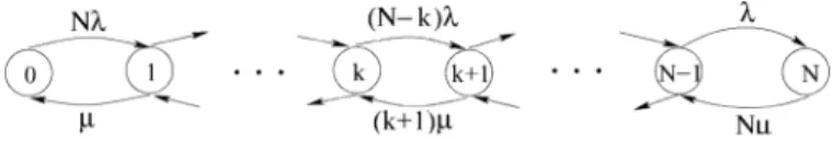
Fig. 3. State-transition-rate diagram.
quantity for a particular traffic class. Thus, we propose to use the Kalman filter setup to evaluate , an estimate of the actual , using the noisy measurements. Real mea-surement noise makes noisy. In other words, the measure-ments obtained from the network for the instantaneous traffic on the link can be noisy due to miscalculation, misalignment of timings etc. To use the Kalman filter setup, we need to find a
relation between and , and and . To
this purpose, we define to be the
probability that the number of active flows at time is , i.e., for
(21) The state-transition-rate diagram is shown in Fig. 3. The dia-gram depicts transitions among the states. From the diadia-gram and by using queuing theory [31], we can write the following differ-ential equations (22)–(24) for the probabilities :
(22)
(23) (24) The generating function is defined as the z-transform of the probability distribution function. It aids in the computation of the mean and variance of the probability distribution. Next, we calculate using (22)–(24) as
Utilizing the initial condition , i.e., the number of active flows at time is , we arrive at the following solution for : for
where
By the definition of the generating function and the special prop-erties of the z-transform, we get
(25) Thus, from the Kalman filter setup, we get
(26) where is Kalman filter gain and
This gives an estimate of the traffic on the LSP currently. This estimate will be used to forecast the traffic for the purpose of resource reservation.
B. Bandwidth Request Forecasting
The optimal estimate of the number of active flows can now be used to forecast , the resource requirement on
the LSP . To this purpose, for , we
define
(27) same as (21) in Section III-A. We also define and as shown in the equation at the bottom of the page, from (22)–(24). It can be seen that . It is easy to demonstrate that is similar to a real symmetric matrix and reducible to a diagonal form
where is a diagonal matrix with eigenvalues of and is the matrix of corresponding right eigenvectors . The
.. .
..
eigenvalues can be found to be for
which proves that is nonpositive definite, guaranteeing the existence of a solution for . The solution, for
, is given by
(28) where is a constant vector determined from the initial condi-tion ( at instant ) as
(29) where is a vector with all 0’s except the th element which is 1. Also we define
(30) using the notation that integral of a matrix is the integral of each element of the matrix. The elements of the vector denote the probabilities of transitioning to state at instant . Now we define as
(31) In words, we determine the minimum greater than or equal to such that the probability to be in state during the in-terval is less than a given threshold , in ef-fect choosing a state greater than the current utilization estimate such that the transition probability to the state is low. Then the resource requirement is forecasted to be
(32)
IV. STOCHASTICCOMPARISONBASEDLSP ROUTING
In this section, a formulation of the LSP routing problem is presented, including explanations on how to use SPeCRA for its solution.
Assume an LSP routing scheme (e.g., shortest-path) is denoted by . A set of possible LSP routing schemes (e.g., shortest-path, K-shortest-path, shortest-widest-path, etc.) will be denoted by . We will consider the percentage of rejected LSP setup requests in an interval to be an estimate of the probability of LSP setup rejection. This percentage depends on the LSP routing scheme adopted and also on the particular realization of the stochastic process characterizing the traffic. In conclusion, the percentage of rejected LSP setup requests from time 0 to can be denoted by the function .
If the traffic stochastic process is ergodic, the percentage of rejected LSP setup requests in the interval reaches the steady-state value. This value does not depend any longer on the particular realization, but only on the routing scheme , and represents the LSP setup rejection probability of the network at steady state, with routing scheme .
Suppose the stochastic process representing the traffic is sta-tionary and let be the fraction of rejected LSP setup requests in the interval , with the LSP routing scheme and with the stochastic process realization ; then with probability
1, the limit exists and represents
the LSP setup rejection probability of the network at the steady state. The LSP setup rejection probability is the objective function to be minimized. In the stationary scenario, the opti-mization problem is that of finding .
If the stochastic process characterizing the traffic is nonsta-tionary, which is the case of interest in this paper, the previous argument can be extended to the case of “piecewise stationary” traffic: i.e., If there exists a set of time instants, which we callswitching times, the stochastic process charac-terizing the traffic is stationary in every time interval
( th steady interval), and it becomes nonstationary at every switching time. In the following, we will assume that the steady intervals are long enough that the network can be considered at steady state for a large fraction of them.
With reference to piecewise-stationary traffic, we want to de-sign an algorithm which is able to determine, in every steady interval, the optimal LSP routing scheme in . We will call the optimal LSP routing scheme at time , which leads to the minimal LSP setup rejection probability at the steady state if the system remains stationary after the time , i.e.,
. Our objective is that of finding, at every time instant, the optimal .
Consider now a short time interval , which is con-tained in a steady interval (namely, there exists an such that , during which no change is made in the LSP routing scheme. An estimate of is given by the fraction of LSP setup requests rejected in such an interval:
.
If we change the LSP routing scheme into , we can verify
that, in general, . Under
very conservative assumptions, it is possible to prove [32] that the estimate of the order between and in terms of LSP setup rejection probability, is more robust than the estimate of the car-dinal values of the two LSP setup rejection probabilities. In fact, if there are independent estimates of and
taken on different and nonoverlapping intervals, the conver-gence rate of the estimated order to the real order is an expo-nential function of and is much larger than the convergence rate of the cardinal estimates, whose variance approaches 0 with . Such an interesting feature is used in SPeCRA, where we assume that the piecewise stationary characterizations of the traffic are denoted by , with .
Summarizing, we have a discrete and finite set of stationary stochastic processes, from which we can compose a nonstationary traffic by selecting any combination of s (A nonstationary traffic composed by several s is shown in Fig. 4). For each element , there exists a routing scheme which is optimal, within a set of possible routing schemes (routing scheme leads to the minimum rejection rate ). We do not know a priori which is the current , neither where the switching times among the s are located. SPeCRA should be able to
Fig. 4. Nonstationary traffic profile.
determine the optimal without knowing which is the current traffic offered to the network. The details of SPeCRA are described next.
A. Stochastic Performance Comparison Routing Algorithm
In order to explain SPeCRAs implementation, we define an increasing sequence of time instants , and denote the interval as the th control interval.
The algorithm always behaves as a homogeneous Markov chain and the optimal routing scheme is a state of the chain which is visited at the steady state with a certain probability. Aiming to reduce the chance that we could leave the state due to estimation error, we introduce a filter that reduces the effect of such estimate errors. The presence of this filter removes possible oscillations in the decision about the route selection. Changes are less likely to happen if the adopted routing scheme (state) is “good.” This is achieved by introducing a state variable (see the step 3 of the iteration in the following algorithm), which re-duces the change from “good” to “bad” routing schemes, while does not reduce the change from “bad” to “good.” The algorithm is detailed in the following.
• Data:
— The set of possible routing schemes .
— The probability function , which represents the probability of choosing as candidate routing scheme when the current routing scheme is .
— An initial routing scheme . — A time duration .
• Initialization:Set 0, and 0. • Iteration :
1) Let be the current routing scheme and choose
a set of candidate routing
schemes, where the selection of is made according
to .
2) Record all the LSP setup requests arrived and ended during the interval : Compute , the es-timates of the LSP setup rejection
probabili-ties for each routing scheme . Select .
3) Choose a new routing scheme according to the estimates computed in the previous step: let
and be
the estimates of the LSP setup rejection probabilities and for the two schemes and , respectively, in the th control interval.
If
0 else
4) Set and go to step 1.
V. TEAM: THEINTEGRATEDARCHITECTURE
The previous techniques are a part of TEAM along with other methods for LSP preemption and network measurement. TEAM is developed as a centralized authority for managing a Diff-Serv/MPLS domain and is responsible for dynamic bandwidth and route management. Based on the network states, TEAM takes the appropriate decisions and reconfigures the network ac-cordingly. TEAM is designed to provide a novel and unique ar-chitecture capable of managing large scale MPLS/DiffServ do-mains.
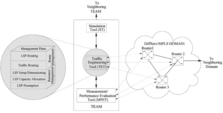
The architecture of the TEAM is shown in Fig. 5. As shown, TEAM has a central server, the traffic engineering tool (TET), which is supported by two tools: simulation tool (ST) and mea-surement/performance evaluation tool (MPET). The TET and the MPET will interact with the routers and switches in the do-main. The MPET will provide a measure of the various param-eters of the network and routers like the available bandwidth, overall delay, jitter, queue lengths, number of packets dropped in the routers, etc. This information will be input to the TET. Based on this measured state of the network, the TET decides the course of action, such as to vary the capacity allocated to a given LSP or to preempt a low priority LSP to accommo-date a new one, or to establish the path for a traffic requiring a specified QoS. The TET also will automatically implement the action, configuring accordingly the routers and switches in the domain. Whenever required, the TET can consolidate the deci-sion using the ST. The ST will simulate a network with the cur-rent state of the managed network and apply the decision of the TET to verify the achieved performance. The TET management tasks include resource management (LSP setup/dimensioning, LSP preemption, LSP capacity allocation) and route manage-ment (LSP routing), as shown in Fig. 5.
VI. PERFORMANCEEVALUATION
In this section, we demonstrate the performance of TEAM and the synergetic interworking of the described techniques and show their operation. The comparison of each TEAM function-ality with current state-of-the-art equivalent techniques has been performed and can be found in our previous work. Since to the
Fig. 5. TEAM framework and functionalities.
Fig. 6. Network topology.
best of our knowledge, there are no other comprehensive net-work managers such as TEAM with such a diverse set of func-tionalities, we compare TEAM to the traditional Internet man-agers.
The following results are obtained by simulating a network consisting of 40 nodes and 64 links, each with capacity of 600 Mb/s, as shown in Fig. 6. This network topology is based on the backbone topology of a well-known Internet Service Provider. The traffic in the network consists of aggregated bandwidth re-quests between node pairs having two possible priorities. The priority level 0 is the lower priority which can be preempted by the higher priority requests of level 1. We model these traffic re-quests with Poisson process arrivals and exponential durations. The set of routing schemes for comparison in SPeCRA includes shortest path, widest shortest path and maximum utility routing. We consider generalized medium traffic load on the network to observe the effects on the network performance and the different actions taken by TEAM in this scenario. We define the
general-ized medium traffic load as traffic matrix with equal values as the elements.
To evaluate the performance of TEAM as the network manager, we consider both the network performance and the complexity associated with TEAM. In particular, for the performance, we consider the rejection of requests, the load distribution, the cost of network measurements, and the cost of providing the service to the requests. The complexity is measured by the number of actions performed by TEAM. We compare these metrics for a network which is managed by TEAM and a network which is managed by a traditional man-ager (TM), like in the current Internet. We assume that in the traditional network management, the MPLS network topology is static and is the same as the physical network. In this case, the shortest path routing algorithm is used for LSP establishment, there is no LSP preemption and there are no online network measurements for adaptive network management.
The simulation was run on a computer with RedHat Linux 7.3, running kernel 2.4.18 on a Pentium III at 800 MHz with 256 MB RAM and 512 MB swap space. The simulation was written in the programming language C. More details about the simulation can be found in [23]. By running the simulations a few times with the generalized medium traffic load, we observed that the LSP setup/capacity allocation (Sections II and III) and LSP routing (Section IV) techniques played a major role. In Fig. 7, we show the rejection ratio for the requests with TEAM and with TM. As we can see, the rejection is 75% lower when TEAM is managing the network. TEAM is able to achieve lower rejection than TM due to the efficient load balancing.
Next, we demonstrate the efficiency of TEAM by comparing the performance with respect to the minimum and average avail-able bandwidths for all the links in the network. In Fig. 8, we plot the minimum available bandwidth. We see that in the absence of TEAM, the network links have lower minimum available band-width as compared to the case when TEAM is active. This is
Fig. 7. Rejection ratio.
Fig. 8. Minimum available bandwidth.
attributed to the fact that the traffic load is evenly distributed in the network using TEAM.
In Fig. 9, we show the average available bandwidth in the network. We see that the values for the case when TEAM is em-ployed are lower than the case when TM is emem-ployed. This gives the false impression that the performance of TEAM in this case is worse than the TM. However, this is not correct and it is still due to the poor load balancing by the traditional network man-ager. In fact, when the load is not well distributed, few links in the network are overloaded and the rejection probability be-comes higher. This observation is corroborated by the high re-jection ratio reported in Fig. 7. Summarizing, the average avail-able bandwidth in the network is lower using TEAM because TEAM is allowing more traffic to be carried.
In Fig. 10, we plot the cost for performing network mea-surements. This cost is assumed to be linearly proportional to the number of available bandwidth measurements in the net-work. From Fig. 10, we see that around 30% of TEAMs ac-tions (like LSP setup, capacity allocation, routing and preemp-tion) required an online measurement. This is compared to the TM where there is no need for network measurement since it is based on SLA contracts and nominal reservations. This mea-surement overhead has been limited to such low values by the
Fig. 9. Average available bandwidth.
Fig. 10. Cost of network measurements.
filtering mechanisms in the individual TEAM techniques and it is offset by the lower rejection of the requests and consequently higher revenue.
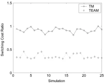
In Fig. 11, we plot the normalized costs of providing ser-vice in the network. It is mainly a representative of the traffic switching cost that can be performed in the MPLS mode or IP mode. As it is well known, it is less expensive to switch traffic in the MPLS mode as compared to the IP mode due to the simpler forwarding mechanism of the MPLS routers. The more the LSPs are created in the network, the lower is the overall switching cost for the traffic. However, the lower switching cost has to be balanced with a high signaling cost attributed to each LSP setup/redimension. Thus, TEAM provides an optimal number of LSPs in the network by balancing the switching and signaling costs. This optimal topology depends on the offered traffic and in this generalized medium traffic scenario, it is not as con-nected as the fully meshed topology. For this optimal topology, the switching cost is approximately 40% of the switching cost with the static network topology. The static topology has the minimum number of LSPs as it corresponds to the physical topology.
Fig. 11. Cost of providing service. TABLE I
TEAM OPERATIONALLOAD
In Table I, we show the TEAM operational load. In other words, the table represents the number of actions performed by TEAM to handle the incoming bandwidth requests. We see that 19% of the requests lead to the activation of the LSP setup/redimensioning procedure whereas only 0.5% of the requests were provisioned after preempting a pre-existing LSP. Most of the LSPs were routed using the shortest path routing algorithm because of the medium traffic load in the network. However, TEAM is able to choose other routing algorithms like widest shortest path and maximum utility to achieve better load balancing in cases when the shortest path route is overloaded.
VII. CONCLUSION
In this paper, we have presented measurement-based tech-niques to adapt the DiffServ/MPLS networks to changing traffic conditions. They include LSP setup, LSP capacity allocation and LSP routing. These techniques are based on well-known adaptive learning theories. In particular, Markov decision processes are the basis of the LSP setup algorithm, Kalman filter theory is used for the LSP capacity allocation and the LSP routing relies on the Stochastic Comparison theory. In addition to these three techniques, we also presented TEAM which is a unified architecture for network management and traffic engi-neering and it is based on the three techniques along with other methods such as LSP preemption. The performance evaluation of TEAM, as compared to traditional network manager, shows that TEAM performs efficient resource and route management in the network by using online measurements of network state and reacting instantly to network changes.
ACKNOWLEDGMENT
The authors would like to thank Dr. Akyildiz for his support and continuous encouragement.
REFERENCES
[1] D. Awduche, A. Chiu, A. Elwalid, I. Widjaja, and X. Xiao, Overview and principles of internet traffic engineering, IETF RFC 3272, May 2002. [2] D. O. Awduche and B. Jabbari, “Internet traffic engineering using
multi-protocol label switching (MPLS),”Comput. Netw., vol. 40, no. 1, pp. 111–129, Sep. 2002.
[3] D. O. Awduche, J. Malcolm, J. Agogbua, M. O’Dell, and J. McManus, Requirements for Traffic Engineering Over MPLS, IETF RFC 2702, Sep. 1999.
[4] F. Le Faucheur and W. Lai, Requirements for Support of Differentiated Services-Aware MPLS Traffic Engineering, IETF RFC 3564, Jul. 2003. [5] F. Le Faucheur, L. Wu, B. Davie, S. Davari, P. Vaananen, R. Krishnan, P. Cheval, and J. Heinanen, Multi-Protocol Label Switching (MPLS) Support of Differentiated Services, IETF RFC 3270, May 2002. [6] G. Armitage,Quality of Service in IP Networks, ser. Technology
Se-ries. New York: MacMillan, 2000.
[7] S. Uhlig and O. Bonaventure, “On the cost of using MPLS for inter-domain traffic,” inProc. QoFIS’00, Berlin, Germany, Sep. 2000, pp. 141–152.
[8] C. Scoglio, T. Anjali, J. C. de Oliveira, I. F. Akyildiz, and G. Uhl, “A new threshold-based policy for label switched path setup in MPLS networks,” inProc. 17th ITC’01, Salvador, Brazil, Sep. 2001, pp. 1–12.
[9] T. Anjali, C. Scoglio, J. C. de Oliveira, I. F. Akyildiz, and G. Uhl, “Op-timal policy for LSP setup in MPLS networks,”Comput. Netw., vol. 39, no. 2, pp. 165–183, Jun. 2002.
[10] A. Terzis, L. Wang, J. Ogawa, and L. Zhang, “A two-tier resource man-agement model for the internet,” inProc. IEEE GLOBECOM’99, Rio de Janeiro, Brazil, Dec. 1999, pp. 1779–1791.
[11] A. Terzis, “A two-tier resource allocation framework for the internet,” Ph.D. dissertation, Univ. California, Los Angeles, CA, 2000. [12] C. N. Chuah, L. Subramanian, R. H. Katz, and A. D. Joseph, “QoS
provi-sioning using a clearing house architecture,” inProc. 8th Int. Workshop on Quality of Service, Pittsburgh, PA, Jun. 2000, pp. 115–124. [13] N. G. Duffield, P. Goyal, A. Greenberg, P. Mishra, K. K. Ramakrishnan,
and J. E. van der Merwe, “A flexible model for resource management in virtual private networks,” inProc. ACM SIGCOMM’99, Cambridge, MA, Sep. 1999, pp. 95–108.
[14] “White Paper: Cisco MPLS AutoBandwidth Allocator for MPLS Traffic Engineering,”, http://www.cisco.com/warp/public/cc/pd/iosw/ prodlit/mpatb_wp.pdf, Jun. 2001.
[15] T. Anjali, C. Scoglio, and G. Uhl, “A new scheme for traffic estimation and resource allocation for bandwidth brokers,”Comput. Netw., vol. 41, no. 6, pp. 761–777, Apr. 2003.
[16] P. S. Maybeck, Stochastic Models, Estimation, and Control. New York: Academic, 1979.
[17] R. Guerin, A. Orda, and D. Williams, “QoS routing mechanisms and OSPF extensions,” inProc. IEEE GLOBECOM’97, Phoenix, AZ, Nov. 1997, pp. 1903–1908.
[18] Z. Wang and J. Crowcroft, “Quality-of-service routing for supporting multimedia applications,”IEEE J. Sel. Areas Commun., vol. 14, no. 7, pp. 1288–1234, Sep. 1996.
[19] D. Eppstein, “Finding thekshortest paths,”SIAM J. Comput., vol. 28, no. 2, pp. 652–673, 1998.
[20] G. Apostolopoulos, R. Guerin, S. Kamat, and S. K. Tripathi, “Quality of service based routing: A performance perspective,” inProc. ACM SIG-COMM’98, Vancouver, BC, Canada, Sep. 1998, pp. 17–28.
[21] K. Kar, M. Kodialam, and T. V. Lakshman, “Minimum interference routing of bandwidth guaranteed tunnels with MPLS traffic engi-neering application,”IEEE J. Sel. Areas Commun., vol. 18, no. 12, pp. 2566–2579, Dec. 2000.
[22] J. C. de Oliveira, F. Martinelli, and C. Scoglio, “SPeCRA: A stochastic performance comparison routing algorithm for LSP setup in MPLS net-works,” inProc. IEEE GLOBECOM’02, Taipei, Taiwan, Nov. 2002, pp. 2190–2194.
[23] C. Scoglio, T. Anjali, J. C. de Oliveira, I. F. Akyildiz, and G. Uhl, “TEAM: A traffic engineering automated manager for diffserv-based MPLS networks,”IEEE Commun. Mag., vol. 42, no. 10, pp. 134–145, Oct. 2004.
[24] M. L. Puterman,Markov Decision Processes: Discrete Stochastic Dy-namic Programming. New York: Wiley, 1994.
[25] V. Jacobson, Pathchar, 1997.
[26] M. Jain and C. Dovrolis, “End-to-end available bandwidth: Measure-ment methodology, dynamics, and relation with TCP throughput,” in
Proc. ACM SIGCOMM’02, Pittsburgh, PA, Aug. 2002, pp. 295–308. [27] , “Pathload: A measurement tool for end-to-end available
[28] [Online]. Available: http://people.ee.ethz.ch/oetiker/webtools/mrtg/ [29] T. Bonald, S. Oueslati-Boulahia, and J. Roberts, “IP-traffic and QoS
con-trol: Toward a flow-aware architecture,” inProc. 18th World Telecommu-nication Congr., Paris, France, 2002.
[30] J. W. Roberts, “Traffic theory and the internet,”IEEE Commun. Mag., vol. 39, no. 1, pp. 94–99, Jan. 2001.
[31] L. Kleinrock,Queueing Systems. New York: Wiley, 1975.
[32] L. Dai and C. H. Chen, “Rates convergence of ordinal comparison for dependent discrete event dynamic systems,”J. Optim. Theory Applicat., vol. 94, no. 1, pp. 29–54, Jul. 1997.
Tricha Anjalireceived the (Integrated) M.Tech. de-gree in electrical engineering from the Indian Insti-tute of Technology, Bombay, in 1998 and the Ph.D. degree from the Georgia Institute of Technology, At-lanta, in 2004.
She is currently an Assistant Professor in the Electrical and Computer Engineering Department, Illinois Institute of Tecnology, Chicago. Her research interests include design and management of MPLS and optical networks.
Caterina Scoglioreceived the Dr. Ing. degree in elec-tronics engineering and the postgraduate degree in mathematical theory and methods for system anal-ysis and control from the University of Rome “La Sapienza,” Italy, in 1987 and 1988, respectively.
From 1987 to 2000, she was a Research Scientist with Fondazione Ugo Bordoni, Rome. From 2000 to 2005, she was a Research Engineer with the Broad-band and Wireless Networking Laboratory, Georgia Institute of Technology, Atlanta. Currently, she is an Associate Professor in the Electrical and Computer Engineering Department, Kansas State University, Manhattan. Her research in-terests include optimal design and management of multiservice networks.
Jaudelice Cavalcante de Oliveira(M’98) received the B.S.E.E. degree from Universidade Federal do Ceara (UFC), Ceara, Brazil, in 1995, the M.S.E.E. degree from Universidade Estadual de Campinas (UNICAMP), Sao Paulo, Brazil, in 1998, and the Ph.D. degree in electrical and computer engineering from the Georgia Institute of Technology, Atlanta, in 2003.
In 2003, she joined the Department of Electrical and Computer Engineering, Drexel University, Philadelphia, where she is currently an Assistant Professor. Her research interests include the development of new protocols and policies to support fine grained quality of service provisioning in the future Internet, traffic engineering techniques, and the design of solutions for efficient routing in ad hoc and sensor networks.