Endogenous structural change and climate targets.

Full text

(1)1. Endogenous Structural Change and Climate Targets Modeling experiments with Imaclim-R*. Renaud Crassous, Jean-Charles Hourcade, Olivier Sassi **. This paper envisages endogenous technical change as resulting from the interplay between the economic growth engine, consumption, technology and localization patterns. We perform numerical simulations with the recursive dynamic general equilibrium model IMACLIM-R to study how modeling induced technical change affects costs of CO2 stabilization. IMACLIM-R incorporates innovative specifications about final consumption of transportation and energy to represent critical stylized facts such as rebound effects and demand induction by infrastructures and equipments. Doing so brings to light how induced technical change may not only lower stabilization costs thanks to pure technological progress, but also triggers induction of final demand effects critical to both the level of the carbon tax and the costs of policy given a specific stabilization target. Finally, we study the sensitivity of total stabilization costs to various parameters including both technical assumptions as accelerated turnover of equipments and non-energy choices as alternative infrastructure policies.. *. The authors are indebted to Jonathan Khoeler, Misato Sato and Michael Grubb for their helpful collaboration on this paper. The development of the IMACLIM-R model results from a collective effort at CIRED to develop a recursive version of the IMACLIM-S model (Ghersi et al., 2003). It benefited from the sound contribution of Philippe Ambrosi, Vincent Gitz and Meriem Hamdi-Cherief. ** CIRED - Centre International de Recherche sur l’Environnement et le Développement 45 bis avenue de la Belle Gabrielle 94736 Nogent sur Marne Cedex contact : crassous@centre-cired.fr.

(2) 2. 1. Introduction. This paper revisits the comparison between autonomous (ATC) and endogenous (ETC) models of technical change from a specific premise: in a model where policy signals induce the rate of technical change (through both learning by doing and investments in R&D) the behavior of households’ consumption must necessarily be taken into account. This premise is one made in the context of a wider discussion on how to endogenize structural changes in economic growth models. The notion that the rate and direction of technical progress (in terms of aggregate factor intensity) depend not only on the efficiency of physical capital but also on the structure of final households’ demand has been put forward by Solow (1990). Economic history has also demonstrated the importance of the interplay between these two parameters (Wright, 1990). In this paper, parameters such as product differentiation (Barro and Sala-i-Martin, 1998) in non energy related goods and services are not endogenized, and we assume static private and public preferences for enduse services. But we try and contribute to the discussion of endogenous structural changes by explicitly addressing the interplays between the endogenous growth engine, decarbonization policies and the transportation dynamics as a critical component of final demand. More specifically, we attempt to capture the rebound effects on gasoline demand triggered by efficiency gains of vehicles as well as the mobility needs induced by infrastructure choices for given consumer preferences. In this way, we attempt to extend the concept of ETC to the interplays between innovation, infrastructure and energy consumption (Hourcade, 1993). To disentangle the many facets of ETC vs. ATC debate, we conduct numerical experiments assuming: i) the absence of carbon free gasoline as a backstop by the end of the century; ii) no “negative costs potentials” and no carbon sequestration; iii) a linear carbon tax profile (hence sub-optimal in all simulations) and iv) no possibility of early retirement of capital stocks. The results from such exercise magnifies effects of the key factors at play (at the expense of high GDP losses for meeting tight GHG concentration targets as 450 ppm in some policy scenarios)1, with the advantage of delivering some novel insights on the policy variables capable of minimizing costs of such ambitious targets. This papers is structured as follows. Section two describes the rationale of the IMACLIM-R framework and how it describes induced technical change mechanisms (ITC). Section three presents the baseline scenario. In section four, we explain why assuming that the same overall potentials of technical change may or may not be policy-induced leads to very different costs assessments of stabilization scenarios. We pay particular focus on the demand induction in transportation as well as on the crowding-out effect of investments. Sensitivity tests are performed in the fifth section to enlight the underlying mechanisms. The sixth section provides additional insights into the control of mobility.. 1. Note, however, that some of the assumptions retained for these simulations are far from being implausible. For example, the assumption of cheap carbon-free gasoline by the middle of the 21st century would dampen effects of some of the mechanims at play, which may in turn have a critical role in the absence of this optimistic assumption..

(3) 3. 2 2.1. The IMACLIM-R modeling framework Structure of the model. IMACLIM-R is a multi-sector multi-region recursive growth model projecting, on a yearly basis, the world economy up to 2100. It is run for five regions (the four SRES regions – OECD90, REF, ASIA, ALM 2 – from which we set apart the OPEC region), 10 economic sectors (coal, crude oil, natural gas, oil products, electricity, construction, composite good, air transport, sea transport, terrestrial transport) and two transport modes auto-produced by households (personal vehicles and non-motorized transportation). The model uses a recursive dynamic framework3 where economic pathways are represented through a sequence of static general equilibria, linked by dynamic equations (Figure 1). These successive equilibria are computed under the constraints imposed by the availability of production factors and inter-sectoral technical relations at each point in time. The outcome is a set of values (output levels, price structure, investment) sent to dynamic equations which represent population dynamics, fossil fuel resources depletion and technical change. Technical change encompasses overall labor productivity and technical coefficients and results in a new production frontier used to compute the subsequent equilibrium. In an ATC framework, the new parameters of this new production frontier come from exogenous trends whereas under ETC assumptions, they come systematically from endogenous relations between cumulated investments and technical progress. This approach was developed in an effort to address four interrelated challenges: i) to incorporate some of factors that drive economic growth, rather than defining growth rates through entirely exogenous assumptions; ii) to utilise in a consistent manner bottom-up expertise about technical change; iii) to allow for the description of imperfect foresight (about future relative prices, final demand and profitability) and of possible decision routines4 in infrastructure sectors; iv) to capture possible transition costs towards long run equilibria, transition costs that may result from the interplay between non perfect foresight and the inertia of technical systems. The framework also allows us to a) represent baseline scenarios which can have a non-optimal use of production factors (structural unemployment, excess capacity or capacity shortages5) and b) to account for the fact that economies adapt to climate targets within the constraints imposed by past decisions, including transaction costs of changing domestic social contracts. The model incorporates mechanisms driving the economy back to stabilized trajectories which are reached if steady long term signals are given to the agents (carbon and oil prices) and when the influence of inertia progressively recedes. 2. See (IPCC, SRES, 2000) or http://www.grida.no/climate/ipcc/emission/149.htm for a full description of these regions. Similar to the option followed by EPPA (Paltsev et al., 2005 for the last version) or SGM (Edmonds et al., 1993) for instance. 4 The notion of decision routines encompasses here seemingly non optimal choices due to the influence of institutional contexts and/or the incorporation of non economic objectives (equity, security) in public decisions. 5 Picturing non-optimal baselines and policies is important in the context of developing countries since underdevelopment is the product of institutional and market failures (for that reason current work at CIRED aims to include public indebtedness in long-term simulations). It is also important for developed countries; for example the 4% GDP loss predicted in some studies as a cost of Kyoto target for the US relied specifically on the assumption of non-optimal responses (IPCC, TAR, WGIII). 3.

(4) 4. Time path. Static equilibrium t+1. Static Equilibrium t. Updated parameters (tech. coef., stocks, etc.). Bottom-up sub-models Capital and technology dynamics Demography. Price-signals, Investments Physical flows. Figure 1 : the recursive dynamic framework of IMACLIM-R. In this modeling system, all flows are tracked at each point in time, by a double accounting in both money metric values and in physical quantities, the two being linked by relative prices6. This hybrid accounting is used to by-pass difficulties linked to the representation of capital in usual production functions: at a given point, the model accounts for the available physical capacities of production and describes the financial flows serving to replace and expand them (see 2.2. herebelow). It is worth noting that, in addition to facilitating the tracking of the sources of GHG emissions and of the dipping into fossil fuel resources, this methodology facilitates a transparent incorporation through physical technical coefficients of bottom-up information regarding (i) the technical saturations of efficiency gains in energy and transportation equipments at a given time horizon and (ii) how the technical characteristics of energy (and transportation) systems react to relative price variations.. 2.2. Static equilibrium under a given production frontier. Each static equilibrium is Walrasian in nature: it is characterized by annual flows of goods and money and a set of relative prices as they results from supply and demand behaviors, investment decisions, private and public income budget constraints and clearance conditions for international and national markets. The calibration of the static equilibrium at the benchmark year (2000) is based on data from the following sources: social accounting matrices form the GTAP Database Version 5; IEA/OECD physical database for energy, and. 6 The flows of the five energy goods are expressed in Mtep; final consumption of transportation is indexed in terms of passenger-kilometers; housing area is tracked in terms of square-meters built..

(5) 5 data from Schäfer and Victor (2000) and the World Road Statistics database for transportation. The following is assumed for the current period, in order to solve for subsequent periods: (i) Producers are constrained by fixed capacities (the depreciated sum of previous vintages) and the technical characteristics of the equipment stock that result from past decisions. This comes to a putty-clay assumption. Hence, the variables of the model are prices p, wages w and utilization rate linked to the level of output (UR). Average production costs thus derive from fixed input-output coefficients ICj, a fixed labor intensity l, and a static diminishing return factor ΩUR which is function of a flexible capacity utilization rate. A constant mark-up π is added to the mean cost7. For primary energy sectors, the mark-up increases in function of cumulated production, as to capture the scarcity rent on the longrun.. (. ). UR p = ∑ p IC ⋅ w ⋅l +π ⋅ p j ⋅ IC j + Ω. (1). j. with. UR =. Q Cap. (2). Equation (1) in fact represents the inverse supply curve of each sector, since it shows how the representative producer decides its level of ouput Q (Q<Cap) in function of all prices and wages. The desired level of ouput in each sector implies a labor demand l·Q. The difference between total labor demand across all sectors and the current labor force8 is unemployment. The level of unemployement has an impact on real wages through regional wage curves: wages tend to infinity as unemployment disappears and they tend to zero as unemployment rate tends to one. The calibration of these wage curves rests on Blanchflower and Oswald (1995). (ii) Consumers’ final demand is derived by solving the utility maximization problem for a representative consumer :. MaxU =. ξ ∏(C -bn ) ⋅ (S i. i. − bnhousing) housing ⋅ (Smobility − bnmobility) mobility ξ. housing. ξ. (3). goods i (composite, construction). (. with S mobility = CES pkmair , pkmpublic , pkmcars , pkmnon motorized. ). (4). In equation (3), C holds for consumed quantities of composite and construction, S holds for services provided by energy and mobility, bn corresponds to the basic needs of final consumers for final goods and services and pkm represents the physical consumption of each mode of transportation accounted in terms of passenger-kilometers. Note first that energy does not directly enter the utility function; it contributes to welfare through the services it fuels. The demand for these services is driven by private housing and transportation equipments. Energy consumption is then dependent upon the 7. Such a constant markup corresponds to a profit-maximizing decision of producers when the diminsihing return factor follows an exponential function of utilization rate. 8 Active population follows exogenous trends for each region and incorporate fixed migration flows. These parameters are kept constant between the baseline and policy secenarios...

(6) 6 efficiency coefficients characterizing the existing stock of end-use equipments. Second, transportation modes are nested in a single index of mobility defined by equation (4). To account for preferences and spatial heterogeneity of their availability, the different modes of transport are assumed to be imperfect substitutes. Equation (3) is maximized subject to income and time constraints. Income, defined by equation (5) equates the sum of savings, the energy bill (induced by residential needs and private transportation) and expenditure on other goods and services (including public transportation). Savings follow an exogenous saving rate. The time constraint (6) is derived from empirical findings (Zahavi and Talvitie, 1980). and represent average daily travel time of a household. For a given travel mode, the marginal consumption of time per kilometer τ is an invert correlated to the congestion which, for a given mobility demand, depends on the availability and efficiency of infrastructures and equipments.. Income = S +. ⎛ ⎞ pi ⋅ Ci + ⎜ ∑ pEi ⋅ α Eihousing ⋅ stock m ² ⎟ non − energy ⎝ energies Ei ⎠ non − transport. ∑. (5). goods i. ⎛ ⎞ + ⎜ p public ⋅ pkm public + pair ⋅ pkmair + ∑ ( pkmcars ⋅ α Ficars ) ⎟ Fuels Fi ⎝ ⎠. Tdisp =. ∑ ∫. Modes Ti. pkm Tj. 0. τ j (u )du. (6). Ultimately modal shares and mobility demand that result from utility maximization depend on both travel costs and travel time productivity of the various modes (average km traveled per unit of time). Through this channel, the quantity and cost efficiency of infrastructure stocks and the energy efficiency of vehicles have an impact on mobility demand, as well as the trade-off between mobility and other goods and services. (iii) Investment allocation across regions and sectors is governed by the expectations of future profits. Part of the regional savings are reinvested domestically, the rest being redirected to an international capital pool, which in turn re-allocates them to regions according to the sectors’ profitability. Allocation of investments does not, however, equalize the marginal productivity of new investments because investors account for idiosyncratic country-risk9. Future profits are imperfectly foreseen, as decision-makers interpret the current economic signals as the best available information about present and future economic conditions. Sub-sector allocation of investments across technologies are treated in the dynamic equations. (iv) The equilibrium clears international markets for goods and capital. A conventional ‘Armington’ specification (Armington, 1969) is adopted for non energy goods though energy goods are considered to be homogenous commodities. Their trade rests on specific market shares and real physical account of quantities10. Capital and trade balances compensate each other, through variations of all regional prices11.. 9. ‘Country risks’ represents the aggregate relative economic attractiveness of regions. Armington specifications do not allow to sum physical quantities that are imported and produced domestically, since they are supposed to be different kind of goods. 11 The variation of regional price index can be interpreted as implicit flexible exchange rates. 10.

(7) 7 The existence of short term constraints on the physical capital and technical coefficients implies that market clearing is made through modifications to relative prices and sectoral level of output. The equilibrium is thus second best and allows for capacity shortages, overcapacity and unemployment. The new relative prices impact on profitability rates and investment allocation. Inside each region, investments are converted into new productive capacities through a regional β-matrix12, which allows for calculating the price of a new unit of production capacity for each sector. The over or under-employment of factors of production can thus be released across time thanks to these investments and related incorporated technical change.. 2.3. From static equilibria to growth dynamics:. As pictured in Figure 1, dynamic equations encompass both the evolution of the production frontier and movement along this frontier (input-output coefficients, sectorspecific installed capital, public infrastructures, labor force) and of the constraints impinging upon the consumers program (income, end-use equipments). They capture the joint effect of the macroeconomic growth engine and technical changes on the supply and demand-side. The growth engine is composed of (i) exogenous demographic trends (UN estimations corrected by migration flows so that populations of low fertility regions are stabilized) (ii) labor productivity changes (the labor intensity l in equation (1) and fueled by (i) regional saving rates (ii) investments allocation across sectors. Even though they do not affect longrun growth rates, such as in the Solowian models, short term adjustments condition output growth on the short and medium term. Productivity can be assumed either to follow an exogenous trend (w/o ITC) or to be driven by cumulated investment in the composite good sector (with ITC), accounting for an investment externality on all other sectors. In both cases the parameters are calibrated on historic trajectories (Maddison, 1995) and ‘best guess’ of long-term trends (Oliveira-Martins et al., 2005). In addition, the β-matrix values are increased to account for the part of productivity gains that comes from capital deepening13. Technical change at a sector level (intermediate or end-use efficiency gains, costs of new technologies and substitutions between energy sources) are driven by the interplay between changes in relative prices and cumulated investments. Relative prices operate in the same way in both versions of the model by affecting choices of both firms and consumers in purchasing new equipments (the resulting new values of their energy and mobility demand being captured in the following static equilibrium). The calculation of the production frontier is based on a putty-clay assumption which implies that technologies are embodied in the equipment stocks resulting from the cumulated investment vintages. In the ‘w/o ITC’ version, the diffusion of autonomous technical change is thus constrained by the pace of replacement of capital. This creates short run inertia, which is considered realistic for energy, transportation and heavy industry sectors. With ITC, this pace is also binding with the difference that ‘learning-by-doing’ and R&D mechanisms are also positively correlated to cumulated investments. It is thus possible to accelerate the efficiency gains in energy and composite sectors (7) and the decrease of investments costs of carbon-free techniques (8). In. 12. With βi,j the physical amount of good i that is necessary to build in sector j the capacity to produce one physical unit of good j. 13 The link beween labor productivity gains and capital deepening is calibrated on historical data gathered by (Maddison, 1995)..

(8) 8 addition, changes in relative prices of energy induce efficiency improvements in private cars, end-use equipments and in the composite sector. IMACLIM-R, in some sense, describes such mechanisms through ‘reaction functions’, for example, through reduced forms of bottom-up information. It computes the evolution of coefficients of the technical input-output matrix, end-use efficiencies (7) and β-matrixes coefficients (8) in function of historical investments, as well as variations of relative prices: - endogenous variations of energy efficiency of production capacities and equipments: ⎛ t ⎞ (t ) ⎟ Energy Efficiency(t) = f ⎜⎜ ∑ Investments, ∆penergy ⎟ ⎝ τ =t0 ⎠. f Σ′I > 0, f ∆′p > 0 (7). - endogenous variations of investments costs for carbon saving equipments (learning by doing and R&D):. ⎛. ⎞. t. β i(,tj+,1k) = g ⎜⎜ ∑ Investments k(τ, )j ⎟⎟ τ =t ⎝. 0. ⎠. g Σ′ I < 0. (8). for any low carbon energy j in country k and any investment good i Such functions are calibrated on (i) explicit views of technical potentials in the form of asymptotes on energy efficiencies and on the shares of given energy carriers in end-use demand and energy supply, and (ii) on results from bottom-up models. They incorporate technical asymptotes translating expert judgments about the ultimate potentials of each technical bundle. In the base case experiment of this exercise we used the following estimates14: in the electric sector, the technical asymptotes for energy efficiency are set at 0.5 for coal-based technologies, 0.6 for oil and gas technologies (these figures do not reflect the potential efficiency gains from cogeneration ); the carbon content of energy mix is likely to fall to zero. With ITC, the rate of decrease of the price of non-carbon energies doubles when investment in those technologies is multiplied by four with respect to the reference case. In the composite sector, the rate of global energy efficiency improvement doubles if the energy prices increases by 60%, and the energy mix can be decarbonized up to 100% by 2100. For the residential consumption of energy, maximum efficiency gains are -2% per year. For transportation, the maximum average efficiency of cars and trucks in 2100 is set at 25% of today’s best available techniques.. 2.4. Stabilization of CO2 concentrations. To date IMACLIM-R does not include a climate model, then we use total carbon budget over the century as a proxy for the stabilization level15. We have checked ex post that the emissions trajectories we derived from these carbon budget are consistent with expected stabilization, using the carbon cycle and climate module developed at CIRED (Ambrosi et al., 2003).. 14. The estimates we used reproduce orders of magnitude from experts judgments (IEA Investment Oultook, 2004) and from output of the POLES energy model. 15 Since in the 550 ppm scenarios stabilization would occur after 2100, the budget over the 21st century is only a necessary condition for stabilization..

(9) 9 3. The reference scenario: slow catching-up, carbon intensive development patterns. IMACLIM-R is not designed to follow an ex-ante scenario, but rather to produce its own reference scenario from a set of upstream assumptions regarding labor productivity growth, demography or international trade. To try and calibrate it on the CPI baseline would require a cumbersome process of selecting one ad hoc set of parameters. On the charts in appendix A, the dotted lines give the trends of the potential growth of each region (sum of input assumptions of productivity and population growth) and the black line gives the real GDP growth. These curves follow rather similar trends, their differences being due to the functioning of the world markets (goods, energy, capital). ASIA and REF, after an acceleration of their economic growth in the first part of the century, converge to growth rates on the same order of magnitude as OECD, whereas the economic growth rate re-accelerates in ALM after 2070 because the catching up of most African countries is delayed by comparison with ASIA. At the end of the century the trend towards some form of steady growth is interrupted due to the sharp increase of oil prices: the transition costs to this new setting explain why the real GDP growth of all regions, OPEC excepted, become lower than the sum of input assumptions regarding productivity and population. This reference case generates 25 GtC of emissions in 2100 and a cumulated 1677 GtC carbon release over the century. This results from three main components to be borne in mind when analyzing the cost of stabilization scenarios. a) the increase of households final consumption shows a significant but modest and regionally very heterogeneous catching up between 2000 and 2100 (see table in appendix B) : (i) the mean annual growth rate of per capita consumption of composite goods is 1.37% in OECD, 1.87 % in ASIA, 2.67 % for REF, 1.25 % for ALM and 1.63 % for OPEC16; (ii) per capita housing space is multiplied by 2.5 in OECD, 4 in ASIA, 6 in REF; (iii) per capita total mobility doubles in OECD, triples in ASIA and quadruples in REF. The growth of the traffic volume rests on different modal breakdowns across regions: in non-OECD countries mobility growth is mainly due to an increasing access to motorized mobility (public modes initially, followed by private cars when welfare increases), while OECD experiences a shift to air transport. b) the decoupling between economic growth and energy demand ranges between 0.66% to 0.98% per year depending upon regions. Chart in appendix C displays information about the relative role of structural change and energy efficiency gains in this decoupling. For OECD, the decoupling comes mostly from the increasing proportion of services in the composite good (-0.76% per year against -0.12% for energy efficiency after 2050) while for ASIA, ALM and OPEC it comes primarily from energy efficiency gains (-0.5% over the century). This translates the fact that, in these regions the ‘dematerialization’ of the economy takes place only in the second part of the century. c) the aggregate carbon content of the energy supply increases slightly in the first half of the century since the electricity supply rests mostly on coal and gas, fuel for transportation is still dominantly produced from conventional and non conventional oil. In the second half of the 16. Growth rates of developing countries may appear low compared to current trends. In fact this is a mean growth rate over the century, that masks high growth rates during the first half of the century and a generalized slowdown of growth due to the combination of a downward convergence of labor productivity growth to a 2% annual rate and of the ageing of population, especially in Asia..

(10) 10 century fossil fuel prices start rising more significantly, with a “peak oil’ between 2080 and 2090 17. This triggers more significant penetration of non-fossil energy at the end of the century. Thus part of the potential of decarbonization is already included in the baseline, but this a minor part. 4. Policy scenarios: why does ITC make a difference ?. Running IMACLIM-R with or without ITC obviously makes a difference for the dynamic component of the model. One precondition for comparing the two treatments of technical change is to guarantee that they describe identical no-policy baselines and the same degree of pessimism or optimism regarding technical change potentials. For the ‘w/o ITC’ simulations we switched off all the ‘ITC’ components and we calibrated exogenous technical change coefficients to reproduce the same trends of technical change as in the ‘with ITC’ baseline. This treatment encompasses all kinds of technical change: general trend of labor productivity, energy mix, energy efficiency on supply and demand sides, and costs of equipments for non-fossil sources of electricity. Table 1 summarizes the costs assessment of meeting various CO2 concentration targets for OECD and non-OECD regions with a policy based on a carbon tax which increases linearly from 2005 to 210018, and the product of which is recycled first by lowering preexisting taxes on labor and second with lump-sum transfers to households. In our central case, meeting a 550 ppm target requires a 115 $/tC and 384 $/tC carbon tax in 2100 with ITC and without ITC respectively. The 450 ppm target requires 365 $/tC and 1166 $/tC carbon prices with ITC and without ITC respectively. with ITC. Tax profile Carbon price in 2100 OECD losses in Composite consumption Non-OECD losses in composite consumption 19. without ITC. 550 ppm. 450 ppm. 550 ppm. 450 ppm. + 1.5$/ton of C/year. + 3.8 $/ton of C/year. + 4 $/ton of C/year. +12.15$/ton of C/year. 115 $ per ton 365 $ per ton 384 $ per ton of C of C of C. 1166 $ per ton of C. -0.9 %. -3.7 %. -4.6 %. -10.1 %. -2.0 %. -5.6 %. -5.6 %. -13.2 %. Table 1: Costs of CO2 stabilization targets under various technical change assumptions (5% discount rate).. 17. This derives from the cost assessment of conventional and non conventional oil resources provided by the Institut Français du Pétrole. It does not mean that there will be no upward pressure on oil prices up to 2080, due to the geopolitical tensions triggered by geographical polarization of oil resources, but the shocks cause by these tensions have not been incorporated in the baseline utilized in this paper. 18 A ‘benevolent planner’ should impose a 100-years tax profile very different under with or w/o ITC specifications. We did not address this discussion in this paper and used a linear profile in both cases kind in order to concentrate on the differences in the economic mechanisms at work with and w/o ITC. 19 These large losses also encompass larger losses due to lower exports of oil and gas by OPEC and REF regions, which deteriorates commercial balance for those regions..

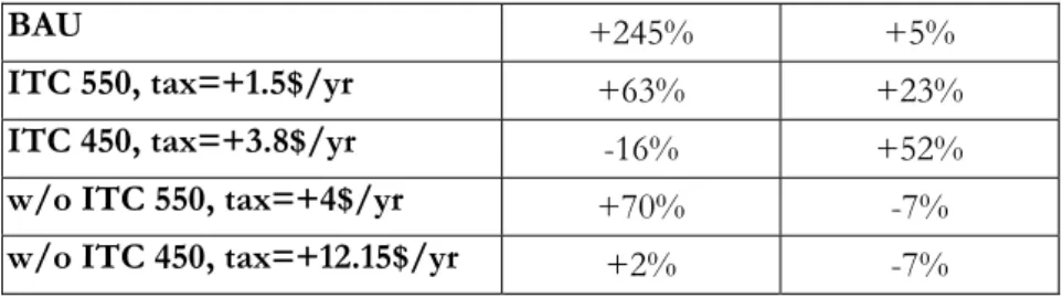
(11) 11 The tax levels mentioned above cause significant consumption losses, far higher without ITC, than those published in the post-SRES IPCC scenarios (IPCC,2001). This is due to conservative assumptions behind our central case; these assumptions are supported by the consideration of limits to large scale deployment of renewable energies (bio-fuels), concerns about nuclear energy, and the inhibition of investments by uncertainty about the ultimate performance of alternative technological routes. The sensitivity analysis conducted in Section 5 discusses these assumptions and considers also assumptions that yield lower costs. First however, we concentrate on the mechanisms governing the differences in the cost assessments delivered with or w/o ITC.. 4.1. Lower carbon prices with ITC despite demand induction. In all simulations, the carbon tax triggers a move towards low carbon intensive production and consumption through energy switching to cleaner fuels and improved energy efficiency. The tax levels required for a given target are determined by the substitution possibilities on both the demand and supply sides at each point in time over the course of a century. The difference in results with and w/o ITC lies in the dynamics of these substitution possibilities. Without ITC, substitution possibilities are moved forward by the autonomous progress coefficients of carbon saving techniques and by the turnover of capital equipment which limits the pace of penetration of these techniques. The tighter the targets, the higher the required carbon price, in order to foster larger substitutions. This hampers sectors’ profitability, lowers economic growth, and triggers a vicious circle; reducing the replacement rate of equipment in turn slows down the penetration of lower costs carbon saving techniques. With ITC, this mechanism is in part offset: the higher the taxes, the quicker the decrease of costs of carbon saving techniques and the higher the pace of their incorporation in the equipment stock. Moreover, ITC incoporates an additional degree of freedom since any increase in energy costs induces some energy efficiency improvements for the entire stock of equipment in the composite sectors. In the long term, for a given level of carbon tax, the difference in carbon intensity between capital stocks with and w/o ITC is substantial. However, behind this quantitatively dominant mechanism, more complex dynamics are at play in the transportation sector. Table 3 displays results which come as expected for the first half of the century: the increase of emissions from transportation is limited to 63% with ITC instead of 70% without ITC in a 550 ppm scenario, even for a 2.5 times lower carbon tax with ITC. This results from accelerated induced efficiency gains in vehicles. Yet these gains are in part offset by a countertendency which is fully revealed after 2050. The availability of more efficient transport infrastructures, including roads and the lower user cost of private vehicles, induces a higher mobility demand. This modifies the transportation breakdown. In the OECD the induced energy efficiency gains partially offset the burden of the tax and households reallocate part of their budget to air travel. In non-OECD regions, these gains mainly facilitate the access to motorized mobility. After 2050, energy efficiency of vehicles reaches an asymptote and the countertendency prevails: in both the 450 and 550 ppm scenarios with ITC, demand for gazoline still increases while it decreases in scenarios without ITC. Change in CO2 Emissions 2000-2050. 2050-2100.

(12) 12 BAU. +245%. +5%. ITC 550, tax=+1.5$/yr. +63%. +23%. ITC 450, tax=+3.8$/yr. -16%. +52%. w/o ITC 550, tax=+4$/yr. +70%. -7%. w/o ITC 450, tax=+12.15$/yr. +2%. -7%. Table 2: Variations of carbon emissions from transportation sector. Note: Under ‘BAU’, emissions from transport by 2100 almost return to 2050 levels, due to the depletion of oil resources and a sharp increase of fuel prices during this period. Thus, to the final consumers that face relative cost of higher mobility (a rebound effect), price signals are weakened by price-induced efficiency gains in ‘with ITC’ scenarios. Morover, since mobility demand causes important infrastructure investments characterized by a high inertia, this may create the risks of ‘lock-in’ to carbon-intensive transportation systems, putting an increased burden on other sectors (Lecocq et al., 1998). This raises the issue of policy instrument choice on shapping transportation dynamics. We come back to this issue in the fifth section.. 4.2. From carbon taxes to variations of economic growth. Aggregate costs of stabilization targets with or without ITC differ in a way which is globally consistent with the carbon prices profiles of each scenario: 1.1 % decrease of the discounted sum of households’ consumptions of composite goods (a proxy for welfare losses) with ITC against 4.8 % without ITC for a 550 ppm target. However a deeper scrutiny reveals that the relation between the tax level and the consumption losses are far from being linear and homogeneous. First, in both scenarios, losses are higher in non-OECD countries (2.0% and 5.6% against 0.9% and 4.6%) despite a consistent carbon tax in both regions. Secondly, for a carbon tax 2.66 times lower with ITC than without ITC, consumption losses are divided by 5.1 in OECD countries, and by 2.8 in developing countries. The quantitative relation between a given level of carbon tax and consumption losses results from the interplay between two main channels. First, at any static equilibrium, the carbon tax lowers the purchasing power of households and causes a decrease of the demand for composite goods. As shown in Table 3, the impact of a given tax level is lower with ITC than without ITC because ITC triggers higher energy efficiency gains in end-use equipments (residential and vehicles) and a lower carbon content of energy production20. Scenarios BAU ITC Tax=2,5 / 550ppm ITC Tax=3.8 / 450 ppm w/o ITC Tax=4 / 550 ppm w/o ITC Tax=12.15 / 450ppm. 2050 +0% +10% +17% +169% +465%. 2100 +0% -15% +11% +135% +529%. Table 3: variation of energy costs borne by OECD households w.r.t. the reference case. 20. Energy prices are also lower with ITC because of lower demand due to additional energy efficiency gains..

(13) 13 Note: In policy scenarios the rise of oil prices due to resources scarcity is postponed compared with the baseline. This counterbalances the impact of the carbon tax on households energy bill, and even leads to a net gain in 2100 for a 550 ppm target with ITC. The same observations hold for variations of the share of energy costs in total composite production costs (Table 4). The second channel is the impact of carbon saving investments on the overall technical change. Without ITC, lowering investments in the composite goods has the simple effect of slowing down the pace of turnover of equipments and the extension of production capacities. With ITC on the other hand, the overall productivity is also affected, leaving the door open to the crowding out effect observed in theoretical models (Smulders, 2003). Scenarios BAU ITC Tax=2,5 / 550ppm ITC Tax=3.8 / 450 ppm w/o ITC Tax=4 / 550 ppm w/o ITC Tax=12.15 / 450ppm. 2050 +0% +63% +115% +186% +397%. 2100 +0% +0% +1% +91% +126%. Table 4: variation of the share of energy in total production costs of composite goods (w.r.t. the reference case). The magnitude of the slowdown of labor productivity is very low in 550 ppm scenarios: from 1.197 to 1.194 % per year for OECD and from 1.92 to 1.90 % per year for non-OECD countries. Annual labor productivity growth falls more significantly to 1.16% per year and 1.86% per year respectively, but this slowdown is still only responsible for a very minor part of total consumption losses (0.3% and 0.6% respectively). This suggests that the impact of the crowding-out of investments on growth is far less important than the constraints on households budget and sectors’ profitability. 5. Is technological optimism enough to lower costs?. In the simulations above the costs of reaching a stabilization target are contingent upon the transitional tensions in energy markets provoked by the carbon tax, affecting final consumption, sector profitability and overall labor productivity. Coming back to the question that motivates this paper, it now matters to check to what extent such tensions are sensitive only to changes in the available set of techniques in the energy sector or also to broader structural changes induced by decarbonization policies.. 5.1. Sensitivivity tests about technological assumptions. Three sensitivity tests are conducted the following technological parameters: (i) induced energy efficiency gains; (ii) the pace of decrease of the cost of carbon free technologies in the electric sector; (iii) the lifetime of production capacities in the electric sector. We present the results only for the 550 ppm stabilization scenario ‘with ITC’. One unsurprising result is that 20% larger energy efficiency gains in the composite sector cut down 16.3 % and 17.1 % of consumption losses for OECD and non-OECD respectively. Less intuitive is the fact that increasing by 20% the pace of learning in carbonfree technologies only reduces consumption losses by 7% and 4.7% in OECD and non-.

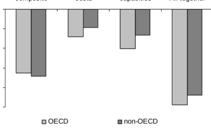
(14) 14 OECD countries respectively. Cheaper carbon-free technologies foster a faster penetration of these techniques and thus reduce the tax impact on electricity prices and partly the crowding-out effect, but the gain from this more optimistic assumption is inhibited by the pace of replacement of production capacities. A good indicator of this inertia effect is the carbon content of the composite goods displayed in Table 5 for various stabilization targets. Although the carbon content of new equipments start declining as soon as 2005 and is drastically cut down in 2100 (between 80% and 95% for 550 ppm with ITC) it is remarkable that the average carbon content of the production of the composite good is still very high in 2050. At that date the equipment stocks is still composed of equipments build in 2020 (for the electric sector). This generates an obvious environmental irreversibility: given the cumulated carbon release in the first periods, the abatement requirements to meet the carbon targets have to increase sharply by the second part of the century. Scenarios 2050 2100 550 ppm with ITC (tax =1.5) -29% -56% 450 ppm with ITC (tax =3.8) -47% -78% 550 ppm without ITC (tax =4) -33% -61% 450 ppm without ITC (tax =12.15) -51% -83% Table 5: variations in the carbon content of composite goods (w.r.t. the reference scenario). diminution of total discounted costs. The impact of this barrier is fully demonstrated by reducing the lifetime of productive capacity in the electric sector by 20%: this allows for 10.0% and 6.7% reductions of the consumption losses in OECD and non-OECD respectively. Thanks to lower inertia, equipments purchased in the first decades of the century (most of them installed in the DCs) are retired more quickly when carbon prices go up, thus reducing the environmental irreversibility effect. Finally the joint effect of technological optimism and lower inertia will allow fot cutting by 24.5% and 22% total consumption losses for OECD and non-OECD respectively.. +20% EE composite. 20% faster decrease of investment costs. -20% Lifetime electric capacities. All together. 0.00% -5.00% -10.00% -15.00% -20.00% -25.00% OECD. non-OECD. Figure 2 : Impact of 20% changes in technical parameters.

(15) 15. 5.2. Beyond carbon price only policies, a broader view of structural change. The slowness in curbing down carbon emissions is far more impressive in the transportation sector since, in the absence of a carbon free backstop substitute but with significant efficiency improvements, neither for the 550 ppm nor for the 450 ppm target does the assumption of ITC lead to reductions in emissions from transportation (see Table 2). This is typically the type of phenomenon that IMACLIM-R is designed to reveal and explain, and which forces to consider the role of induced structural change. Let us first examine issues related to freight dynamics. The above simulations considered that the transportation content of the production of the composite good was sensitive to the transportation prices. But the development of freight ultimately depends on the localization patterns of production and consumption, themselves depending on a multiplicity of factors beyond transportation costs such as international wages discrepancies, industrial specialization and trade-offs between supply security and minimizing stocks through ‘just on time’ production. No information is currently available about how drastic carbon policies would impact on these parameters. To give the order of magnitude of the stake, we considered that non-price determinants may offset the impact of higher transportation prices, so that the ‘freight content’ of production remains constant. This single modification suffices in increasing the discounted losses for 550 ppm with ITC from 1.1% to 3%. Without any pretention to realism, this simulation points out a key mechanism of a more general interest: even though the share of transportation in total costs is low, keeping constant the corresponding i/o coefficients causes a very high increase in mitigation costs, due to the fact that once exhausted the bulk of carbon-saving potentials in transportation, constraining carbon emissions mechanically amounts to constraining economic growth. This is a typical illustration of the interest of an extended dialogue where top-down analysis helps detecting issues which are still underworked by sector-based analysis. Let us now pass to the question of the mobility demand. IMACLIM-R accounts for the fact that the development of infrastructures induces additional demand, as it increases the time- and cost-efficiency of transportation. In our central case, decisions to build new infrastructures rest on the same rationale as for any other production capacities: when infrastructures approache saturation, it enhances their expected profitability and triggers investments to expand the network. This in turn reinforces the modal shares of road and air transportation21. However, infrastructure decisions are, under forms that vary in function of their institutional context, a case of private-public partnership in which local authorities give authorizations and subsidies to private and public agents, subject to constraints on pricing and project specifics. Public authorities, with interests other than energy and climate goals, also influence transportation investments indirectly through urban and land-use policies. For example, real estate pricing and loan practices are just as important signals as gasoline prices for determining the localization choices of households22. This may lead to transportation policies driven by the combination of many public concerns and supported by a wider set of policy instruments than carbon prices. We illustrate them in an aggregated way through a simple decision routine of limiting investments in road infrastructures at a maximum ceiling. 21. A ex post check on transportation trends show that we produce trends with the same order of magnitude as scenarios of (WBCSD, 2004) and (Schäffer et Victor, 2000). 22 For example in France the evolution of average prices of fuels (gasoline, unleaded gasoline, diesel) since 1960 does not statistically present a significant upward trend, whereas the price of real estate were multiplied by a factor 3..

(16) 16 This has a significant impact on emissions and, for a stabilization at 550 ppm under ITC, the required level of the yearly tax increment is $1.2 per ton of carbon with the alternative complementary infrastructure policy instead of $1.5 with ‘carbon price only’ policy (Figure 3)23. Combined with a limitation of investments in both transportation and energy infrastructures, this results in a 2.4% total discounted consumption gain instead of a -1.1% loss. ETC. ETC + transport infrastructure policy. 450 ppm. ATC. 550 ppm. Annual tax increment from 2005 to 2100. 12. 10. 8. 6. 4. 2. 0 500. 550. 600. 650. 700. 750. 800. 850. 900. 950. 1000. Carbon budget 2000-2100 (GtC). Figure 3: tax-constrained carbon budget under various assumptions This result demonstrates the interest of accounting for induced changes in households’ demand as one of the driver of overall structural change, and of not letting the sole carbon price the charge of curbing down emissions from transportation. To go beyond this preliminary exercise would imply to incorporate analysis developed in the field of urban economics (Fujita, 1991) about the dynamics of lifestyles choice and localization patterns, and to describe better interactions between land-use patterns and the price of real estate. 6. Conclusion. Advocates of modeling technical change as induced by economic signals (Grubb, 1997) and not purely as an exogenous process argue that, by taking into account the induced accelerated innovation process and penetration of new techniques, models using this approach yield a more realistic representation of costs of mitigation policies. This paper does not pretend to establish what is realistic and what is not. Rather the above comparative exercise demonstrates that adopting an endogenous framework induces additional complexities, which blurs an univocal view of ITC causing lower policy costs and suggests that this causality requires a broader view of policy instruments. First, we confirm the intuition that the overall effect of ITC mechanims is to lower stabilization costs thanks to the gain from larger efficiency improvements and faster penetration of carbon free techniques, which gains are not offset by the crowding-out of non-energy investments. The increased energy bill hampers on sector profitability and. 23. In the 450 ppm case, the tax increment falls from $3.8 down to $3.0.

(17) 17 constrains households budget, and the induced technical change reduces more quickly the impact on these two parameters. Second, sensitivity tests all corroborate the critical role of the interplay between the carbon tax, the pace of technical progress on low-carbon technologies and the pace of turnover of equipments. The role of inertia in the diffusion of carbon-intensive production techniques is magnified in our simulations: (i) the carbon taxes start low, increases linearly and do not exert a strong incentive to decarbonization in the first decades; (ii) imperfect foresight of investors about future tax profiles makes them continue to build equipment stocks with a non-optimal carbon intensity. This suggests that a major way of reducing stabilization costs is to launch credible signals to stabilize the expectations of decisionmakers and to examinate futher the optimal time profile of carbon prices under ITC (benefits of accelerated technical change vs. costs of accelerated scrapping of capital stock). Third, the role of inertia is aggravated by the rebound effect of energy efficiency in the transportation sector and by the induction of mobility demand that offsets part of the efficiency gains. Infrastructures built in the following decades will induce carbon intensive consumption patterns that are hard to reverse. This is all the more critical in developing countries which will build the bulk of these infrastructures in the following decades; there is a danger of a lock-in on carbon intensive development patterns that is hard to unlock overnight. Fourth, the assumption of induced technical change makes the policy context far more complex; it forces to diversify policy signals in order to change some key parameters of the economic growth engine.Beyond the role of R&D policies, it shows the importance of infrastructure policies, of policies affecting the pace of capital stock turnover and of the prices of the real estates. Finally, in spite of the current limits of our modeling framework, we hope to have demonstrated the interest and the possibility of modeling technical change not only as ‘pure’ efficiency gains on carbon saving techniques but also as a process of induction of consumption pattern and structural change.. 7. References. Ambrosi P., J.C. Hourcade, S. Hallegatte, F. Lecocq, P. Dumas, M. Ha Duong (2003), “Optimal control models and elicitation of attitudes towards climate damages”, Environmental Modeling and Assessment 8(3): 133-147. Armington, P. S. (1969). "A Theory of Demand for Products Distinguished by Place of Production." IMF, International Monetary Fund Staff Papers 16: 170-201. Blanchflower, D. G. and A. J. Oswald (1995). "An introduction to the Wage Curve." Journal of Economic Perspectives 9(3): 153-167. Barro R. J. and X. Sala-i-Martin, (1998) . Economic Growth, MIT Press. Crassous, R., J.-C. Hourcade and O. Sassi (2005). “IMACLIM-R: a modeling framework of sustainable development issues”. International Workshop on Hybrid Energy-Economy Modeling, Paris, 20-21st April 2005..

(18) 18. Fujita, M. (1991). Urban Economic Theory. Land-use and City Size, Cambridge University Press, March 1991, 378 p. Ghersi, F., J.-C. Hourcade and P. Criqui (2003). “Viable Responses to the EquityResponsibility Dilemma: a Consequentialist View”. Climate Policy 3(1):115-133 Grubb, M. (1997). “Technologies, energy systems and the timing of CO2 abatement. An overview of economic issues”, Energy Policy 25(2):159-172. Hourcade, J.C. (1993). “Modeling long-run scenarios. Methodology lessons from a prospective study on a low CO2 intensive country”. Energy Policy 21(3): 309-326. IPCC Special Report on Emissions Scenarios (SRES), N. Nakicenovic, J. Alcamo, G. Davis, B. de Vries, J. Fenhann, S. Gaffin, K. Gregory, A. Grübler, et al., (2000). Special Report on Emissions Scenarios, Working Group III, Intergovernmental Panel on Climate Change (IPCC), Cambridge University Press, Cambridge, 595 pp. http://www.grida.no/climate/ipcc/emission/index.htm IPCC, B. Metz, O. Davidson, R. Swart, J. Pan (eds.) (2001). Climate Change 2001: Mitigation. Contribution of Working Group III to the Third Assessment Report of the Intergovernmental Panel on Climate Change, UNEP, WMO, Cambridge University Press. Lecocq, F., J.C. Hourcade and M. Ha-Duong (1998). “Decision making under uncertainty and inertia constraints : sectoral implications of the when flexibility”. Energy Economics 20(5/6): 539-555. Maddison, A. (1995). Monitoring the world economy: 1820 – 1992, OECD Development Center, August 1995, 260 p. Oliveira Martins, J., F. Gonand, P. Antolin, C. de la Maisonneuve, and Kwang-Y (2005). "The impact of ageing on demand, factor markets and growth”, OECD Economics Department Working Papers, #420, OECD Economics Department Schäfer, A. and D.G. Victor (2000). “The future mobility of future population”, Transportation Research Part A 34:171-205. Smulders, S. and M. de Nooij (2003). “The impact of energy conservation on technology and economic growth”. Resource and Energy Economics 25: 59-79. Solow, R. (1990) “Reactions to Conference Papers” in Diamond, P. (ed.), Growth, Productivity, Unemployment: Essays to Celebrate Bob Solow’s Birthday, The MIT Press. WBCSD (World Business Council for Sustainable Development) (2004). “Mobility 2030: meeting the challenges to sustainability”, Final report 2004. http://www.wbcsd.ch/web/publications/mobility/mobility-full.pdf Wright, G. (1990). "The Origins of American Industrial Success, 1879-1940," American Economic Review 80(4): 651-68. Zahavi, Y. and A. Talvitie (1980). “Regularities in travel time and money expenditures”. Transportation Research Record 750, 13±19..

(19) 19 Appendix A: Productivity, Population and Real GDP Growth in the Baseline Scenario. OECD 3%. 2%. 1%. 0% 1990. 2010. productivity. 2030. 2050. 2070. 2090. productivity + population. 2110. real GDP. ASIA 6%. 4%. 2%. 0% 1990. 2010. productivity. 2030. 2050. 2070. 2090. 2110. real GDP. productivity + population. REF 6%. 4%. 2%. 0% 1990. 2010. productivity. 2030. 2050. 2070. productivity + population. 2090. 2110. real GDP.

(20) 20. ALM 4%. 3%. 2%. 1%. 0% 1990. 2010. 2030. productivity. 2050. 2070. 2090. productivity + population. 2110. real GDP. OPEC 3%. 2%. 1%. 0% 1990. 2010. productivity. 2030. 2050. 2070. productivity + population. 2090. 2110. real GDP.

(21) 21. Appendix B: Key Indicators of Development Pathways Annual growth rates. Levels. Final consumption of composite goods ($1997 per capita). Final consumption of energy (toe per capita). Share of fossil fuels in final energy consumption. Stock of building (m² per capita). Stock of cars per capita. Oil world price. 2000. 2050. 2100. 20002050. 20502100. OECD. 8450. 20257. 32811. 1.76%. 0.97%. Non-OECD. 307. 944. 1701. 2.27%. 1.18%. ASIA. 192. 752. 1226. 2.77%. 0.98%. REF. 438. 3317. 6107. 4.13%. 1.23%. ALM. 470. 852. 1633. 1.20%. 1.31%. OPEC. 534. 1207. 2695. 1.64%. 1.62%. OECD. 1.021. 1.561. 1.624. 0.85%. 0.08%. non-OECD. 0.132. 0.392. 0.410. 2.20%. 0.09%. ASIA. 0.094. 0.377. 0.347. 2.81%. 0.17%. REF. 0.418. 1.453. 2.004. 2.52%. 0.64%. ALM. 0.095. 0.180. 0.181. 1.29%. 0.01%. OPEC. 0.276. 0.785. 1.152. 2.11%. 0.77%. OECD. 84%. 87%. 73%. Ò. Ô. Non-OECD. 85%. 94%. 84%. Ò. Ô. ASIA. 81%. 81%. 70%. -. Ô. REF. 88%. 92%. 88%. Ò. Ô. Ò. Ô. ALM. 85%. 90%. 83%. OPEC. 86%. 92%. 83%. Ò. Ô. OECD. 40. 59. 98. 0.79%. 1.02%. non-OECD. 10. 17. 39. 1.07%. 1.64%. ASIA. 8. 14. 34. 1.00%. 1.78%. REF. 13. 31. 74. 1.70%. 1.77%. ALM. 11. 18. 37. 0.91%. 1.44%. OPEC. 14. 27. 59. 1.29%. 1.56%. OECD. 0.40. 0.55. 0.73. 0.66%. 0.56%. non-OECD. 0.03. 0.10. 0.19. 2.50%. 1.34%. ASIA. 0.01. 0.08. 0.17. 4.20%. 1.37%. REF. 0.11. 0.34. 0.71. 2.26%. 1.46%. ALM. 0.04. 0.09. 0.17. 1.41%. 1.32%. OPEC. 0.03. 0.08. 0.18. 2.26%. 1.55%. world. 118. 132. 426. 0.22%. 2.36%. Coal. -38. -121. -206. -. -. Oil. -1032. -3227. -3259. -. -. Gaz. -157. -454. -1065. -. -. Et Elec. -80 -1. -47 -30. 120 -38. -. -. OECD composite net flow (billions $1997). 966 160. 2 476 600. 4 219 200. -. -. OECD Net Capital Flows Exp (-) Imp (+) (billions $1997). -29200. -98000. -44000. -. -. OECD Energy net flows Exp (+) Imp (-). (Mtoe).

(22) 22 Appendix C:. Energy - Growth decoupling: the role of structural effects 1.1 1 0.9 0.8 0.7 0.6 0.5 0.4 0.3 2000. 2020. 2040. OECD total decoupling ASIA total decoupling REF total decoupling ALM&OPEC total decoupling. 2060. 2080. OECD structural effect ASIA structural effect REF structural effect ALM&OPEC structural effect. 2100.

(23)

No results found