del Servizio Studi
Risk aversion, wealth and background risk
by Luigi Guiso and Monica Paiella
gerimenti.
I lavori pubblicati nella serie riflettono esclusivamente le opinioni degli autori e non impegnano la responsabilità dell’Istituto.
Comitato di redazione:
STEFANO SIVIERO, EMILIA BONACCORSIDI PATTI, MATTEO BUGAMELLI, FABIO BUSETTI, FABIO FOR -NARI, RAFFAELA GIORDANO, MONICA PAIELLA, FRANCESCO PATERNÒ, ALFONSO ROSOLIA, RAFFAELA BISCEGLIA (segretaria)
Abstract
We use household survey data to construct a direct measure of absolute risk aversion based on the maximum price a consumer is willing to pay to buy a risky security. We relate this measure to consumers’ endowment and attributes and to measures of background risk and liquidity constraints. We ¿nd that risk aversion is a decreasing function of endowment -thus rejecting CARA preferences - but the elasticity to consumption is far below the unitary value predicted by the CRRA utility. We also ¿nd that households’ attributes are of little help in predicting their degree of risk aversion, which is characterized by massive unexplained heterogeneity. However, the consumers’ environment affects risk aversion. Individuals who are more likely to face income uncertainty or to become liquidity constrained exhibit a higher degree of absolute risk aversion, consistent with recent theories of attitudes towards risk in the presence of uninsurable risks.
JEL Classi¿cation: D10, D80.
Keywords: heterogeneous preferences, risk tolerance, background risk, liquidity constraints.
Contents
1. Introduction . . . 7
2. Measuring risk aversion . . . 9
2.1 Risk aversion with background risk . . . 12
3. Descriptive evidence . . . 13
4. Empirical speci¿cation . . . 16
5. Results . . . 18
6. Robustness . . . 21
6.1 Endogenous consumption and wealth . . . 21
6.2 Quantile regressions . . . 23
7. Risk aversion and background risk . . . 24
8. Consistency with observed behavior . . . 26
8.1 Wealth-portfolio relation . . . 27
8.2 Age-portfolio pro¿le. . . 27
8.3 Euler equation estimates . . . 28
9. Conclusions . . . 30
Tables and¿gures . . . 33
Appendix . . . 40
References . . . 46
* Università degli studi di Sassari and Ente Einaudi. ** Bank of Italy, Economic Research Department.
the degree of absolute risk aversion or of absolute risk tolerance, and wealth is central to many
¿elds of economics. Kenneth Arrow argued as long as 35 years ago that “the behavior of these
measures as wealth varies is of the greatest importance for prediction of economic reactions in the presence of uncertainty” (p. 35).
Most of the inference on the nature of this relation is based on common sense, introspection, casual observation of behavioral differences between the rich and the poor and a priori reasoning, and concerns the sign of the relation, whereas no evidence at all, even indirect, is available on its curvature. The consensus view is that absolute risk aversion should decline with wealth.2 Furthermore, if one agrees that preferences are characterized by constant
relative risk aversion - a property of one of the most commonly used utility functions, the isoelastic - then absolute risk aversion is decreasing and convex in wealth, while risk tolerance is increasing and linear. The curvature of absolute risk tolerance has been shown to be relevant in a number of contexts. For instance, Gollier and Zeckhauser (1997) show that it determines whether the portfolio share invested in risky assets increases or decreases over the consumer life cycle, an issue that is receiving increasing attention. Moreover, if risk tolerance is concave, wealth inequality can help elucidate the risk premium puzzle (Gollier, 2001a). Furthermore, the curvature of risk tolerance and the nature of risk aversion may explain why the marginal propensity to consume out of current resources, rather than being constant, declines as the level of resources increases (Carroll and Kimball, 1996, and Gollier, 2001b).
4 We thank Chris Carroll, Christian Gollier, Michaelis Haliassos, Wilko Letterie, Winfried Koeniger, John
Pratt, Andrea Tiseno and Richard Zeckhauser for very valuable discussion and suggestions. We are also greateful to participants at seminars at Birbeck College, City University London, European University Institute, University of Leuven, Ente Luigi Einaudi lunch seminars, Rand Corporation, Universidad Carlos III, the TMR conference “Savings, pensions, and portfolio choice”, Deidesheim, the NBER 2000 Summer institute “Aggregate implica-tions of microeconomic consumption behavior”, the 27th EGRIE meeting for helpful comments. Luigi Guiso acknowledges¿nancial support from MURST, and the EEC for the TMR research project “Specialisation versus diversi¿cation: the Microeconomics of Regional Development and the Spatial Propagation of Shocks in Europe”. Cristiana Rampazzi provided excellent research assistantship. Only the authors are responsible for the contents of this paper which does not reÀect the Community’s opinion, nor the Bank of Italy’s.
5 It is on these grounds that quadratic and exponential utility, though often analytically convenient, are
regarded as misleading representations of preferences the ¿rst implies increasing absolute risk aversion while the second posits it is constant.
The aim of this paper is to provide empirical evidence on the nature of the relationship between risk aversion and wealth. Using data from the Bank of Italy Survey of Household Income and Wealth (SHIW), we employ the information on household willingness to pay for a risky security to recover a measure of the Arrow-Pratt index of absolute risk aversion of the consumer lifetime utility function and relate it to indicators of consumers’ endowment, as well as to a set of demographic characteristics to control for individual preference heterogeneity.
The usual de¿nition of risk aversion and tolerance developed by Arrow (1970) and Pratt (1964) is based on the assumption that initial wealth is non-random. It is also constructed in a static setting or in settings where full access to the credit market is assumed. Recently, it has been shown that attitudes towards risk can be affected by the prospect of being liquidity-constrained and by the presence of additional uninsurable, non-diversi¿able risks. Gollier (2000b) shows that the possibility that consumers will be subject to a liquidity constraint in the future makes them less willing to bear risk presently, i.e. increases their risk aversion. Pratt and Zeckhauser (1987), Kimball (1993) and Eekhoudt, Gollier and Schlesinger (1996) establish a set of conditions on preferences that de¿ne classes of utility functions whose common feature is that the presence of background risk makes the individual behave in a more risk-averse manner. They call these classes of utility functions “proper”, “standard” and “risk vulnerable”, respectively.3 The main implication is that even if risks are independent, individuals will react
to background risk by reducing their exposure to avoidable risks. One important consequence is that individuals facing high exogenous labor income risk - which is normally uninsurable - will be more risk-averse and thus avoid exposure to portfolio risk by holding less or no risky assets. Similarly, they tend to buy more insurance against the risks that are insurable (Eekhoudt and Kimball, 1992).4 Furthermore, insofar as income risk evolves with age, under
standardness, background risk may help explain the life cycle of asset holdings. Several papers
6 Pratt and Zeckhauser (1987) de¿ne as “proper” the class of utility functions that ensure that introducing an
additional independent undesirable risk when another undesirable one is already present makes the consumer less willing to accept the extra risk. Kimball (1993) de¿nes as “standard” the class of utility functions that guarantee that an additional independent undesirable risk increases the sensitivity to other loss-aggravating ones. Starting from initial wealthz, a risk h{ is undesirable if and only if it satis¿es Hx+z h{, x+z,, where x+z, is an increavlqg and concave utility function. A risk h{ is loss-aggravating if and only if it satis¿es Hx3+z . h{, x3+z, . When absolute risk aversion is decreasing, every undesirable risk is aggravating, but not every
loss-aggravating risk is undesirable. Finally, risk vulnerability in Eeckhoudt, Gollier and Schlesinger (1996) implies that adding a zero-mean background risk makes consumers more risk averse.
7 Guiso, Jappelli and Terlizzese (1996)¿nd that households facing greater earnings risk buy less risky assets
have cited background risk and risk vulnerability (or standardness) to explain the portfolio puzzles.5 In all these studies, standardness or risk vulnerability is just assumed, but it is not
tested because of lack of evidence on individual risk aversion.
The evidence presented in this paper also sheds light on the empirical relevance of these concepts. The availability of information on measures of background risk and on proxies of borrowing constraints allows us to relate our index of risk aversion to indicators of income-related risk and of liquidity constraints.
Our¿ndings show that absolute risk tolerance is an increasing and concave function of consumers’ resources: thus, we reject both CARA and CRRA preferences. Furthermore, we
¿nd that risk aversion is positively affected by background risk, as well as by the possibility of
being credit constrained. Our estimates, however, show that these variables can only explain a small amount of the sample variability in attitudes towards risk. Even after controlling for individual characteristics there remains a large amount of unexplained variation reÀecting partly genuine differences in tastes.
The rest of the paper is organized as follows. Section 2 describes our measure of risk aversion when wealth is non-random and when there is background risk. Section 3 presents descriptive evidence on absolute risk aversion in our cross-section of households. In Section 4 we discuss the empirical speci¿cation we use to relate absolute risk aversion to the consumer endowment, attributes and then environment. Section 5 presents the results of the estimates. In Section 6 we check the robustness of the main¿ndings to the endogeneity of consumption and wealth, non-responses and the possible presence of outliers. Section 7 presents evidence regarding the effects of background risk on the propensity to bear risk. Section 8 discusses the consistency with observed behavior of our ¿ndings on the shape of the wealth-risk aversion relation. Section 9 summarizes and concludes.
2. Measuring risk aversion
To measure absolute risk aversion and tolerance we exploit the 1995 wave of the Survey of Household Income and Wealth (SHIW), which is run biannually by the Bank of Italy. The 1995 SHIW collects data on income, consumption, real and ¿nancial wealth, and on several
8 See Weil (1992), Gollier and Zeckhauser (1997), Gollier (2000), Coco et al. (1998), Heaton and Lucas
demographic variables for a representative sample of 8,135 Italian households. Balance-sheet items are end-of-period values. Income andÀow variables refer to 1995.6
The 1995 wave has a section designed to elicit attitudes towards risk. Each participant is offered a hypothetical security and is asked to report the maximum price that he would be willing to pay for it. Speci¿cally:
“We would like to ask you a hypothetical question that you should answer as if the situation were a real one. You are offered the opportunity of acquiring a security permitting you, with the same probability, either to gain 10 million lire or to lose all the capital invested. What is the most that you would be prepared to pay for this security?”
Ten million lire is equal to just over 5,000 euros (or roughly $5,000). The ratio of the expected gain from the investment to average household total consumption is 16 percent thus, the investment represents a relatively large risk. We consider this to be an advantage since expected utility maximizers behave as risk-neutral individuals with respect to small risks even if they are risk-averse to larger risks (Arrow, 1970). Thus, putting consumers face to face with a relatively large investment is a better strategy to elicit risk attitudes when one relies, as we do, on expected utility maximization to characterize risk aversion.7 The interviews
are conducted personally at the consumer’s home by professional interviewers. To help the respondent understand the question, the interviewers show an illustrative card and are ready to provide explanations. The respondent can answer in one of three ways: a) declare the maximum amount he is willing to pay for the security, which we denote~ b) answer “don’t
know” c) not answer.
Notice that the way the hypothetical security is designed implies that with probability 1/2 the respondent gets 10 million lire and with probability 1/2 he loses~ So the expected value
of the lottery is*2Ef ~ Clearly, ~ f million lire, ~ =f, and ~ : f million lire
imply risk aversion, risk neutrality and risk loving, respectively. This characterizes attitudes
9 See the appendix for a detailed description of the survey contents, its sample design, interviewing
proce-dure and response rates.
: In this vein, Rabin (2000) argues that if an expected utility maximizer refuses a small risk at all levels
of wealth then he must clearly exhibit unrealistic levels of risk aversion when faced with large-scale risks. This again suggests that offering large investments is a better way to characterize the risk aversion of expected utility maximizers.
towards risk qualitatively. But we can do more within the expected utility framework a measure of the Arrow-Pratt index of absolute risk aversion can be obtained for each consumer. Let denote household r endowment, which for a moment is assumed to be non-random. Let E be its (lifetime) utility function and h be the random return on the security for individual, taking values 10 million and ~ with equal probability. The maximum purchase price is thus given by:
E ' 2En f n 2E ~ ' .En hc
(1)
where . is the expectations operator. Taking a second-order Taylor expansion of the right-hand side of (1) aroundgives:
.En h f E n E.E h n fDE.E h2
(2)
Substituting (2) into (1) and simplifying we obtain:
-E f E*E ' eED ~*2*f2n ~2
(3)
Equation (3) uniquely de¿nes the Arrow-Pratt measure of absolute risk aversion in terms of the parameters of the hypothetical security of the survey. Absolute risk tolerance is de¿ned byAE ' *-E. Obviously, for risk-neutral individuals (i.e. those reporting ~ ' f),
-E ' f and for the risk-prone (those with ~ : f), -E f. According to (3) absolute
risk aversion may vary with consumer endowment and with all the attributes correlated with his preferences. Notice that since the loss ~ or the gain from the investment need not be fully borne by or bene¿t current consumption but may be spread over lifetime consumption, our measure of risk aversion is better interpreted as the risk aversion of the consumer lifetime utility and as his lifetime wealth.8
A few comments on this measure and on how it compares with those used in other studies are in order. First, our measure requires no assumption on the form of the individual utility function, which is left unspeci¿ed. Second, it is not restricted to risk-averse individuals
; Tiseno (2002) studies the relationship between the risk aversion of lifetime utility and that of period utility
and shows how one can recover the latter given information on the curvature of the former and on the slope of the consumption function. He also shows that knowledge of the maximum subjective price function for a risk is suf¿cient to identify the risk aversion of a consumer lifetime utility.
but extends to the risk-neutral and the risk lovers. Third, our de¿nition provides a point estimate, rather than a range, of the degree of risk aversion for each individual in the sample. These features distinguish our study from that of Barsky, Juster, Kimball and Shapiro (1997) who only obtain a range measure of (relative) risk aversion and a point estimate under the assumption that preferences are strictly risk-averse and utility is of the CRRA type. More, their sample consists of individuals aged 50 or over, which makes it hard not only to study the age pro¿le of risk aversion but also to test its relationship with background risk since this is likely to matter most for the young. The study of this relationship is instead one of the aims of our paper. However, their elicitation strategy allows them to recover a measure of the risk aversion of period utility instead of lifetime utility as we do. In this regard, our and their study should be viewed as complementary.9
2.1 Risk aversion with background risk
The measure of risk aversion in (3) is for non-random endowment, but it is easily generalized to the case of background risk using the results of Kihlstrom, Romer and Williams (1981) and Kimball (1993). For this purpose we have to restrict the analysis to risk-averse individuals (i.e. those reporting~ f).
Let h+ denote a zero-mean background risk for individual , whose variance is j2. Denoting with .% E% ' +c ) the expectation with respect to the random variable h%, our
indifference condition for purchasing the risky security and paying~ becomes
.+En h+ ' ..+En h+n hc
(4)
where we have implicitly assumed that the background risk and the risky security are independent, which is assured by construction. If preferences are risk-vulnerable as in Gollier and Pratt (1996), we can use the equivalence:
.+En h+ ' Ec
(5)
< The Barsky et al. (1997) measure of risk aversion has other advantages. Since the risk tolerance question
is asked in two waves of the survey they use and a subset of the respondents is common to both waves, they can account for measurement errors in their measure of relative risk aversion. Furthermore, they collect information on intertemporal substitution and can thus study its relation to risk aversion.
whereE is a concave transformation of , which implies thatE is more risk-averse
than E. In other words, if consumers and are both risk-averse and their preferences are risk-vulnerable, then, assuming ' , is more risk-averse than if h+ is riskier than h+, i.e. if the background risk is greater.
We can thus account for background risk by expressing our measure of risk aversion in terms of the utility functionE to get
-E f E*E ' eED ~*2*f2n ~2
(6)
Risk aversion will now vary not only with the consumer’s endowment and attributes but also with any source of uncertainty characterizing the environment. If measures of the latter are available, one can directly test for standardness of preferences.
Interestingly, the shape of the relation between - (or risk tolerance) and can have implications for the sign of the effect of background risk on absolute risk aversion. Hennessy and Lapan (1998) show that a positive and concave relation of risk tolerance with wealth is suf¿cient for preferences to be standard as in Kimball (1993). Similarly, Eekhoudt, Gollier, and Schlesinger (1996) show that a suf¿cient (but not necessary) condition for absolute risk aversion to increase with background risk is that it should be a decreasing and convex function of the endowment, an assumption that is satis¿ed, for instance, by the CRRA utility. Gollier and Pratt (1996) argue that the convexity of absolute risk aversion should be regarded as a natural assumption10
, “since it means that the wealthier an agent is, the smaller is the reduction in risk premium of a small risk for a given increase in wealth”. Though plausible, this assertion is not backed by any empirical evidence. Our results lend support to this conjecture in that they imply that absolute risk aversion is a convex function of the endowment. In Section 4, we will discuss the implications for the relation between risk aversion ofE and the level of endowment from the relation between the risk aversion ofE and the endowment.
3. Descriptive evidence
The question on the risky security was submitted to the whole sample of 8,135 heads of household, but only 3,458 answered and were willing to purchase the security. Out of the
43 Notice that if consumers are risk-averse at all levels of wealth and if absolute risk aversion is a strictly
4,677 who did not, 1,586 answered “do not know” and 3,091 refused to answer or to pay a positive price (25 offered more than 20 million). This is likely to be due to the complexity of the question, which might have led some participants to skip it altogether because of the relatively long time required to understand its meaning and provide an answer. Non-responses are also a reÀection of the fact that the question on the risky security was asked abruptly by the interviewers, without preparing the respondents with a set of “warm up” questions. However, this strategy has its advantages: ¿rst, depending on how the introductory questions are framed and when they are asked, they may end up affecting the answers, thus distorting the measure of the true preference parameter this is avoided by asking the question abruptly. Second, it avoids bringing in noisy respondents (e.g. those with a poor understanding of the question), as would probably happen with “warm up” questions. Thus, while a high non-response rate signals that the question is complex and there may be cognitive problems, it does not mean that those who chose to respond gave erroneous answers. On the contrary, if those who answered did so because they had a good understanding of the question (or the time to grasp and answer it), the elicitation strategy with no “warm up” questions might have been an effective way to get rid of noisy respondents.
One way to assess whether the risk-aversion measure reÀects just noise or reveals instead the risk attitudes of the individual, is to check whether it has predictive power over consumer choices that theory predicts should be affected by individuals’ risk aversion. Guiso and Paiella (2001) show that our survey measure of risk aversion has considerable predictive power of such behaviors as occupation choice, risky asset ownership and portfolio allocation, willingness to move and change job, as well as health status, in ways that are consistent with what the theory predicts. On the basis of probit regressions with standard socio-economic controls, the risk-averse turn out to be signi¿cantly less likely to be self-employed, are somewhat more likely to be public employees and are less likely to change job than the risk-neutral and risk lovers. Further, the probability of holding risky assets, i.e. private bonds, stocks and mutual funds, is less than half as great among averse consumers than among the neutral and risk-lovers. Based on this evidence we feel con¿dent that despite the extent of non-responses, the risk attitude indicator captures the individual willingness of the respondents to bear risk.11
44 This is not to say that our measure of risk aversion is free of measurement error. However, if this is of the
Table 1 reports descriptive statistics for the whole sample of 8,135 households, for the sample of 3,458 respondents to the risky security question and, for the latter, for several sub-samples. Out of 3,458 individuals willing to purchase the security the great majority (96 percent) are risk averse, in that they report a maximum price lower than the gain offered by the security 144 individuals are either risk-neutral (125, or 3.6 percent of the sample), or risk-lover (19, only a tiny minority). The table reports characteristics for these three sub-samples too. Those who responded to the question are on average 6 years younger than the total sample and have higher shares of male-headed households (79.8 compared to 74.4 percent), of married people (78.9 and 72.5 percent, respectively), of self-employed (17.9 and 14.2 percent) and of public sector employees (27.5 and 23.3 percent, respectively). They are also somewhat wealthier and slightly better educated (1.3 more years of schooling). These differences seem to suggest that there are some systematic effects explaining the willingness to respond. Probit regressions, reported in the Appendix (column (1) and (2) of the table), con¿rm this factual evidence and suggest that the probability of answering the question is higher among younger and more educated households. Public employees and the self-employed are also relatively more likely to respond. Further, the response probability increases in household income, but decreases with net worth. In our estimates we control for the possibility that non-responses induce selection bias.
The sub-samples of risk-lovers and risk-neutral, on the one hand, and risk-averse consumers, on the other, exhibit several interesting differences. The risk-averse are younger and less educated they are less likely to be male, to be married and to live in the North of Italy. Strong differences also emerge comparing the type of occupation: among the risk-averse the share of self-employed is 17.4 percent among the risk-prone or risk-neutral it is much higher at 29.2 percent. This ordering is reversed for public sector employees. The lovers and risk-neutral are public employees in 27 percent of cases, while the risk-averse in 28 percent. These differences are likely to reÀect self-selection, with more risk-averse individuals choosing safer jobs. Finally, notice that the risk-averse are signi¿cantly less wealthy than the risk-lovers or risk-neutral (170 million lire - 88,000 euros - of median net worth compared with 330 million - 170,000 euros).
Table 1 also reports the characteristics of the moderately risk-averse consumers (at or below the sample median of the reported price~) and of the high risk-averse (above median).
Highly risk-averse consumers are on average two years older, somewhat less well educated, less likely to be married and much more likely to live in the South. They are also less wealthy than the moderately risk-averse, both in terms of net worth,¿nancial wealth and consumption (the median net worth of the two groups is 154.9 and 198.5 million lire, respectively). Finally, the share of self-employed is 15.6 percent for the highly risk-averse and 20.1 percent for the moderately risk averse that of public sector employees is 28.3 and 26.3 percent. Thus, being risk-averse as opposed to risk-lover or risk-neutral, as well as differences in the degree of risk aversion seem to explain sorting into riskier occupations.
4. Empirical speci¿cation
Most of the literature assumes that agents are risk-averse and is interested in assessing how risk aversion varies with the consumer’s attributes and in particular with his endowment. Accordingly, the next four sections focus on risk-averse individuals.
To estimate the relation between our index of absolute risk aversion and the individual endowment we use the following speci¿cation (we omit the household index for brevity):
-E ' @eMn#
q '
V qc
(7)
where denotes the (lifetime) endowment, M is a vector of consumer characteristics affecting individual preferences,# is a random shock to preferences, @ is a constant and and q are two unknown parameters.12 Equation (7) is a generalization of absolute risk aversion under CRRA
preferences the latter obtain when q = 1 in which case V ' @eMn# measures relative risk aversion. Notice that-E is always positive and is decreasing in for all positive values of q. Furthermore, ifq : 0, it is always convex in . Though simple, this formulation is Àexible enough to allow us to analyze the curvature of absolute risk tolerance, which is de¿ned as:
AE ' V3q
(8)
Thus, ifq : 0, risk tolerance is an increasing function of furthermore, it will be concave, linear or convex in depending on whether q is less than, equal to or greater than 1. Since
45 Notice that our empirical speci¿cation (7) does not allow for heterogeneity in the parameter. If varies
across individuals our estimates would be affected by heteroschedasticity. However, a formal test cannot reject the null hypothesis that the error term is homoschedastic.
q measures the speed at which -E declines with endowment, AE is a concave (respectively
convex) function of if absolute risk aversion falls as consumption increases more slowly (respectively faster) than that characterizing CRRA preferences. Since most theoretical ambiguities rest on the curvature ofA, not -, our approach is not restrictive.
Although equation (7) is assumed, a utility function that gives rise to a measure of absolute risk aversion as in (7) is
E ' ]
e3 @eMn# h3q3q_ h '] e3 V h3q3q _ hc
(9)
which converges to the CRRA utilityE ' 3V3V asq tends to 1.
Taking logs on both sides of (8), our empirical speci¿cation becomes:
*L}EA ' *L} V n q *L} ' *L} @ M n q *L} #
(10)
The curvature of absolute risk tolerance as well as the relation between absolute risk aversion and the endowment is thus parameterized by the value ofq. We focus our discussion on risk tolerance, rather than risk aversion, because the former aggregates cleanly in the presence of heterogeneity, as shown by Breeden (1979).
As pointed out earlier, when background risk,h+, is present our measure of risk aversion must be interpreted as measuring the risk aversion of the indirect lifetime utility function
E ' .E n h+ The question that arises is whether we can draw implications for the
relation between the risk aversion of E and the level of the endowment from the relation between the risk aversion of E and the endowment.13
In the Appendix we show that taking a second order Taylor expansion of the indirect utility function around yields the following index of the absolute risk aversion of this approximated utility:
-Ec r ' V3qd n R|r 2*2
n Ror2*2oc
whereV is a constant, r is the coef¿cient of variation of the consumer’s endowment and o,R and| denote, respectively, the degree of relative risk aversion, relative prudence and relative
46 The indirect utility function inherits several properties ofx+,= In particular, if x+, is DARA then y+, is also
DARA. Furthermore, as shown by Kihlstrom, Romer and Williams (1981), comparative risk aversion is preserved by the indirect utility ifx+, exhibits non-increasing risk aversion.
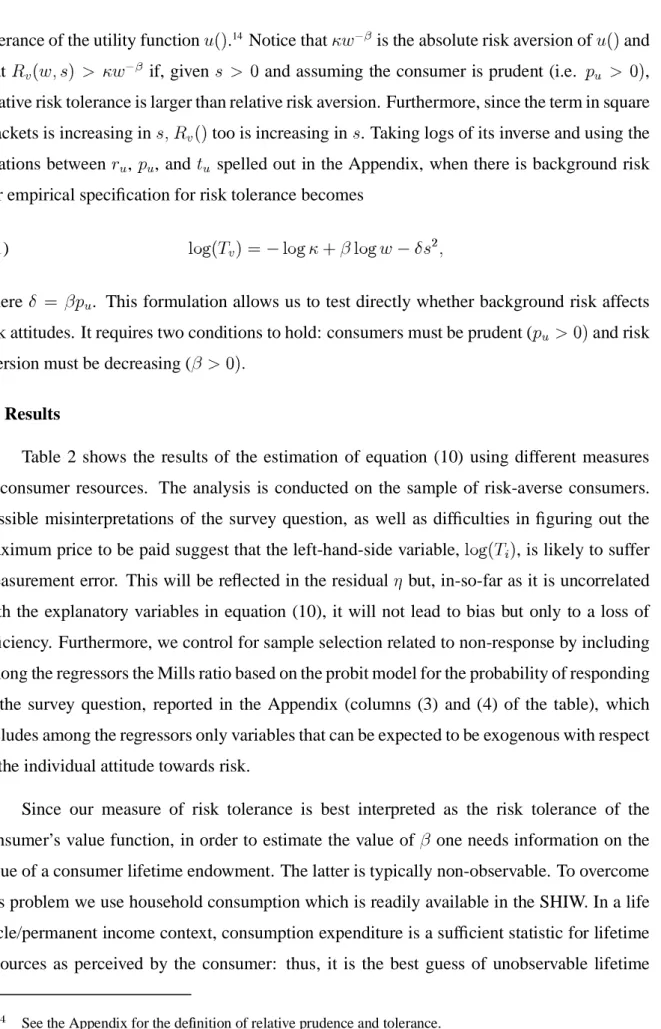
tolerance of the utility functionE.14
Notice thatV3qis the absolute risk aversion ofE and that-Ec r : V3q if, givenr : f and assuming the consumer is prudent (i.e. R : f, relative risk tolerance is larger than relative risk aversion. Furthermore, since the term in square brackets is increasing inrc -E too is increasing in r. Taking logs of its inverse and using the relations between o,R, and | spelled out in the Appendix, when there is background risk our empirical speci¿cation for risk tolerance becomes
*L}EA ' *L} V n q *L} Br2c
(11)
where B ' qR. This formulation allows us to test directly whether background risk affects risk attitudes. It requires two conditions to hold: consumers must be prudent (R : f and risk aversion must be decreasing (q : f
5. Results
Table 2 shows the results of the estimation of equation (10) using different measures of consumer resources. The analysis is conducted on the sample of risk-averse consumers. Possible misinterpretations of the survey question, as well as dif¿culties in ¿guring out the maximum price to be paid suggest that the left-hand-side variable,*L}EA, is likely to suffer measurement error. This will be reÀected in the residual # but, in-so-far as it is uncorrelated with the explanatory variables in equation (10), it will not lead to bias but only to a loss of ef¿ciency. Furthermore, we control for sample selection related to non-response by including among the regressors the Mills ratio based on the probit model for the probability of responding to the survey question, reported in the Appendix (columns (3) and (4) of the table), which includes among the regressors only variables that can be expected to be exogenous with respect to the individual attitude towards risk.
Since our measure of risk tolerance is best interpreted as the risk tolerance of the consumer’s value function, in order to estimate the value of q one needs information on the value of a consumer lifetime endowment. The latter is typically non-observable. To overcome this problem we use household consumption which is readily available in the SHIW. In a life cycle/permanent income context, consumption expenditure is a suf¿cient statistic for lifetime resources as perceived by the consumer: thus, it is the best guess of unobservable lifetime
endowment. However, we also check our results using as proxies for the endowment measures of accumulated¿nancial and total wealth and human wealth, as measured by income.
Assuming that consumption is proportional to the endowment , i.e. S ' b, our empirical speci¿cation becomes
*L}EA ' *L} Vn q *L} S Br2c
(12)
where V ' Vb The ¿rst set of results that we present ignores the potential endogeneity of consumption and wealth as they are themselves affected by preference parameters. In the
¿rst column of Table 2 we report the results from the regression of ,J}EA only on (log)
non-durable expenditure and do not include any consumer characteristics that can proxy for differences in tastes. The estimate ofq is 0.0922 and is highly statistically signi¿cant leading to the rejection of preferences with constant absolute risk aversion. The estimated value ofq implies that absolute risk aversion declines with wealth but at a rate that is far slower than that implied by constant relative risk aversion preferences. In fact, the hypothesis thatq = 1 can be strongly rejected (8 =1,584). It follows that absolute risk tolerance is a concave function of consumer resources.
In the second column of the table we include a set of strictly exogenous individual characteristics, such as age, gender, education attainment (a dummy equal to 1 if the head of the household has completed eighth grade), and dummies for the presence of siblings and for the region of birth. If tastes are impressed in our chromosomes or evolve over life in a systematic way or depend on one’s education15
or are affected by the culture of the place of birth or by the possibility of relying on the support of a brother or sister, then these variables should have predictive power. The analysis shows that only education and the region of birth in fact do, with risk aversion being higher among the least educated. Being male has a negative effect on the degree of risk aversion, but it is not statistically signi¿cant. Furthermore, a test of the hypothesis that the coef¿cients on age, gender, education and siblings are jointly equal to zero cannot be rejected at the standard levels of signi¿cance (8 = D.50, R-value =
48 Education can depend to some extent on the individual attitude towards risk, especially when it comes to
enrollment in higher education. Hence, in the regressions we control only for eighth grade attainment, which can be considered exogenous and determined by factors that are independent of the individual attitude towards risk .
0.2400). Finally, the joint signi¿cance of the 19 regional dummies16
included in the regression, capturing the region of birth, cannot be rejected (see the bottom of Table 2). Furthermore, the coef¿cients on these dummies (not shown) reveal a pattern: compared with those born in the central and southern regions, consumers born in the North are somewhat less risk-averse. One possible interpretation is that the dummies are capturing regional differences in culture, which are transmitted by upbringing. In addition to these variables, we insert in the regression also two dummies for the occupation of the father of the household head: the¿rst dummy is equal to 1 if the consumer’s father is/was self-employed (zero otherwise) the second dummy is equal to 1 if he is/was a public sector employee (zero otherwise). This allows us to test whether parents’attitudes towards risk - as reÀected in their occupation choice - are transmitted to their children. The estimates show that none of these variables has a signi¿cant effect on the degree of risk aversion, although the signs on the dummies turn out as expected and imply relatively lower (higher) risk tolerance among those individuals whose father was a public employee (self-employed), which can be thought of as symptomatic of greater (lower) aversion to risk.
The last two columns of the table report a set of results based on other proxies of the endowment: the¿rst consists of total wealth, which is de¿ned as the sum of real and ¿nancial assets, net of debt, and household income (excluding asset income), which proxies for human wealth the second consists of just the liquid component of household wealth, i.e. ¿nancial assets plus household income (excluding asset income). The basic ¿ndings are con¿rmed: absolute risk tolerance is an increasing and concave function of wealth (total or liquid) and CRRA preferences are strongly rejected. The estimated elasticity of absolute risk aversion to total wealth is lower than to consumption, whereas that to liquid wealth is not signi¿cantly different. In all cases most of the variance of observed risk tolerance is left unexplained, as the low -2r show, suggesting that most of the taste heterogeneity across consumers cannot be accounted for by the set of exogenous variables that we observe. The estimated relation between absolute risk tolerance and consumer resources is consistent with Arrow’s (1965) hypothesis that absolute risk aversion should decrease as the endowment increases while relative risk aversion should increase: but the latter is consistent with the former only if the wealth elasticity of absolute risk aversion is less than one, as our¿ndings indicate.
49 Italy is divided into 20 regions and 95 provinces. The latter correspond broadly to US counties. We will
use the provincial partitioning in Section 7 where we look at the effect of background risk and liquidity constraints on risk aversion.
The Mills ratio, which has been included in all regressions to correct for any selection bias due to systematic non-response, has a small insigni¿cant coef¿cient, which suggests that self-selection is unlikely to be an issue and lack of control should not bias the estimatedq.
The results in the ¿rst two columns of Table 2 have been obtained assuming that consumption is proportional to the endowment, so that the marginal propensity to consume out of wealth is constant. There is a large literature that argues that, in the presence of uncertainty, with prudent behavior, the marginal propensity to consume is large for low values of wealth and tends to the (constant) perfect foresight value as wealth gets large (see Carroll and Kimball, 1996). Thus, consumption will be a concave function of the endowment, implying that the estimated value ofq in equation (12) will reÀect not only the elasticity of the risk aversion of lifetime utility to, but also the elasticity of consumption to . It is easy to show that if this is the case our estimate ofq is larger (in absolute terms) than the true value17, implying that, if
anything, risk aversion declines with the endowment less fast than we estimate. Thus, without knowledge of the consumption function we can only establish an upper bound for the value of
q
6. Robustness
6.1 Endogenous consumption and wealth
The results we have reported so far do not take into account that consumption and wealth are endogenous variables which are themselves affected by consumer preferences. Thus, the estimated coef¿cients are potentially affected by endogeneity bias. The direction of the bias, however, is not clear a priori. If more risk-averse individuals choose safer but less rewarding prospects, they may end up poorer and consume less than the less risk-averse. This would tend to overstate the positive relation between risk tolerance and wealth. However, if the more risk-averse are also more prudent, ceteris paribus, they will compress current consumption, save more and end up accumulating more assets.18 In this case, our estimates of the relationship
4: To see this, letf @ f+z,z which implies z @ f
f+z,. Hence: orj z @ +orj f orj f+z,,. We can
then deal with this like with an omitted variable problem because it is as if we did not include in the regression orj f+z,. The estimated coef¿cient on orj f will be given by h=^4 Fry+orj f> orj f+z,,@Y du+orj f,`. Since the covariance is negative (the larger the level of consuptionf, the smaller the propensity to consume the last unit of wealth), hA.
4; Risk aversion and prudence usually go together. If the utility function is exponential, absolute risk aversion
and prudence are measured by the same parameter if it is CRRA, absolute prudence is equal to absolute risk aversion +4@f if preferences are described by equation (11) absolute prudence is equal to absolute risk aversion
between risk tolerance and wealth will be biased towards zero, which could partly explain why, according to our estimates, risk tolerance increases only slightly as wealth increases.19On the
other hand, the relation between risk tolerance and consumption would be biased downward, implying that the true elasticity of absolute risk aversion to consumption is even less than we obtain.
To address this issue we re-estimate equation (10) with instrumental variables. Finding appropriate instruments for consumption and wealth is no easy task. We rely on the following sets of instruments. First, we use characteristics of the father of the head of the household, namely his education and year of birth, on the ground that wealth is likely to be correlated with that of one’s family, proxied by the father’s education and cohort. Second, we employ measures of windfall gains, such as a dummy for the house being acquired as a result of a bequest or gift, the value of insurance settlements and other transfers that have been received and an estimate of the capital gain on the house since the time of acquisition. Overall, the instruments explain around 30 percent of the variance of (log) non-durable consumption and of (log) total wealth and over 25 percent of the variance of (log) liquid wealth.
Table 3 shows the results when consumption, total wealth and liquid wealth are used. We report the speci¿cation including age, gender, education, siblings, occupation of the father of the head of the household and region of birth. Since for some agents the information on their parents’ characteristics or some other instruments was missing the sample size is by about 300 observations smaller than for the OLS estimates.20 When consumption and liquid wealth
are used as a measure of consumer endowment, the instrumental variable estimates result in a larger estimate of the parameter q. For instance, when consumption is used the estimated
q is 0.1549, more than twice the OLS estimate. But the difference with respect to the OLS
+@f=
4< Another possible explanation of our results is the presence of measurement error in consumption or wealth,
which is a potential source of attenuation bias. To verify whether attenuation is an issue, we have instrumented consumption with total wealth and with total and liquid wealth and have obtained estimates of equal to 0.15 and 0.20, respectively. Instrumenting total wealth with consumption and with consumption and liquid wealth yields estimates of equal to 0.05 and 0.07, respectively. Finally, instrumenting liquid wealth with both consumption and total wealth yields estimates of equal to 0.08. These results suggest that attenuation bias could in fact be an issue, especially when measuring the endowment with total wealth and¿nancial wealth, which are known to be measured with error. However, overall, our conclusions do not change signi¿cantly.
53 Differences in results between the OLS and the IV estimates are not due to differences in the sample.
estimates does not change the previous conclusions: absolute risk aversion is a decreasing function of wealth and both CARA and CRRA preferences are rejected. Figure 2 shows the risk tolerance-consumption relation when the OLS and IV estimators are used: in both cases the pro¿le is far from linear as would be the case under constant relative risk aversion.
To further verify the robustness of our results, we have estimated our basic instrumental variable speci¿cation on a restricted reference sample of 2,200 households. This was obtained from the sample of risk-averse consumers by excluding households with net worth below 20 million lire (623 observations), corresponding to twice the gain from our hypothetical security, and with non-positive income (excluding asset income 13 observations) (in fact, it could be argued that responses are affected by the size of the risky prospect that individuals face) those who reported non-positive¿nancial assets (145 observations), in an attempt to take into account mis-reporting and under-reporting of assets and those who are either too young or too old (below age 21 or above age 75, 57 observations) on the ground that dif¿culties in grasping the lottery question should probably be concentrated at the two tails of the age distribution. The results using consumption as a measure of the endowment, shown in the last column of Table 3, con¿rm those obtained on the whole sample, shown in the ¿rst column, although the estimate is hardly signi¿cant.21
6.2 Quantile regressions
Finally, we check our results for departure of the distribution of residuals from symmetry by estimating least absolute deviation regressions using Amemyia (1982) two-stage estimator to account for endogeneity bias. Given the considerable heterogeneity in the measure of risk aversion, quantile regressions may help give a sense of the determinants of risk aversion for the median consumer. In addition, unlike the conditional mean, quintiles are invariant to monotonic transformations such as taking logs, as we do in equation (10), our empirical speci¿cation. Table 4 shows the results from the estimation when non-durable consumption,
54 Another possibility is that the quality of our indicator of risk aversion depends on the size of the investment
relative to the resources of the consumer in particular, it may be that the investment is too large for some consumers making them unwilling to accept. Notice that the framing of the question is such that the consumer chooses the maximum loss he is willing to incur, which he can choose as small as he wishes. To address this issue further we have estimated our basic equation based on non-durable expenditure splitting the sample below and above median wealth. Results are very similar to those for the whole group. The OLS estimate of is 0.06 for households with below median total wealth and 0.05 for those with above median wealth. Both coef¿cients are statistically signi¿cant but we cannot reject the hypothesis that they are equal.
total wealth and liquid wealth are alternatively used to measure the endowment.22
The main predictions of the OLS and IV analysis reported in Tables 2 and 3 are con¿rmed: for the median consumer absolute risk aversion declines with the endowment and the sensitivity is somewhat larger for consumption and liquid wealth than for total wealth. Furthermore, the estimates ofqc though signi¿cantly different from zero (contrary to CARA preferences) are far below 1 in absolute value (rejecting the CRRA utility).
7. Risk aversion and background risk
In a world of incomplete markets the attitude towards risk, measured by the willingness to accept a fair lottery, may vary between consumers not only because of differences in taste parameters but also because they face different environments. In Section 2 we discuss how risk aversion can be affected by background risk. In this Section we test whether the attitudes towards risk are affected by the presence of uninsurable, independent risks and by the possibility of being liquidity-constrained in the future. To measure background risk we rely on per-capita GDP growth at the provincial level for the period 1952-1992, which we use to compute a measure of the variability of GDP growth in the province of residence. For each province we regress (log) GDP on a time trend and compute the residuals. We then calculate the variance of the residuals and attach this estimate to all households living in the same province. The main advantage of this variable compared with subjective measures of future income uncertainty, such as those analyzed by Guiso, Jappelli and Pistaferri (2002), is that it is likely to be truly exogenous and so, unlike the subjective measures which reÀect occupational choice, less subject to self-selection problems.23
The variance of GDP growth in the province is an estimate of aggregate risk and should be largely exogenous to the individual risk attitude unless risk-averse consumers move to provinces with low variance GDP.
55 Notice that we do not control for sample selection because the Mills ratio accounts for shifts in the mean,
whereas the focus here is on the median.
56 The 1995 SHIW contains a special section in which households are asked a set of questions designed
to elicit the perceived probability of being employed over the twelve months following the interview and the variation in earnings if employed. Guiso, Jappelli and Pistaferri (2002) use these data to obtain an estimate of expected earnings and their variance. They show that the subjective variance is negatively correlated with a dummy for risk aversion and interpret this as evidence of self-selection. When we use the subjective measure of earning uncertainty as a proxy for background risk we¿nd that its effect on risk tolerance is positive, small and not statistically signi¿cant, showing that self-selection nulli¿es any background risk effect, which implies that subjective measures are inadeguate to isolate the effect of background risk on an individual willingness to bear risk.
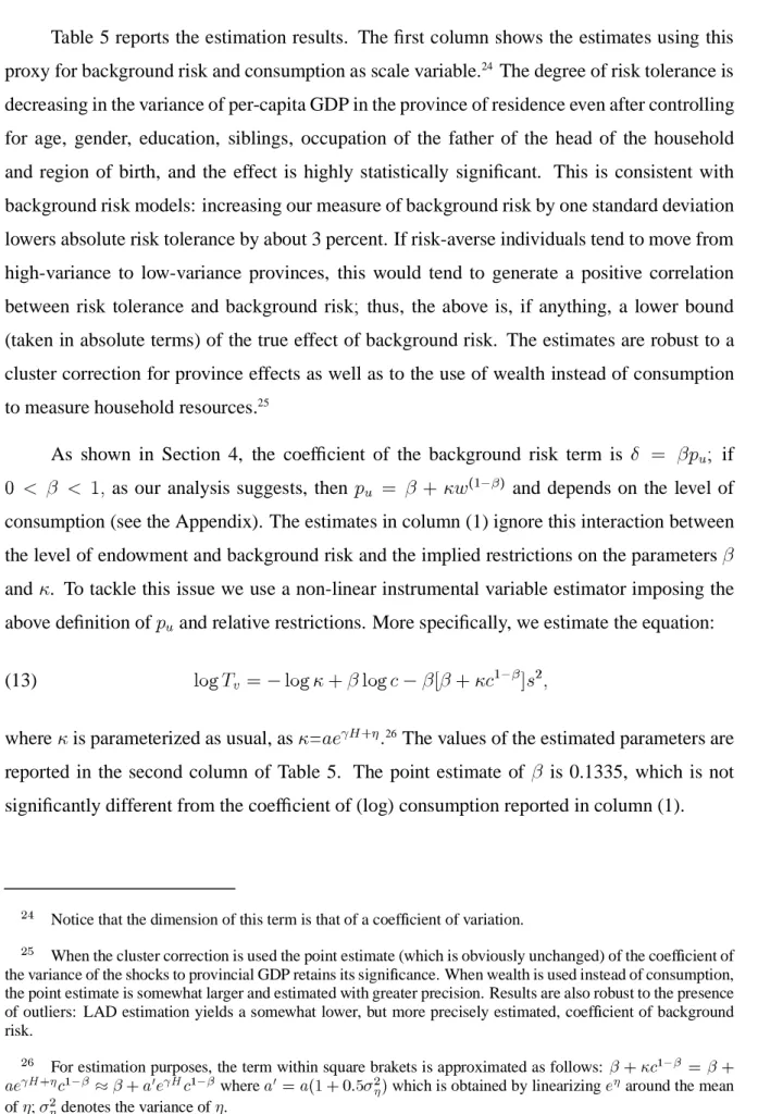
Table 5 reports the estimation results. The¿rst column shows the estimates using this proxy for background risk and consumption as scale variable.24 The degree of risk tolerance is
decreasing in the variance of per-capita GDP in the province of residence even after controlling for age, gender, education, siblings, occupation of the father of the head of the household and region of birth, and the effect is highly statistically signi¿cant. This is consistent with background risk models: increasing our measure of background risk by one standard deviation lowers absolute risk tolerance by about 3 percent. If risk-averse individuals tend to move from high-variance to low-variance provinces, this would tend to generate a positive correlation between risk tolerance and background risk thus, the above is, if anything, a lower bound (taken in absolute terms) of the true effect of background risk. The estimates are robust to a cluster correction for province effects as well as to the use of wealth instead of consumption to measure household resources.25
As shown in Section 4, the coef¿cient of the background risk term is B ' qR if
f q c as our analysis suggests, then R ' q n VE3q and depends on the level of
consumption (see the Appendix). The estimates in column (1) ignore this interaction between the level of endowment and background risk and the implied restrictions on the parametersq and V. To tackle this issue we use a non-linear instrumental variable estimator imposing the above de¿nition of R and relative restrictions. More speci¿cally, we estimate the equation:
*L} A ' *L} V n q *L} S qdq n VS3qor2c
(13)
whereV is parameterized as usual, as V=@eMn#26
The values of the estimated parameters are reported in the second column of Table 5. The point estimate of q is 0.1335, which is not signi¿cantly different from the coef¿cient of (log) consumption reported in column (1).
57 Notice that the dimension of this term is that of a coef¿cient of variation.
58 When the cluster correction is used the point estimate (which is obviously unchanged) of the coef¿cient of
the variance of the shocks to provincial GDP retains its signi¿cance. When wealth is used instead of consumption, the point estimate is somewhat larger and estimated with greater precision. Results are also robust to the presence of outliers: LAD estimation yields a somewhat lower, but more precisely estimated, coef¿cient of background risk.
59 For estimation purposes, the term within square brakets is approximated as follows: . f4 @ .
dhK.f4 . d3hKf4 whered3@ d+4 . 3=85
, which is obtained by linearizing haround the mean
The third column of Table 5 adds to our basic speci¿cation an indicator of liquidity constraints. As argued by Gollier (2000), liquidity constraints act to reduce the consumer horizon, thus limiting the opportunities to time-diversify any risk currently taken, accentuating risk aversion. Our measure of risk aversion is based on the notion that it is liquidity constraints that matter and the danger of their being caused by an inability to borrow and by impediments to draw down accumulated assets in order to increase consumption.27 Thus, the
liquidity-constrained are those who have been refused credit or have not asked believing their request would be turned down (3 percent of the sample), or have a ratio of liabilities to total assets above 25 percent (9 percent of the sample) or have ¿nancial assets representing less than 1 percent of net worth (17 percent of the sample). Overall, we classify as potentially liquidity-constrained around 26 percent of the households in our sample of respondents. The estimated coef¿cient of this indicator has the expected negative sign and is statistically signi¿cant, implying that being liquidity-constrained (or in danger of becoming so) makes agents more risk averse. Economically, being liquidity-constrained lowers risk tolerance by 4.4 percent. This result is robust to the inclusion in the regression of the variance of provincial GDP, as shown in the last column of the table, implying that background risk is not proxying for liquidity constraints.
8. Consistency with observed behavior
If our ¿ndings on the relation between risk tolerance and wealth do indeed reÀect the structure of individual preferences, then this should be reÀected in actual behavior i.e. observed behavior should be consistent with the shape of the measured risk-tolerance-wealth relation. In this section we discuss some implications of our empirical characterization of the wealth-risk-tolerance relation. First, if relative risk tolerance is decreasing in wealth, as implied by our¿ndings, the portfolio share of risky assets should decline as wealth increases. Second, if, as our results suggest, absolute risk tolerance is a concave function of the consumer endowment, the portfolio share of risky assets should be an increasing function of age. Third, if our estimates do indeed identify the parameters of the consumers’ utility function, they should be coherent with those based on the estimation of Euler equations for consumption.
5: If households have low liquid assets, it can be relatively dif¿cult to smooth consumption when confronted
with an unexpected negative income or expenditure shock. If liquid assets are low, to increase consumption households might have to tap into their accumulated assets or ask for credit, which might be costly options. Besides, if they are already heavily in debt, the cost of raising more credit might be very high. Hurst (2000) provides further arguments for using this de¿nition of liquidity-constrained households.
8.1 Wealth-portfolio relation
The¿rst implication is clearly contradicted by the data since portfolio shares are found to be an increasing function of wealth. This is obviously in contrast also with constant relative risk aversion preferences. One strategy that has been pursued in the literature is to maintain the CRRA characterization of the utility of consumption but to assume that wealth enters the utility function directly as a luxury good, for instance through a joy-of-giving/bequest motive. As Carroll (2000) shows, this implies that a larger proportion of lifetime wealth will be devoted to the risky assets. Clearly, this mechanism can still explain the data even if the utility function of consumption is characterized by increasing relative risk aversion (IRRA), provided that the joy-of-giving motive is suf¿ciently strong. Another explanation is that there are portfolio management costs that decline with the size of the investment in risky assets (which is increasing in wealth) if they are suf¿ciently important, this mechanism can overturn any incentive to lower the portfolio share of risky assets coming from IRRA. A third possibility, analyzed by Peress (2001), is that households face costs of acquiring ¿nancial information. Since wealthier consumers tend to invest larger amounts in stocks they have more incentives to invest in information acquisition. Being more informed, in turn, they tend to invest a larger share than the less informed consumers and this mechanism can again counteract the tendency of the portfolio share to decrease due to IRRA. Thus, our results do not, in principle, conÀict with the evidence.
8.2 Age-portfolio pro¿le
To check the second implication - i.e. that with concave risk tolerance the age portfolio pro¿le is upward sloping - we run Tobit regressions of the portfolio share of risky assets on a second-order polynomial in wealth, age and a set of other controls including city size, household size, gender, region of residence, education of the head of the household, etc. We exclude households with zero wealth and those whose head is over 60 since the elderly may have various incentives to decumulate assets after retirement, particularly the riskier ones.28
5; As pointed out by Hurd (2000) the portfolio behaviour of retired elderly consumers may be quite different
from that of the non-retired. First, the retired have a limited ability to return to the labor force and to use this possibility as a buffer against¿nancial losses. This limitation should reduce their willingness to hold risky assets. Second, the elderly face substantial mortality risk, which increases sharply at advanced old age and leads to a decline in consumption and wealth. This, in turn, may be reÀected in the portfolio composition. Third, retired consumers have large annuity incomeÀows and the risks associated with those Àows are quite different from the
After these exclusions our sample includes 4,799 households. Table 6 shows the results of the estimates separately when risky assets are divided by total family wealth and by¿nancial wealth, respectively. The¿rst two columns use the whole sample, the last two columns check the results on the sub-sample of consumers who respond to the lottery question and control also for risk aversion. All the estimates show that the share of risky assets is mildly increasing in age, with the portfolio share increasing by 2 percentage points for a 10-year increase in age, which is consistent with our empirical characterization of absolute risk aversion. With CRRA, the share of risky assets is independent of the investor’s horizon, hence of age.
8.3 Euler equation estimates
To further check the consistency of our results with observed behavior we follow a third route. We estimate the value of the parameterq from an Euler equation for consumption under the assumption that the utility function has the form given by equation (9) in the text and assuming that consumption is proportional to lifetime wealth.29 In this case the risk aversion
of the period utility is proportional to that of lifetime utility.30 Suppose there is no background
risk. Using equation (9) the Euler equation for consumption is
i TEV S3q|n q ' E n o|n i TEV S3q | q n |nc (14)
where is the subjective discount factor and |n is an expectational error, orthogonal to all
variables in the information sets of the agents at time t. Thus, we can use these orthogonality conditions and estimate the parameters of equation (13) using a generalized method of moment estimator. If we are uncovering true preference parameters we should obtain values ofq and
risks of earnings. Finally, the elderly face a much a higher risk of health care consumption than the non-elderly, which discourages holdings of risky assets. Consistent with this, Guiso and Jappelli (2000)¿nd that the portfolio share of risky assets declines with age after retirement.
5< We thank Pierre Andrè Chiappori for suggesting this test.
63 As shown by Tiseno (2002), the risk aversion of lifetime utility,U
X+z,> is related to the risk aversion of
period utilityUx+f+z,, by the identity:
Ux+z, @ Ux+f+z,,fz>
wherefzis the marginal propensity to consume out of lifetime endowment. If the latter is constant inz, the risk aversion of the period utility is the same as the risk aversion of lifetime utility, apart from a rescaling factor.
of the implied degree of risk aversion similar to those estimated in the previous sections.31
To estimate (14) we rely on the panel component of the SHIW and pool together the observations for the years 1989, 1991, 1993 and 1995. The SHIW has a rotating panel component, where half of the sample in a given survey is re-interviewed in the subsequent one. Thus, the maximum number of time periods a household can be present is 4. Since our estimator is consistent only when the number of observations along the time dimension is large these results should be regarded as suggestive. Furthermore, as the Euler equation is known not to hold when credit markets are imperfect, we have excluded those households which are likely to be liquidity-constrained, according to the same de¿nition we have used earlier. Our sample consists of an unbalanced panel of about 4,500 households. As a measure of consumption we use household real expenditure on non-durable goods and services, adjusted for household size.32 As a measure of the interest rate we use the return on bank deposits and checking
accounts, which varies over time and across Italian provinces, and impute to each household in a given year and living in a given province the average rate prevailing in that year and province. To account for demographics, we let the parameterV be a function of the age and gender of the head of the household. Year dummies are also included. As instruments in the agents’ time| information set, we use the interest rate lagged one and two periods, a categorical variable for the size of bank deposits, a dummy for the ownership of saving accounts, the herphindal index of bank concentration in the province, a categorical variable for the size of the town where the household lives and the population of the province where the town is located. Results, not shown for brevity, imply a point estimate of the parameterq of 0.1484, which is very close
64 If there is background risk, using the approximate expression for the indirect utility functiony, we can
write the Euler equation for consumption as: x3+f
w.4, @ +4 . u,x3+fw, ^x333+fw.4, x333+fw,`5@5 . w.4
where it has been assumed that the variance of the background risk is time-invariant. Using (9) and letting |w.4 @ h{s+f
4 w.4
4, this condition can be written as:
|w.4@ +4 . u,|w ^fw.4+f4w.4. fw.4,|w.4 fw +f4w . fw ,|w`5@5 . w.4
which again can be estimated by a generalized method of moment estimator.
65 Household per-adult equivalent expenditure is obtained using the following adult equivalence scale: the
head of the household is weighted 1, the other adults in the household are weighted 0.8 and the children are weighted 0.4.
to the range of estimates we have obtained from the relationship between our measures of absolute risk aversion and the consumer endowment.
Overall, we take the evidence in this Section as suggesting that our estimates of the risk aversion-wealth relation are remarkably consistent with observed behavior. To conclude this discussion, we note that our empirical characterization of the relation between risk aversion and wealth also helps to reconcile some portfolio puzzles that have been noticed in the literature. Simulation models, such as those discussed by Heaton and Lucas (2000), reveal that portfolio shares of risky assets close to those observed in reality, simultaneously require three ingredients: a) background risk must be “large” b) it must be positively correlated with stock market returns c) stock holders must have a high degree of relative risk aversion, 8 in Heaton and Lucas (2000) simulations. The¿rst two conditions are met by the rich segment of the population because they own most of the business wealth which is highly volatile (relative to labor income) and co-moves with the stock market. If preferences are well described by our
¿ndings, then it is very likely that stockholders have a degree of relative risk aversion close
to that implied by the Heaton and Lucas simulations. In our sample, the relative risk aversion of the bottom 10 percent of the wealth distribution is 3.7 on average and its consumption is 23.3 million lire ($ 11,500). The consumption of the top 10 percent, who own 61 percent of total risky assets, is $31,000. Thus for the latter, the predicted degree of relative risk aversion, holding other characteristics constant (i.e. place of birth, exposure to background risk, etc.), would be 8.3 (= 3.7 ((consumption of the rich/consumption of the poor)fH2), close to the value required by the Heaton and Lucas simulations (2000).
9. Conclusions
In this paper we construct a direct measure of absolute risk aversion using the 1995 Bank of Italy Survey of Household Income and Wealth. The measure is based on a simple yet powerful question on the maximum price a consumer is willing to pay to buy a security. Its main advantage is that it does not rely on any assumption as to the form of individual utility. As a consequence, it applies not only to the risk-averse, but also to risk-neutral and risk-prone individuals, providing a point estimate of the degree of risk aversion for each individual in the sample. This estimate has then been used to gather direct evidence on the nature of the relationship between individual risk predisposition, on the one hand, and
individual endowment, demographic characteristics and measures of uninsurable risk exposure and liquidity constraints, on the other.
Our ¿ndings suggest that among risk-averse consumers the degree of absolute risk aversion is decreasing in individual endowment - thus rejecting CARA preferences - but the elasticity to consumption is far below the unitary value predicted by the CRRA utility. Consequently, absolute risk tolerance is a concave function of consumer endowment. How reasonable is this¿nding? One way to answer the question is to run the following experiment. Suppose that a consumer with an annual consumption of 10,000 euros ($10,000, roughly the 17th percentile) is willing (at most) to pay 250 euros to buy the security. Then, using equation (6), the implied value of his absolute risk aversion would be 0.3793. Suppose that relative risk aversion is constant. Then, if our consumer had an annual consumption of 50,000 euros (about the 98th percentile of the distribution) his absolute risk aversion would be 0.0379 (fHbD fc fff*Dfc fffand he would report a price of 3,100 euros to acquire the security. This seems an implausibly high ¿gure, very close to the gain offered on the security in the event of success. Intuitively, the CRRA implies that absolute risk tolerance increases “too fast” with consumption. If, instead, absolute risk tolerance increases with consumption at the speed implied by our estimates, the price that the richer consumer would be willing to pay to buy the security would be 750 euros, a¿gure that we think is much more reasonable.
As argued, our ¿ndings are also consistent with the empirical evidence that young households take on relatively less portfolio risk than more mature households. In fact, according to Gollier and Zeckhauser (1997), the concavity of absolute risk tolerance is a necessary and suf¿cient condition for such behavior to be optimal.
Individual risk aversion also appears to be characterized by a substantial amount of unexplained heterogeneity. Consumer attributes and demographic characteristics are of little help in predicting the degree of risk aversion. The only exceptions are education and the region of birth the latter is likely to capture regional differences in risk predisposition and culture that are transmitted with upbringing within the family.
In a world of incomplete markets, individual attitudes towards risk may vary across households not only because of differences in tastes, but also because of differences in the environment. We address this issue by analyzing the impact that income uncertainty and borrowing constraints have on the degree of risk tolerance. We ¿nd unequivocal evidence
that background risk and borrowing restrictions shape consumers’ attitudes to accepting risk. One important implication is that imperfections in ¿nancial markets may discourage entrepreneurship and investment not only because they limit access to external ¿nance but, more directly, because they discourage individuals from bearing risk.
Table 1
DESCRIPTIVE STATISTICS FOR THE TOTAL SAMPLE, FOR THE SAMPLE OF RESPONDENTS AND VARIOUS SUB-SAMPLES
(The figures for consumption, total wealth and financial wealth are sample medians expressed in million lire. The variable “North” includes the following regions: Piemonte, Valle d’Aosta, Lombardia, Trentino Alto Adige, Veneto, Friuli Venzia Giulia, Liguria and Emilia Romagna; “Center” includes Toscana, Umbria, Marche, Lazio, Abruzzo and Molise and “South” includes all the remaining regions. The low risk-averse are those who are willing to bet at least 1 million lire, which is the median of the bet.)
Variable Sample of respondents Total
sample Risk-averse
Risk-lovers and neutral
Total
High Low Total
Age 49.24 47.39 48.50 49.34 48.54 54.23 Male % 77.98 81.16 79.24 93.75 79.84 74.35 Years of education 8.76 9.98 9.25 10.81 9.31 8.03 Married % 77.88 79.64 78.58 87.50 78.95 72.50 No. of earners 1.84 1.86 1.85 1.81 1.84 1.80 No. of components 3.23 3.15 3.20 3.00 3.19 2.94 No. of siblings 2.55 2.33 2.46 1.90 2.44 2.50 Area of birth: North 34.44 44.07 38.27 53.90 38.91 37.43 Center 23.09 20.18 21.94 19.86 21.85 24.75 South 42.47 35.75 39.80 26.24 39.24 37.82 Self-employed % 15.57 20.14 17.38 29.17 17.87 14.23 Public employee % 28.33 26.37 27.55 27.08 27.53 23.26
Value of Z 0.53 3.78 1.82 11.19 2.21
-Abs. risk aversion 0.189 0.110 0.157 -0.005 0.151 -Consumption 30.28 34.35 32.00 41.20 32.40 28.80 Financial wealth 9.97 18.10 12.76 49.58 13.42 10.39 Total wealth 154.95 198.47 170.50 329.85 173.25 155.85 N. of observations 1,998 1,316 3,314 144 3,458 8,135