Picture Maze Generation by Successive Insertion of Path Segment

1

Picture Maze Generation by Successive

Insertion of Path Segment

Tomio Kurokawa

Aichi Institute of Technology, Department of Information Science 7

1247 Yachigusa, Yagusa-cho, Toyota 470-0392, Japan 8 9 10 11 12 . 13

ABSTRACT

Picture maze is a maze on which some picture appears when it is solved. This paper aims to present a very simple method to construct a picture maze. It is always possible to construct a spanning tree on a connected region of a binary picture. A spanning tree connects all vertices on the region. A 2-by-2 extended picture of a connected picture is the one such that each cell in the picture is transformed to four cells which constitute a square block with the cells. Then by analogy, it is always possible to construct a block spanning tree on the extended picture region, where a block is the square unit of four cells. Construction of the block spanning tree and the generation of the corresponding Hamiltonian path can be done at the same time. The Hamiltonian path is constructed along a data structure of a linked list in a simple manner. It traverses every cell on the 2-by-2 extended picture. The similar procedure but with the smaller block with two vertices, instead of four, can be applied to a non-extended picture, an ordinary one, which produces a near Hamiltonian path, which can then be a maze solution path. The near Hamiltonian path traverses nearly all the vertices on the picture, hence depicting a picture on the maze when it is solved. This paper demonstrates the method and its efficiency.

16

Keywords: Maze, Picture Maze, Spanning Tree, Block Spanning Tree, Path Extension, 17 Hamiltonian Path 18 19

1. INTRODUCTION

Maze generation by computing with square grids has been around for some years. The 22

article [1] showed various algorithms to generate a square grid based maze, usually used, 23

relating with graph theory. Hosokawa [2] presented a number of maze generation algorithms 24

with the relation between path, wall, and coordinates. Xu and Kaplan [3] illustrated complex 25

mazes emphasizing aesthetics for the maze. They also introduced a picture maze [4] called 26

'Maze-a-pix' by illustrating a sample picture maze, which is provided by Conceptis, Ltd. [5]. 27

However, the method of the picture maze generation was not given. The internet site of the 28

company shows various picture mazes and states a history of computer generated picture 29

maze. Okamoto and Uehara [6] demonstrated an automatic generation algorithm for a 30

picture maze by constructing a Hamiltonian path which fills up the picture region. However, 31

the path is generated on the 2-by-2 extended picture array. The maze is so constructed in 32

the research that the player obtains the solution path by filling up all the path cells on the 33

maze and by painting the picture region. Hamada [7] and [8] improved the method [6] by 34

enabling to place the start and goal at different positions. Ikeda and Hashimoto [9] illustrated 35

a picture maze generation method by using simulated annealing. Kurokawa, Mori, and 36

Mizuno [10]-[12] took a different approach and demonstrated a method to generate a picture 37

maze by making use of the picture contours. In this method, all the contours are extracted 38

and are incorporated into the picture maze. It is a very flexible method and can be applicable 39

to a wide range of binary pictures. F.J. Wong and S. Takahashi [13] constructed a hybrid 40

picture maze from two photograph images. This maze is not based on square grids like the 41

mazes but on the special grids computed from the image. Two photo pictures are 42

overlapped in the maze. The maze player depicts an outline of one picture on the other 43 picture background. 44

2. MAZE STRUCTURE

There are a number of different representation structures of a square grid maze. This paper 47

uses one of them and it is explained in this section. A computer constructed maze is usually 48

represented by a two-dimensional array. Such a maze consists of path and wall. A path cell 49

is either a vertex or an edge (of a graph). Fig. 1 is a sample maze array of size 7x7---where ' 50

◎' is a vertex; 'e' is an edge, and 'W' and 'w' are walls. A vertex is placed one in every two 51

cells horizontally and vertically. An edge represents the connection between the two vertices. 52

Diagonally adjacent cells to a vertex are wall cells; there are four such cells around a vertex; 53

the vertically or horizontally adjacent cells to a vertex are edge or wall cells. If the cell 54

represents the connection between the two vertices, then it is an edge cell; otherwise it is a 55

wall cell. 56

57

The connection between the two vertices is 4-way, vertical or horizontal; and no diagonal 58

connection is allowed. The entire path routes in a maze organize a spanning tree. A vertex 59

and an edge alternately appear along a path. The maze solution of Fig. 1 is the path from 60

the start (S) to the goal (G), which is one of the paths from a vertex (the tree root) to another 61

vertex (a leaf). The maze structure is kept maintained even if the maze is shifted in any 62

direction one or more positions on the array. However, in Fig. 1, vertices are placed on (odd, 63

odd) coordinates. 64

65

If the walls are thinned [14], the maze becomes as presented in Fig. 2. This maze, to be 66

presented to a player, actually consists of two kinds of cells: path and wall. However, it 67

represents the corresponding graph with vertices and edges, which cannot be otherwise 68

represented as simply as this structure. So the maze of this structure is said to be an 69

elaborately organized graph. The edges play very important roles in this elaboration. Without 70

the edge cells, additional information is required to show how vertices are connected [15]. In 71

short, a maze is said to be a collection of vertices and edges like a graph. However, more 72

restrictions are imposed on a maze: physical positions of vertices and edges; the number of 73

edges to be connected to a vertex and the like. 74 75 76 77 78 79 80 81 82 83

Fig. 1 Maze structure Fig. 2 Maze to be presented to a player 84 1 2 3 4 5 6 7 1 S e ◎ w ◎ e ◎ 2 w W e W e W w 3 ◎ e ◎ e ◎ e ◎ 4 w W e W w W w 5 ◎ e ◎ e ◎ e ◎ 6 e W e W e W e 7 ◎ w ◎ w ◎ w G

3. RELATED PRECEEDING STUDIES

86

Okamoto and Uehara [6] presented a method to generate a picture maze by constructing a 87

Hamiltonian path on the 2-by-2 extended picture. The 2-by-2 extended picture array is 88

constructed by dividing each cell of the original picture array by two, both vertically and 89

horizontally. So each cell of the original picture becomes a square unit of four cells in the 2-90

by-2 extended picture. The Hamiltonian path visits all the vertices on the foreground picture 91

region. So, when the maze player traces the path by filling up all the vertices on the picture 92

region, the hidden picture appears. The reason to use the 2-by-2 extended picture is to 93

guarantee the existence of the Hamiltonian path on the region. The studies of [6] by 94

Okamoto and Uehara and [8] by Hamada explain the algorithm of the maze construction. 95

The algorithm outlines as: 96

97

(1) Prepare a binary picture on square grids; 98

(2) Construct a spanning tree on the picture region; 99

(3) As traveling around the spanning tree by using the right (left) hand rule, construct the 100

Hamiltonian path on the 2-by-2 extended picture; 101

(4) The obtained Hamiltonian path is the solution path of the maze. 102

4. PROPOSED SIMPLE METHOD

104

All experiments in this paper were done by using the free software [16] and [17]. 105

4.1 Constructing a Spanning Tree

As known, it is always possible to draw a spanning tree on a connected region which is on 107

an array of square grid cells. That is, with repeated random extension of a vertex from one 108

starting vertex, an adjacent vertex can be repeatedly connected to the already connected 109

part until no unconnected vertex exists in the region. A spanning tree completes at the end. 110

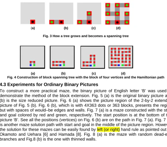
Fig. 3 (a) to (d) illustrates how the tree grows and becomes a spanning tree. In Fig. 3, the 111

larger square is the picture region, where the tree can grow. The red cell with a green dot is 112

the vertex and the darker gray cell is an edge. Staring with the red cell with a black dot, the 113

tree grows as the random connection of an adjacent vertex to the tree proceeds. The 114

connection is made with the edge (dark gray cell). Fig. 3 (d) is the final spanning tree. 115

4.2 Construction of Block Spanning Tree and the Hamiltonian Path

This subsection describes how to construct a Hamiltonian path which fills up all the vertices 117

on the 2-by-2 extended picture simultaneously building the block spanning tree. It is by the 118

analogy of the method of the spanning tree construction in the previous subsection 4.1. 119

120

Each cell in the original picture corresponds to the block of four cells in the 2-by-2 extended 121

picture. This provides the principle that if a vertex extension on the original picture to 122

construct a tree is possible, then the corresponding extension of the block of four vertices on 123

the extended picture is possible. If the extension is repeated until all blocks are connected, a 124

spanning tree with blocks is to be completed on the picture region at the end. This means 125

that it is always possible to construct such a spanning tree on the extended picture. The 126

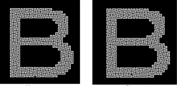
block trees so generated are shown in Fig. 4 (a)-(d), where they are with the simultaneously 127

being generated path which traverses all the vertices of the block trees without repetition of 128

any vertices or edges. Fig. 4 (d) illustrates the block spanning tree as well as the final 129

Hamiltonian path on the picture region. 130

131

Fig. 4 (a) shows the starting block. The extension could be made to three directions: to the 132

right, to the top or to the left. The extension to the bottom is not allowed because it is out of 133

the picture region. Fig. 4 (b) illustrates the second extension made to the left as a random 134

process. The path starts at the vertex with green color, going through the alternating 135

sequence of edge (gray) and vertex (red) and ends at the vertex of blue color. Fig. 4 (b) and 136

(c) are the intermediate results. Fig. 4 (d) is the final block spanning tree and the constructed 137

Hamiltonian path. 138

139

Whenever one square unit of four vertices is added to the tree, four vertices and five edges 140

are connected in the proper order and one edge at the extending position is deleted so as to 141

make the path go through all the vertices which constitute the tree being constructed. When 142

the tree finally becomes a block spanning tree, the path becomes the Hamiltonian path for 143

the final block tree, which fills up all the vertices on the extended picture region. If the final 144

block tree is a block spanning tree, the final path is the Hamiltonian path. 145

146

To construct the Hamiltonian path and the block spanning tree at once, a data structure of 147

linked list is useful and efficient to hold the positions of vertices and edges for the path being 148

organized. The list, which is the linked nodes of x, y coordinates of cell position and vertex 149

number, holds the sequence of vertices and edges in the order for which the vertices and 150

edges appear on the path. Use of the list provides an efficient way to find the path place 151

where the next block path segment is to be connected as well as to insert a path segment 152

into the path. It makes it needless to traverse the tree while constructing the Hamiltonian 153

path. By this method, the block spanning tree and the Hamiltonian path are constructed at 154

once. An experimentally organized list is illustrated in section 6. 155 156 157 158 159 160 161 (a) (b) (c) (d) 162 163

Fig. 3 How a tree grows and becomes a spanning tree 164 165 166 167 168 169 170 171 (a) (b) (c) (d) 172

Fig. 4 Construction of block spanning tree with the block of four vertices and the Hamiltonian path 173

4.3 Experiments for Ordinary Binary Pictures

To construct a more practical maze, the binary picture of English letter ‘B’ was used to 175

demonstrate the method of the block extension. Fig. 5 (a) is the original binary picture and 176

(b) is the size reduced picture. Fig. 6 (a) shows the picture region of the 2-by-2 extended 177

picture of Fig. 5 (b). Fig. 6 (b), which is with 4X363 dots or 363 blocks, presents the region 178

but with spaces of would–be edges and walls. Fig. 7 (a) is a maze constructed with the start 179

and goal colored by red and green, respectively. The start position is at the bottom of the 180

picture ‘B’. See all the positions (vertices) on Fig. 6 (b) are on the path in Fig. 7 (a). Fig. 7 (b) 181

is another maze solution path with start and goal in the middle of the picture region. However, 182

the solution for these mazes can be easily found by left (or right) hand rule as pointed out by 183

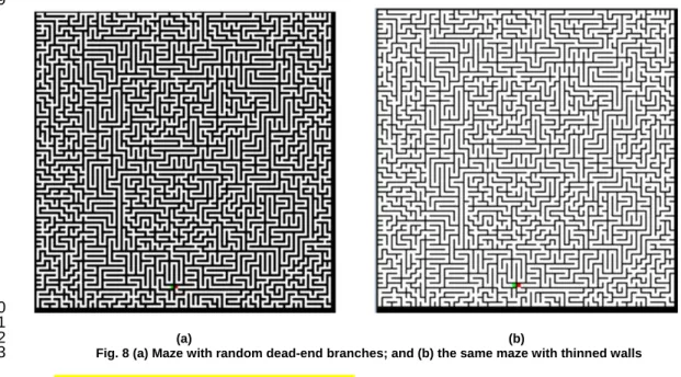
Okamoto and Uehara [6] and Hamada [8]. Fig. 8 (a) is the maze with random dead-end 184

branches and Fig.8 (b) is the one with thinned walls. 185

186 187

188 189 190 191 192 193 194 195 (a) (b) 196 197

Fig. 5 Original binary picture (a); and (b) the reduced one by 4 198 199 200 201 202 203 204 205 206 207 208 209 (a) (b) 210 211

Fig. 6 (a) 2-by-2 extended picture; and (b) the one with would-be edges inserted 212

213

214

(a) (b) 215

Fig. 7 (a) Block Hamiltonian path with the start and goal at the bottom; and (b) block Hamiltonian path with 216

the start and goal in the middle of the picture. 217

219

220 221

(a) (b) 222

Fig. 8 (a) Maze with random dead-end branches; and (b) the same maze with thinned walls 223

5. A METHOD WITH SMALLER BLOCK

5.1 Constructing a Near Hamiltonian Path

Another block extension method was tried to demonstrate the picture maze generation using 226

an ordinary binary picture instead of the 2-by-2 extended one. In this case, the smaller block, 227

which includes only two vertices instead of four, was used to extend the path. As Fig. 9 (a) 228

illustrates, it starts with the two vertices (green and blue) and the edge between the two. The 229

first extension is upward as shown by Fig. 9 (b). Two vertices and three edges are also 230

inserted into the list in the proper order as done in the block method with four vertices of the 231

previous section. The spanning tree completes as in Fig. 9 (d). This method is supposed to 232

be more flexible because the block is smaller. Similar operations appear in the studies [9] by 233

Ikeda and Hashimoto and [13] by Wong and Takahashi, but in different situations. 234 235 236 237 238 239 240 (a) (b) (c) (d) 241

Fig. 9 Construction of block spanning tree with the block of two vertices and the Hamiltonian path 242

243

5.2 Practical Application

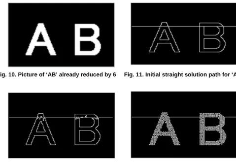
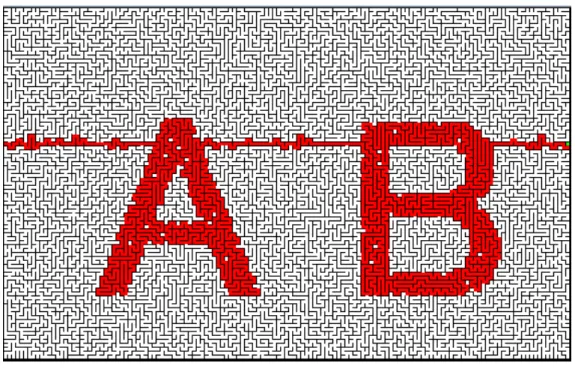
A practical but simple picture of letters ‘AB’ was tried for a demonstration. Fig. 10 is the 245

picture of ‘AB’ which was reduced by 6 from an original picture. The maze was to be 246

constructed from this reduced picture by employing the method of subsection 5.1. In this 247

case, the picture was not extended. Fig. 11 illustrates the initial path which is just a straight 248

path, the simplest, from the entrance vertex (a green point at the extreme right) to a 249

boundary position of the exit vertex (a red point at the extreme left) passing through both of 250

the foreground picture parts of ‘AB’. There are two regions in which the path grows---‘A’ and 251

‘B’. Those are the foreground parts of ‘AB’. The contours of ‘AB’ in Fig. 11 are just to show 252

where the initial path line goes through. The contours are not directly related with the path 253

construction. Fig. 12 shows an early stage of the path extension. The extension occurs in 254

both regions of ‘A’ and ‘B’; where a Hamiltonian path is tried to be generated. This means 255

that the entire path from the entrance to the exit was constructed at once. More importantly, 256

those initial extensions are made in both directions upward and downward in many positions. 257

Therefore the maze cannot be solved easily with only one of the left or right hand rules. The 258

path is constructed with the mixed rules. The details are given in section 6. 259

260

Fig. 13 is a completed maze solution path. A number of black dots are seen. These are the 261

vertices not on the maze solution path. The path failed to become a Hamiltonian path.

262

Therefore, it should be called as a near Hamiltonian path. The complete avoidance of the black

263

points is usually impossible. This is probably why the 2-by-2 extended picture was used in the

264

study [6]. However, the picture ‘AB’ appears clearly in Fig.13.

265 266

Since the straight path lines are often easily seen before the solution is obtained [12], some 267

zigzags were added to hide them, using the same path extension method, as shown in Fig. 268

14. By the way horizontal and vertical straight lines or slopes with near 45 degree are often 269

easily seen before the maze is solved. After dead end branches were added and walls were 270

thinned, the final maze was finished as in Fig. 15. Fig. 16 is the maze with the solution path. 271

272

By the way, some more general procedures were suggested in the studies [9] and [13] for 273

the initial path generation. 274 275 276 277 278 279 280 281 282 283 284 285

Fig. 10. Picture of ‘AB’ already reduced by 6 Fig. 11. Initial straight solution path for ‘AB’ 286 287 288 289 290 291 292 293 294 295 296 297 298 299 300

Fig. 12. Early stage of solution path construction for ‘AB’ Fig. 13. Final solution path for ‘AB’ 301

302 303

Fig. 14. Final solution path with zigzag for ‘AB’ 304

305 306

307

Fig. 15. Final maze for ‘AB’

309

310

Fig. 16. Picture maze of ‘AB’ solved 311

6. DISCUSSION

In this subsection, more details are given about the construction of the block spanning tree 313

and the corresponding Hamiltonian path. 314

6.1 Outline of the Algorithm for the Hamiltonian Path Construction

Fig. 17 to 19 illustrate how the tree and the path are developed on the same picture region 316

as Fig. 4, that is, the 2-by-2 extended picture region with 9 blocks. The path construction 317

algorithm is given as: 318

319

1) Construct the path of the initial block in the array and the list (Fig. 17 (a) and (b) );

320

2) Find a proper position on the path to which a new block is connected;

321

3) Delete one edge between the two vertices (at the above proper position) to which next block path

322

segment is inserted. Put the four vertices and the five edges in the appropriate order on the array

323

and insert them into the list at the position so that the vertices and edges together organize one

324

path;

325

4) Repeat 2) to 3) until all blocks are connected.

326 327

Fig.17 to Fig.19 illustrates only the model case. However, the above algorithm is applicable 328

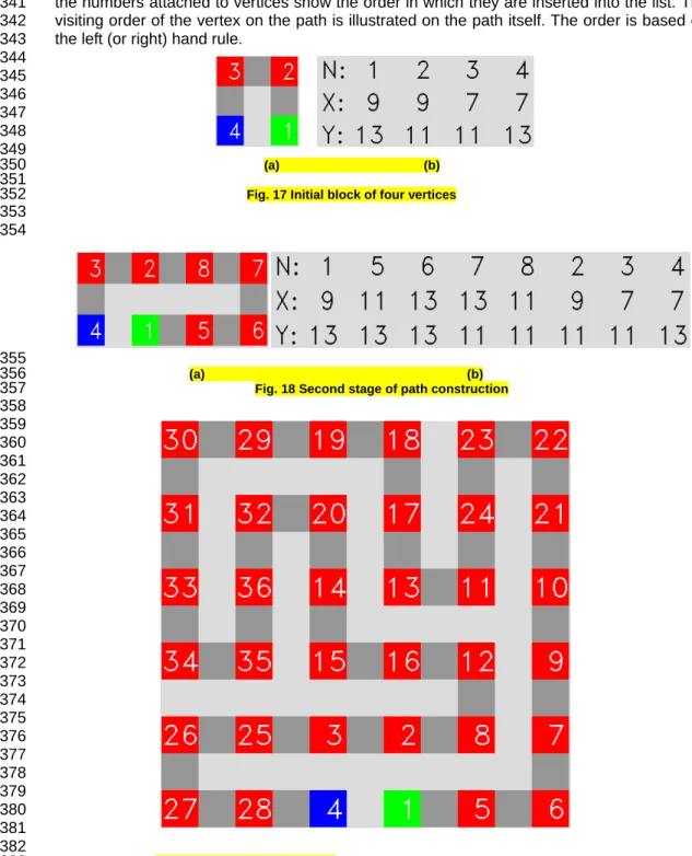
to more practical pictures, which will be later explained. Fig. 17 (a) is the initial path with the 329

numbered vertices. The number, though not required for the path construction, explains the 330

order in which the vertices are inserted into the list. Fig. 17 (b) shows the list on which the 331

number and x and y coordinate addresses on the maze array and along the path are written. 332

This illustrates that the path starts with the vertex of ‘1’ and visiting the vertices in the order 333

‘2’, ‘3’, and ‘4’ which is the goal. x and y addresses of vertices ‘1’ to ‘4’ agree between Fig. 334

17 (a) and (b). Fig. 18 (a) and (b) show the situation where the second block is connected. 335

The vertex sequence in the list is in Fig. 18 (b) which also well corresponds with Fig. 18 (a). 336

What was actually done is as follows: Given the situation of Fig. 17, the edge between 337

vertices ‘1’ and ‘2’ was first removed and then an edge and a vertex were inserted 338

alternately with the vertex order of ‘5’, ‘6’, ‘7’ and ‘8’. The selection of the list position where 339

to insert the block path segment is the random process. Fig. 19 is the final Hamiltonian path; 340

the numbers attached to vertices show the order in which they are inserted into the list. The 341

visiting order of the vertex on the path is illustrated on the path itself. The order is based on 342

the left (or right) hand rule. 343 344 345 346 347 348 349 (a) (b) 350 351

Fig. 17 Initial block of four vertices 352 353 354 355 (a) (b) 356

Fig. 18 Second stage of path construction 357 358 359 360 361 362 363 364 365 366 367 368 369 370 371 372 373 374 375 376 377 378 379 380 381 382

Fig. 19 Final Hamiltonian path: vertex 30 is at (3,3) and vertex 6 is at (13,13) 383

384 385

6.2 C Program Code, Explanation, Algorithm, Theorem and Proof

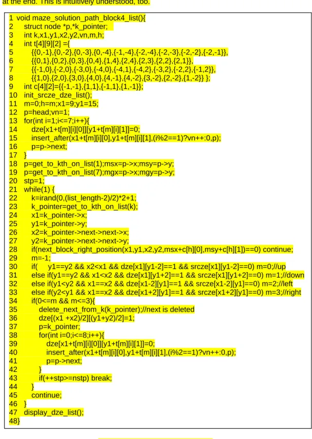
The essential part of the C program code, which actually produced Fig. 17 to Fig. 19 and 387

Fig.7 (with a little change), is given in Fig. 20. This code follows the algorithm given in 388

subsection 6.1. 389

390

C program code explanation:

391

The line 2 defines the pointers. p and k_pointer are the pointers which point to the nodes in 392

the linked list. The node has the fields of the maze array coordinates of x, y, the vertex 393

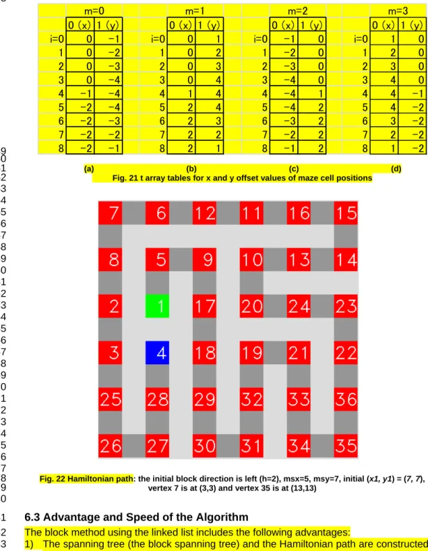
number n and the link next. The array t defined on lines 4 to 8 is to provide offsets for 394

determining x and y position of edges and vertices which are to be inserted into the path. 395

This table array consists of four parts as in Fig. 21, which will be explained later. The path 396

eventually grows to a Hamiltonian path. Line 9 defines table c for the offset values to 397

compute the center position of the initial block from which a Hamiltonian path grows. This 398

table is used on line 28. The function on line 10 does two jobs: first is to make srcze array, 399

the dotted picture like Fig. 6 (b), with 0 for the foreground picture cells and 1 for the 400

background; second is to initialize dze array with all 1, on which the Hamiltonian path is to be 401

constructed with 0 on the path cells. Line 11 gives the start x1 and y1 position and the block 402

extension direction m=0 (up) and h=m (initial block direction). To make the correspondence 403

with the Fig.17 to Fig 19, m=0 (h=0), x1=9, and y1=15 were specified. For these values, the 404

center of the block is (8, 12), and the start vertex (vn=1) is at (9, 13). 405

406

Other m, x1 and y1 can be specified. If m=2 (h=2), x1=7, and y1=7, the Hamiltonian path 407

eventually became as in Fig. 22. By the way, for this model case of 9 blocks, the maze 408

picture array srcze is 0 at all odd positions (odd, odd) within the square from (3, 3) to (13,13), 409

and 1 at other positions. 410

411

Line 12 set p to head (head pointer of the list) and the first vertex number vn to 1. Lines 13 412

to 17 draw the first block path on dze and insert the path into the list. The function 413

insert_after has the following C prototype: 414

415

_ , , , ∗ , (1) 416

417

where x and y are coordinate addresses and vn is the number for the vertex; vn is 0 for all 418

edges. This function inserts the node with the data specified by the parameter into the list. 419

The new node is placed after the node pointed by p. The table t is used for the computation 420

of edge and vertex positions. It has four tables as shown in Fig. 21 (a) to (d). For the initial 421

block path construction, only the table with m=0 is used. m can be one of the four numbers 0, 422

1, 2, and 3. The block direction upward (m=0) is given initially for the given case. With x1 423

and y1 as the base position adjacent to which the initial path segment is constructed, each of 424

x and y positions of the subsequent path cells of edge and vertex to be inserted is given by 425

the following expressions: 426 427 1 0 (2) 428 429 1 1 (3) 430 431

The list and the maze array dze hold the same address data. For the initial path segment, 432

the two edges for i=0 and 8 are not necessary. So they are not inserted. Line 16 is 433

forwarding the list pointer. Lines 18 and 19 are to get the positions of the start and goal 434

vertices which were actually inserted into the list. (msx, msy) is the start and (mgx, mgy) is 435

the goal. Line 20, stp=1, means the initial block path is completed. 436

Line 21 is the start of endless loop, which would finish when all the block path segments are 438

connected. Line 22 generates an odd integer random number k which is from 1 to the length 439

of the list minus 2. On line 23, k_pointer is set to point to the k-th node. On lines 24 to 27, the 440

two positions p1=(x1, y1) and p2=(x2, y2) are obtained as the path positions between which 441

new block path segment is to be inserted. Line 28 is to examine if the above two positions 442

are at proper positions. All the possible block positions are predetermined by the initial block 443

positions. That is, the x and y positions of the center of a block must be as 444 445 ∗ 4, (4) 446 447 ∗ 4, (5) 448 449

If the positions are not proper, a new position is tried on the list as a random process. For 450

this examination, table c is used. It has the offset values from the position (msx, msy) to the 451

block center. Line 29 is just to cancel the direction of the previous insertion. Lines 30 to 33 452

are to set m according to the two positions p1 and p2. p1 is nearer to the list head than p2. 453

Therefore those two positions suggest in which direction the block extension is possible. 454

Based on the implied direction, the feasible extension is examined. If the extension is found 455

possible, m is set to the direction: 0 (the direction is upward), 1 (down ward), 2 (leftward), 456

and 3 (rightward). 457

458

Line 34 is to check if the extension direction has been determined. If so, m must be from 0 to 459

3. If extension is not possible, then another p1 and p2 positions must be tried. Based on the 460

value of m, the path is to be extended. m specifies which table of Fig. 21 (a) to (d) should be 461

used. The tables supply the offset values of x and y positions of the edges and vertices 462

which are to be inserted into the path. Line 35 deletes the node which follows the node 463

pointed by k_pointer. Line 36 removes the edge between p1 and p2 from the path. The both 464

lines are removing the edge from the path. Line 37 sets p to k_pointer to do the next 465

consecutive block path insertion. Lines 38 to 42 repeatedly draw the next block paths on dze 466

and insert them into the list. How to do it is similar to the initial block path construction on 467

lines 13 to 17. For this case, additional edge insertions are included at the first and at the 468

end. Table t is used for the computation of edge and vertex positions as before. But all four 469

tables in Fig. 21 (a) to (d) are possibly used based on m. The computation of x and y 470

positions is according to (2) and (3). vn on line 40 is the vertex number, incremented every 471

time a vertex is inserted as before. stp on line 43 counts the inserted blocks including the 472

start block. nstp holds the number of blocks in the region. If the control reaches line 45, it 473

means path insertion has not been done for the positions p1 and p2. When it reaches the 474

number of the blocks in the foreground picture region, the while loop breaks. The results are 475 displayed on line 47. 476 477 Theorem: 478

The algorithm (C program code) constructs a maze solution path (a Hamiltonian path) on the 479

maze array dze as well as on the list pointed by head under the supposition of the following: 480

1 The maze picture array

srcze

picture. It has

n

2 The maze array

dze

srcze

be constructed on this array

dze

3 A linked list, which is to hold the path, is initialized to be pointed by

head

Proof:

486

When n 1: At the top of the algorithm initialization part , the code construct the first block 487

path. It constitutes the path with the vertices and the edges as 488

489

, (6) 490

where is a vertex and is an edge and is the start vertex and is the goal vertex. 491

The above path is clearly a Hamiltonian path on the region of one block. This means the 492

algorithm constructs a Hamiltonian for n=1. This initial block path construction is given by the 493

program code lines 11 to 17. A proper position for the block is set in the code. 494

495

Suppose the algorithm constructs a Hamiltonian path for n=r, where r is an integer greater 496 than 0: 497 ⋯ ⋯ (7) 498 499

, where and are the vertices between which a new block path is to be inserted and all 500

the block path segments on (7) are on the right positions as specified by (4) and (5). The 501

problem at this point is if and are on the right position or not. This is, however, 502

guaranteed by the function on line 28: 503

504

_ _ _ 1, 1, 2, 2, 0 , 1 . (8)

505 506

This function returns 1, if the position is right; otherwise 0. So if it returns 0, the new position 507

is tried. The decision is based on (4) and (5). 0 1 give the 508

center position of the initial block. There is another problem at this point. It is whether the 509

new block path segment to be connected is within the foreground picture region and the new 510

block path region is an unused one on dze. This problem is resolved by lines 30 to 33. In 511

addition, it provides the direction with m, a right direction to extend to. So a new block is 512

always on a right position and within the foreground picture part. 513

514

Consider that the next block to be connected consists of four vertices and five edges which 515

are counterclockwise sequenced from which is adjacent to as: 516

517

. (9)

518 519

Also consider as the edge to be discarded. 520

521

Since the C program code does the following two: 522

1) Lines 35 and 36 remove the edge from the path of (7); 523

2) Lines 37 to 42 insert (9) into (7) after , 524 (7) becomes as: 525 526 ⋯ ⋯ . (10) 527 528

Since (7) is a Hamiltonian path in r blocks, of (7) is removed and a Hamiltonian path part 529

within the block (9) is inserted into (7), the resultant path becomes a Hamiltonian path in 530

n=r+1 blocks, where all blocks are on the right positions. (10) is the resultant path, which 531

goes through all the vertices on r+1 blocks. See (10) is alternately sequenced by a vertex 532

and an edge and it starts at a vertex and ends at a vertex. 533

534

The remaining problem is if the algorithm can guarantee that all the block paths of n blocks 535

on the foreground part of srcze are to be connected. This problem is resolved automatically. 536

Since the foreground part of srcze is connected, there is always available at least one block 537

to be connected which is adjacent to the already constructed part of the path as long as an 538

unconnected block exists. This completes the proof. 539

540

Since the first block path has four vertices and whenever a new block path (all edges and 541

vertices are alternately sequenced as a path) is connected, four vertices, counterclockwise, 542

are inserted into the path and no vertex is removed. So the Hamiltonian path is constructed 543

at the end. This is intuitively understood, too. 544

545

Fig. 20 Essential part of C program code 546

1 void maze_solution_path_block4_list(){ 2 struct node *p,*k_pointer;

3 int k,x1,y1,x2,y2,vn,m,h; 4 int t[4][9][2] ={ 5 {{0,-1},{0,-2},{0,-3},{0,-4},{-1,-4},{-2,-4},{-2,-3},{-2,-2},{-2,-1}}, 6 {{0,1},{0,2},{0,3},{0,4},{1,4},{2,4},{2,3},{2,2},{2,1}}, 7 {{-1,0},{-2,0},{-3,0},{-4,0},{-4,1},{-4,2},{-3,2},{-2,2},{-1,2}}, 8 {{1,0},{2,0},{3,0},{4,0},{4,-1},{4,-2},{3,-2},{2,-2},{1,-2}} }; 9 int c[4][2]={{-1,-1},{1,1},{-1,1},{1,-1}}; 10 init_srcze_dze_list(); 11 m=0;h=m;x1=9;y1=15; 12 p=head;vn=1; 13 for(int i=1;i<=7;i++){ 14 dze[x1+t[m][i][0]][y1+t[m][i][1]]=0; 15 insert_after(x1+t[m][i][0],y1+t[m][i][1],(i%2==1)?vn++:0,p); 16 p=p->next; 17 } 18 p=get_to_kth_on_list(1);msx=p->x;msy=p->y; 19 p=get_to_kth_on_list(7);mgx=p->x;mgy=p->y; 20 stp=1; 21 while(1) { 22 k=irand(0,(list_length-2)/2)*2+1; 23 k_pointer=get_to_kth_on_list(k); 24 x1=k_pointer->x; 25 y1=k_pointer->y; 26 x2=k_pointer->next->next->x; 27 y2=k_pointer->next->next->y; 28 if(next_block_right_position(x1,y1,x2,y2,msx+c[h][0],msy+c[h][1])==0) continue; 29 m=-1;

30 if( y1==y2 && x2<x1 && dze[x1][y1-2]==1 && srcze[x1][y1-2]==0) m=0;//up 31 else if(y1==y2 && x1<x2 && dze[x1][y1+2]==1 && srcze[x1][y1+2]==0) m=1;//down 32 else if(y1<y2 && x1==x2 && dze[x1-2][y1]==1 && srcze[x1-2][y1]==0) m=2;//left 33 else if(y2<y1 && x1==x2 && dze[x1+2][y1]==1 && srcze[x1+2][y1]==0) m=3;//right 34 if(0<=m && m<=3){ 35 delete_next_from_k(k_pointer);//next is deleted 36 dze[(x1 +x2)/2][(y1+y2)/2]=1; 37 p=k_pointer; 38 for(int i=0;i<=8;i++){ 39 dze[x1+t[m][i][0]][y1+t[m][i][1]]=0; 40 insert_after(x1+t[m][i][0],y1+t[m][i][1],(i%2==1)?vn++:0,p); 41 p=p->next; 42 } 43 if(++stp>=nstp) break; 44 } 45 continue; 46 } 47 display_dze_list(); 48}

547 548 549 550 (a) (b) (c) (d) 551

Fig. 21 t array tables for x and y offset values of maze cell positions 552 553 554 555 556 557 558 559 560 561 562 563 564 565 566 567 568 569 570 571 572 573 574 575 576 577

Fig. 22 Hamiltonian path: the initial block direction is left (h=2), msx=5, msy=7, initial (x1, y1) = (7, 7), 578

vertex 7 is at (3,3) and vertex 35 is at (13,13) 579

580

6.3 Advantage and Speed of the Algorithm

The block method using the linked list includes the following advantages: 582

1) The spanning tree (the block spanning tree) and the Hamiltonian path are constructed at 583

once avoiding pre-generation of an ordinary spanning tree and traveling around it which 584

is described in section 3 and the article [3]. 585

2) The linked list used provides an efficient processing. This may be as a matter of course. 586

3) Only the vicinity of the growing tree is enough to be searched when finding a next block 587

path to be inserted. This may be as a matter of course, too. 588

0 (x) 1 (y)

0 (x) 1 (y)

0 (x) 1 (y)

0 (x) 1 (y)

i=0

0

-1

i=0

0

1

i=0

-1

0

i=0

1

0

1

0

-2

1

0

2

1

-2

0

1

2

0

2

0

-3

2

0

3

2

-3

0

2

3

0

3

0

-4

3

0

4

3

-4

0

3

4

0

4

-1

-4

4

1

4

4

-4

1

4

4

-1

5

-2

-4

5

2

4

5

-4

2

5

4

-2

6

-2

-3

6

2

3

6

-3

2

6

3

-2

7

-2

-2

7

2

2

7

-2

2

7

2

-2

8

-2

-1

8

2

1

8

-1

2

8

1

-2

m=0

m=1

m=2

m=3

589

By the way, the program execution on the personal computer (MAC PRO with 2x2 2.8 GHz 590

Quad-Core Intel Xeon; purchased Feb. 2008) finished in a moment for obtaining the mazes 591

of Fig. 8 (b) and Fig.15. 592

593

6.4 Near Hamiltonian Path by Block Extension with Two Vertices

A Hamiltonian path can be always constructed on the 2-by-2 extended picture if its original 595

picture is connected. However, it could not usually be done on an ordinary picture, non-596

extended one. There are usually some vertices left, not inserted on the path, which are 597

shown as black dots within the foreground picture part in Fig. 14. Some could be removed as 598

[9]; but it is not usually possible to delete all the dots. That is, it is not usually possible to 599

construct a Hamiltonian path for an arbitrary connected shape. This is why the 2-by-2 600

extended picture was used in subsections 4.2 and 4.3. Even though there are some vertices 601

left, not included on the path, the solution path for the maze clearly depicts the picture. 602

603

Since the block extension with two vertices uses the same sort of method with the list 604

explained in the previous subsection, the algorithm is very simple and fast. The method [9] 605

employed Simulated Annealing and obtained similar results, possibly better with fewer black 606

dots, but reportedly consumed more time, about 30 seconds on the picture array of 160x120 607

vertices. 608

6.5 Right (Left) Hand Rule

The Hamiltonian path constructed in the subsections 4.2 and 4.3 can be easily traversed by 610

the left (right) hand rule [6] and [8]. It is because of the fact that the path was constructed 611

from one initial block. Once the extension is started and as long as the subsequent 612

extension is based on the initial extension, the constructed path follows the same hand rule. 613

However, if the initial block positions are different and the initial extension is to the different 614

direction, the situation is different. For the case of Fig. 11, the initial block position can be 615

anywhere on the straight line in the foreground regions of ‘AB’ as demonstrated in Fig. 12. 616

The extension can be to the top or to the bottom at first. When the first extension on the line 617

is to the top, the subsequent path extended from the initial one will be of the same hand rule. 618

When it is to the bottom, the subsequent path is of the right (left) hand rule. As shown in Fig. 619

12, there are a number of initial extensions in both directions. So the two kinds of path are 620

mixed in the solution path in Fig. 13, the maze would become harder to solve. The 621

avoidance of this problem was also suggested [9]. 622

6.6 Path Lines Seen before the Maze Is Solved

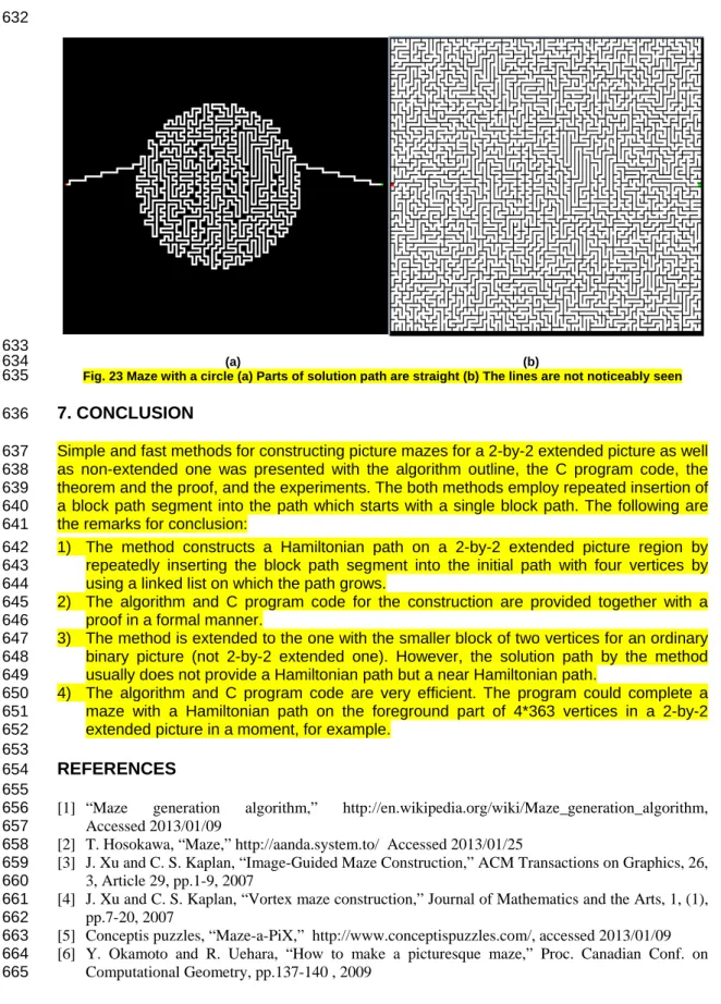
Some maze solution path segments were often seen before the maze was solved in the 624

paper [12]. However, this problem is not noticeably seen in the experimental results of this 625

study. The horizontal, vertical or near 45 degree straight lines were often seen before the 626

solution was made. These horizontal straight lines are avoided with some zigzags in Fig. 14. 627

Another maze was constructed in Fig. 23. The straight lines were drawn with some slopes 628

but not around 45 degree or near vertical or horizontal. Those lines are not noticeably seen 629

in Fig. 23 (b), which is a completed maze with walls thinned. 630

632

633

(a) (b) 634

Fig. 23 Maze with a circle (a) Parts of solution path are straight (b) The lines are not noticeably seen 635

7. CONCLUSION

Simple and fast methods for constructing picture mazes for a 2-by-2 extended picture as well 637

as non-extended one was presented with the algorithm outline, the C program code, the 638

theorem and the proof, and the experiments. The both methods employ repeated insertion of 639

a block path segment into the path which starts with a single block path. The following are 640

the remarks for conclusion: 641

1) The method constructs a Hamiltonian path on a 2-by-2 extended picture region by 642

repeatedly inserting the block path segment into the initial path with four vertices by 643

using a linked list on which the path grows. 644

2) The algorithm and C program code for the construction are provided together with a 645

proof in a formal manner. 646

3) The method is extended to the one with the smaller block of two vertices for an ordinary 647

binary picture (not 2-by-2 extended one). However, the solution path by the method 648

usually does not provide a Hamiltonian path but a near Hamiltonian path. 649

4) The algorithm and C program code are very efficient. The program could complete a 650

maze with a Hamiltonian path on the foreground part of 4*363 vertices in a 2-by-2 651

extended picture in a moment, for example. 652

653

REFERENCES

655

[1] “Maze generation algorithm,” http://en.wikipedia.org/wiki/Maze_generation_algorithm,

656

Accessed 2013/01/09

657

[2] T. Hosokawa, “Maze,” http://aanda.system.to/ Accessed 2013/01/25

658

[3] J. Xu and C. S. Kaplan, “Image-Guided Maze Construction,” ACM Transactions on Graphics, 26,

659

3, Article 29, pp.1-9, 2007

660

[4] J. Xu and C. S. Kaplan, “Vortex maze construction,” Journal of Mathematics and the Arts, 1, (1),

661

pp.7-20, 2007

662

[5] Conceptis puzzles, “Maze-a-PiX,” http://www.conceptispuzzles.com/, accessed 2013/01/09

663

[6] Y. Okamoto and R. Uehara, “How to make a picturesque maze,” Proc. Canadian Conf. on

664

Computational Geometry, pp.137-140 , 2009

[7] H. Hamada, http://www.lab2.kuis.kyoto-u.ac.jp/~itohiro/Games/100301/100301-11.pdf ,

666

accessed 20013/01/12

667

[8] K. Hamada, “A Picturesque Maze Generation Algorithm with Any Given Endpoints,” Journal of

668

Information Processing, Vol. 21, No. 3, pp.393-397, 2013

669

[9] K. Ikeda and J. Hashimoto, “Stochastic Optimization for Picture Maze Generation,” Jouhou Shori

670

Gakkai Ronbunshi, Vol. 53, No.6, pp.1625-2634, 2012, in Japanese

671

[10]T. Kurokawa, K. Mori, and T. Mizuno, ”Automatic construction of picture maze by repeated

672

contour connection,” Thailand-Japan Joint Conference on Computational Geometry and Graphs,

673

pp.5-6, 2012

674

[11]T. Kurokawa, “Picture maze generation and its relation to graphs,” 2013 SHIKOKU-SECTION

675

JOINT CONVENTION RECORD OF THE INSTITUTE OF ELECTRICAL AND RELATED

676

ENGINEERS, p.231, 2013

677

[12]T. Kurokawa, ”Picture Maze Generation by Repeated Contour Connection and Graph Structure

678

of Maze,” Computer Science and Engineering, Vol.3, No.3, pp.76-83, 2013.12, Scientific &

679

Academic Publishing, USA , ISSN:2163-1484

680

http://article.sapub.org/10.5923.j.computer.20130303.04.html Accessed 2014/1/20

681

[13]F. J. Wong and S. Takahashi, “Flow-based Automatic Generation of Hybrid Picture Mazes,”

682

Computer Graphics Forum, 28, (7), pp.1975-1984, Wiley-Blackwell, 2009

683

[14]S. Ishida, "Algorithm of automatic maze generation,"

684

http://www5d.biglobe.ne.jp/%257estssk/maze/make.html, (Japanese), Accessed 2013/10/8

685

[15]“How to Build a Maze,” http://www.mazeworks.com/mazegen/mazetut/index.htm, Accessed

686

2013/1/26

687

[16]http://www.microsoft.com/ja-jp/dev/express/default.aspx, Accessed 2012/10/15

688

[17]http://jaist.dl.sourceforge.net/project/opencvlibrary/opencv-win/2.1/ Accessed Oct., 2011

689 690