Visit :

(1)

Visit :

https://hemanthrajhemu.github.io

Join Telegram to get Instant Updates:

https://bit.ly/VTU_TELEGRAM

Contact: MAIL:

[email protected]

INSTAGRAM:

www.instagram.com/hemanthraj_hemu/

INSTAGRAM:

www.instagram.com/futurevisionbie/

(2)

5.2 ANALOG-TO-ANALOG CONVERSION

147

5.2.1 Amplitude Modulation (AM) 147 5.2.2 Frequency Modulation (FM) 148 5.2.3 Phase Modulation (PM) 149

5.3 END-CHAPTER MATERIALS

151

5.3.1 Recommended Reading 151 5.3.2 Key Terms 151 5.3.3 Summary 151

5.4 PRACTICE SET

152

5.4.1 Quizzes 152 5.4.2 Questions 152 5.4.3 Problems 153

5.5 SIMULATION EXPERIMENTS

154

5.5.1 Applets 154

Chapter 6 Bandwidth Utilization: Multiplexing and Spectrum

Spreading

155

6.1 MULTIPLEXING

156

6.1.1 Frequency-Division Multiplexing 157 6.1.2 Wavelength-Division Multiplexing 162 6.1.3 Time-Division Multiplexing 163

6.2 SPREAD SPECTRUM

175

6.2.1 Frequency Hopping Spread Spectrum 176 6.2.2 Direct Sequence Spread Spectrum 178

6.3 END-CHAPTER MATERIALS

180

6.4 PRACTICE SET

181

6.5 SIMULATION EXPERIMENTS

184

6.5.1 Applets 184

Chapter 7 Transmission Media

185

7.1 INTRODUCTION

186

7.2 GUIDED MEDIA

187

7.2.1 Twisted-Pair Cable 187 7.2.2 Coaxial Cable 190 7.2.3 Fiber-Optic Cable 192

7.3 UNGUIDED MEDIA: WIRELESS

197

7.3.1 Radio Waves 199 7.3.2 Microwaves 200 7.3.3 Infrared 201

(3)

7.4 END-CHAPTER MATERIALS

202

7.5 PRACTICE SET

203

Chapter 8 Switching

207

8.1 INTRODUCTION

208

8.1.1 Three Methods of Switching 208 8.1.2 Switching and TCP/IP Layers 209

8.2 CIRCUIT-SWITCHED NETWORKS

209

8.2.1 Three Phases 211 8.2.2 Efficiency 212 8.2.3 Delay 213

8.3 PACKET SWITCHING

213

8.3.1 Datagram Networks 214 8.3.2 Virtual-Circuit Networks 216

8.4 STRUCTURE OF A SWITCH

222

8.4.1 Structure of Circuit Switches 222 8.4.2 Structure of Packet Switches 226

8.5 END-CHAPTER MATERIALS

230

8.5.1 Recommended Reading 230 8.5.2 Key terms 230 8.5.3 Summary 230

8.6 PRACTICE SET

231

8.7 SIMULATION EXPERIMENTS

234

8.7.1 Applets 234

PART III: Data-Link Layer

235

Chapter 9 Introduction to Data-Link Layer

237

9.1 INTRODUCTION

238

9.1.1 Nodes and Links 239 9.1.2 Services 239

9.1.3 Two Categories of Links 241 9.1.4 Two Sublayers 242

9.2 LINK-LAYER ADDRESSING

242

9.2.1 Three Types of addresses 244

9.2.2 Address Resolution Protocol (ARP) 245 9.2.3 An Example of Communication 248

(4)

9.3 END-CHAPTER MATERIALS

252

9.4 PRACTICE SET

253

Chapter 10 Error Detection and Correction

257

10.1 INTRODUCTION

258

10.1.1 Types of Errors 258 10.1.2 Redundancy 258

10.1.3 Detection versus Correction 258 10.1.4 Coding 259

10.2 BLOCK CODING

259

10.2.1 Error Detection 259

10.3 CYCLIC CODES

264

10.3.1 Cyclic Redundancy Check 264 10.3.2 Polynomials 267

10.3.3 Cyclic Code Encoder Using Polynomials 269 10.3.4 Cyclic Code Analysis 270

10.3.5 Advantages of Cyclic Codes 274 10.3.6 Other Cyclic Codes 274 10.3.7 Hardware Implementation 274

10.4 CHECKSUM

277

10.4.1 Concept 278

10.4.2 Other Approaches to the Checksum 281

10.5 FORWARD ERROR CORRECTION

282

10.5.1 Using Hamming Distance 283 10.5.2 Using XOR 283

10.5.3 Chunk Interleaving 283

10.5.4 Combining Hamming Distance and Interleaving 284 10.5.5 Compounding High- and Low-Resolution Packets 284

10.6 END-CHAPTER MATERIALS

285

10.7 PRACTICE SET

287

10.8 SIMULATION EXPERIMENTS

292

10.8.1 Applets 292

10.9 PROGRAMMING ASSIGNMENTS

292 https://hemanthrajhemu.github.io

(5)

155

B

andwidth Utilization:

Multiplexing and

Spectrum Spreading

n real life, we have links with limited bandwidths. The wise use of these bandwidths has been, and will be, one of the main challenges of electronic communications. However, the meaning of wise may depend on the application. Sometimes we need to combine several low-bandwidth channels to make use of one channel with a larger bandwidth. Sometimes we need to expand the bandwidth of a channel to achieve goals such as privacy and antijamming. In this chapter, we explore these two broad categories of bandwidth utilization: multiplexing and spectrum spreading. In multiplexing, our goal is efficiency; we combine several channels into one. In spectrum spreading, our goals are privacy and antijamming; we expand the bandwidth of a channel to insert redundancy, which is necessary to achieve these goals.

This chapter is divided into two sections:

❑ The first section discusses multiplexing. The first method described in this section is called frequency-division multiplexing (FDM), which means to combine several analog signals into a single analog signal. The second method is called wavelength-division multiplexing (WDM), which means to combine several optical signals into one optical signal.The third method is called time-division multiplexing (TDM), which allows several digital signals to share a channel in time.

❑ The second section discusses spectrum spreading, in which we first spread the band-width of a signal to add redundancy for the purpose of more secure transmission before combining different channels. The first method described in this section is called frequency hopping spread spectrum (FHSS), in which different modulation frequencies are used in different periods of time. The second method is called direct sequence spread spectrum (DSSS), in which a single bit in the original signal is changed to a sequence before transmission.

I

(6)

6.1 MU

L

TIP

LE

XI

NG

Whenever the bandwidth of a medium linking two devices is greater than the band-width needs of the devices, the link can be shared. Multiplexing is the set of techniques that allow the simultaneous transmission of multiple signals across a single data link. As data and telecommunications use increases, so does traffic. We can accommodate this increase by continuing to add individual links each time a new channel is needed; or we can install higher-bandwidth links and use each to carry multiple signals. As described in Chapter 7, today’s technology includes high-bandwidth media such as optical fiber and terrestrial and satellite microwaves. Each has a bandwidth far in excess of that needed for the average transmission signal. If the bandwidth of a link is greater than the bandwidth needs of the devices connected to it, the bandwidth is wasted. An efficient system maximizes the utilization of all resources; bandwidth is one of the most precious resources we have in data communications.

In a multiplexed system, n lines share the bandwidth of one link. Figure 6.1 shows the basic format of a multiplexed system. The lines on the left direct their transmission streams to a multiplexer (MUX), which combines them into a single stream (many-to-one). At the receiving end, that stream is fed into a demultiplexer (DEMUX), which separates the stream back into its component transmissions (one-to-many) and directs them to their corresponding lines. In the figure, the word link refers to the physical path. The word channel refers to the portion of a link that carries a transmis-sion between a given pair of lines. One link can have many (n) channels.

There are three basic multiplexing techniques: frequency-division multiplexing, wavelength-division multiplexing, and time-division multiplexing. The first two are techniques designed for analog signals, the third, for digital signals (see Figure 6.2). Figure 6.1 Dividing a link into channels

Figure 6.2 Categories of multiplexing

1 link, n channels n Input lines n Output lines MUX: Multiplexer DEMUX: Demultiplexer M U X D E M U X • • • • • • Multiplexing Frequency-division multiplexing Analog Wavelength-division multiplexing Analog Time-division multiplexing Digital

https://hemanthrajhemu.github.io

(7)

Although some textbooks consider carrier division multiple access (CDMA) as a fourth multiplexing category, we discuss CDMA as an access method (see Chapter 12).

6.1.1 Frequency-

D

ivision Multiplexing

Frequency-division multiplexing (FDM) is an analog technique that can be applied when the bandwidth of a link (in hertz) is greater than the combined bandwidths of the signals to be transmitted. In FDM, signals generated by each sending device modu-late different carrier frequencies. These modumodu-lated signals are then combined into a single composite signal that can be transported by the link. Carrier frequencies are separated by sufficient bandwidth to accommodate the modulated signal. These bandwidth ranges are the channels through which the various signals travel. Channels can be sepa-rated by strips of unused bandwidth—guard bands—to prevent signals from overlap-ping. In addition, carrier frequencies must not interfere with the original data frequencies.

Figure 6.3 gives a conceptual view of FDM. In this illustration, the transmission path is divided into three parts, each representing a channel that carries one transmission.

We consider FDM to be an analog multiplexing technique; however, this does not mean that FDM cannot be used to combine sources sending digital signals. A digital signal can be converted to an analog signal (with the techniques discussed in Chapter 5) before FDM is used to multiplex them.

Multiplexing Process

Figure 6.4 is a conceptual illustration of the multiplexing process. Each source gener-ates a signal of a similar frequency range. Inside the multiplexer, these similar signals modulate different carrier frequencies (f₁, f₂,and f₃). The resulting modulated signals are then combined into a single composite signal that is sent out over a media link that has enough bandwidth to accommodate it.

Figure 6.3 Frequency-division multiplexing

FDM is an analog multiplexing technique that combines analog signals.

Channel 1

Input

lines Channel 2 Outputlines

Channel 3 M U X D E M U X

https://hemanthrajhemu.github.io

(8)

Demultiplexing Process

The demultiplexer uses a series of filters to decompose the multiplexed signal into its constituent component signals. The individual signals are then passed to a demodulator that separates them from their carriers and passes them to the output lines. Figure 6.5 is a conceptual illustration of demultiplexing process.

Example 6.1

Assume that a voice channel occupies a bandwidth of 4 kHz. We need to combine three voice channels into a link with a bandwidth of 12 kHz, from 20 to 32 kHz. Show the configuration, using the frequency domain. Assume there are no guard bands.

Solution

We shift (modulate) each of the three voice channels to a different bandwidth, as shown in Fig-ure 6.6. We use the 20- to 24-kHz bandwidth for the first channel, the 24- to 28-kHz bandwidth

Figure 6.4 FDM process

Figure 6.5 FDM demultiplexing example

+ Modulator Carrier f2 Modulator Carrier f3 Modulator Carrier f1 Baseband analog signals Demodulator Carrier f1 Demodulator Carrier f₂ Demodulator Carrier f3 Filter Filter

Filter _{analog signals}Baseband

(9)

for the second channel, and the 28- to 32-kHz bandwidth for the third one. Then we combine them as shown in Figure 6.6. At the receiver, each channel receives the entire signal, using a filter to separate out its own signal. The first channel uses a filter that passes frequencies between 20 and 24 kHz and filters out (discards) any other frequencies. The second channel uses a filter that passes frequencies between 24 and 28 kHz, and the third channel uses a filter that passes frequencies between 28 and 32 kHz. Each channel then shifts the frequency to start from zero.

Example 6.2

Five channels, each with a 100-kHz bandwidth, are to be multiplexed together. What is the mini-mum bandwidth of the link if there is a need for a guard band of 10 kHz between the channels to prevent interference?

Solution

For five channels, we need at least four guard bands. This means that the required bandwidth is at least 5 × 100 + 4 × 10 = 540 kHz, as shown in Figure 6.7.

Example 6.3

Four data channels (digital), each transmitting at 1 Mbps, use a satellite channel of 1 MHz. Design an appropriate configuration, using FDM.

Solution

The satellite channel is analog. We divide it into four channels, each channel having a 250-kHz bandwidth. Each digital channel of 1 Mbps is modulated so that each 4 bits is modulated to 1 Hz. One solution is 16-QAM modulation. Figure 6.8 shows one possible configuration.

Figure 6.6 Example 6.1 0 4 0 4 0 4 20 24 24 28 28 32 20 32 20 32 Higher-bandwidth link 0 4 0 4 0 4 20 24 24 28 28 32 Filter and shift

Shift and combine

Bandpass filter Bandpass filter Bandpass filter Modulator Modulator Modulator +

https://hemanthrajhemu.github.io

(10)

The Analog Carrier System

To maximize the efficiency of their infrastructure, telephone companies have tradition-ally multiplexed signals from lower-bandwidth lines onto higher-bandwidth lines. In this way, many switched or leased lines can be combined into fewer but bigger chan-nels. For analog lines, FDM is used.

One of these hierarchical systems used by telephone companies is made up of groups, supergroups, master groups, and jumbo groups (see Figure 6.9).

In this analog hierarchy, 12 voice channels are multiplexed onto a higher-bandwidth line to create a group. A group has 48 kHz of bandwidth and supports 12 voice channels. At the next level, up to five groups can be multiplexed to create a composite signal called a supergroup. A supergroup has a bandwidth of 240 kHz and supports up to 60 voice channels. Supergroups can be made up of either five groups or 60 independent voice channels.

At the next level, 10 supergroups are multiplexed to create a master group. A master group must have 2.40 MHz of bandwidth, but the need for guard bands between the supergroups increases the necessary bandwidth to 2.52 MHz. Master groups support up to 600 voice channels.

Finally, six master groups can be combined into a jumbo group. A jumbo group must have 15.12 MHz (6 × 2.52 MHz) but is augmented to 16.984 MHz to allow for guard bands between the master groups.

Figure 6.7 Example 6.2 Figure 6.8 Example 6.3 100 kHz 100 kHz 100 kHz 100 kHz 100 kHz 540 kHz Guard band of 10 kHz 1 MHz 1 Mbps Digital 16-QAM 1 Mbps Digital 16-QAM 1 Mbps Digital 16-QAM 1 Mbps Digital Analog 250 kHz Analog 250 kHz Analog 250 kHz Analog 250 kHz 16-QAM FDM

https://hemanthrajhemu.github.io

(11)

Other Applications of FDM

A very common application of FDM is AM and FM radio broadcasting. Radio uses the air as the transmission medium. A special band from 530 to 1700 kHz is assigned to AM radio. All radio stations need to share this band. As discussed in Chapter 5, each AM station needs 10 kHz of bandwidth. Each station uses a different carrier frequency, which means it is shifting its signal and multiplexing. The signal that goes to the air is a combination of signals. A receiver receives all these signals, but filters (by tuning) only the one which is desired. Without multiplexing, only one AM station could broadcast to the common link, the air. However, we need to know that there is no physical multi-plexer or demultimulti-plexer here. As we will see in Chapter 12, multiplexing is done at the data-link layer.

The situation is similar in FM broadcasting. However, FM has a wider band of 88 to 108 MHz because each station needs a bandwidth of 200 kHz.

Another common use of FDM is in television broadcasting. Each TV channel has its own bandwidth of 6 MHz.

The first generation of cellular telephones (See Chapter 16) also uses FDM. Each user is assigned two 30-kHz channels, one for sending voice and the other for receiv-ing. The voice signal, which has a bandwidth of 3 kHz (from 300 to 3300 Hz), is mod-ulated by using FM. Remember that an FM signal has a bandwidth 10 times that of the modulating signal, which means each channel has 30 kHz (10 × 3) of bandwidth. Therefore, each user is given, by the base station, a 60-kHz bandwidth in a range avail-able at the time of the call.

Example 6.4

The Advanced Mobile Phone System (AMPS) uses two bands. The first band of 824 to 849 MHz is used for sending, and 869 to 894 MHz is used for receiving. Each user has a bandwidth of 30 kHz in each direction. The 3-kHz voice is modulated using FM, creating 30 kHz of modulated signal. How many people can use their cellular phones simultaneously?

Figure 6.9 Analog hierarchy

Jumbo group 6 Master group 10 Supergroup 5 Group F D M F D M F D M _F D M 4 kHz 4 kHz 4 kHz 12 v oice channels • • • • • • 16.984 MHz 3600 voice channels 2.52 MHz 600 voice channels 48 kHz 12 voice channels 240 kHz 60 voice channels

https://hemanthrajhemu.github.io

(12)

Solution

Each band is 25 MHz. If we divide 25 MHz by 30 kHz, we get 833.33. In reality, the band is divided into 832 channels. Of these, 42 channels are used for control, which means only 790 channels are available for cellular phone users. We discuss AMPS in greater detail in Chapter 16.

Implementation

FDM can be implemented very easily. In many cases, such as radio and television broadcasting, there is no need for a physical multiplexer or demultiplexer. As long as the stations agree to send their broadcasts to the air using different carrier frequencies, multiplexing is achieved. In other cases, such as the cellular telephone system, a base station needs to assign a carrier frequency to the telephone user. There is not enough bandwidth in a cell to permanently assign a bandwidth range to every telephone user. When a user hangs up, her or his bandwidth is assigned to another caller.

6.1.2 Wavelength-

D

ivision Multiplexing

Wavelength-division multiplexing (WDM) is designed to use the high-data-rate capability of fiber-optic cable. The optical fiber data rate is higher than the data rate of metallic transmission cable, but using a fiber-optic cable for a single line wastes the available bandwidth. Multiplexing allows us to combine several lines into one.

WDM is conceptually the same as FDM, except that the multiplexing and demulti-plexing involve optical signals transmitted through fiber-optic channels. The idea is the same: We are combining different signals of different frequencies. The difference is that the frequencies are very high.

Figure 6.10 gives a conceptual view of a WDM multiplexer and demultiplexer. Very narrow bands of light from different sources are combined to make a wider band of light. At the receiver, the signals are separated by the demultiplexer.

Although WDM technology is very complex, the basic idea is very simple. We want to combine multiple light sources into one single light at the multiplexer and do the reverse at the demultiplexer. The combining and splitting of light sources are easily handled by a prism. Recall from basic physics that a prism bends a beam of light based on the angle of incidence and the frequency. Using this technique, a multiplexer can be Figure 6.10 Wavelength-division multiplexing

WDM is an analog multiplexing technique to combine optical signals.

λ1 λ3 λ2 M U X D E M U X λ1 λ3 λ2 λ1 + λ2 + λ3

https://hemanthrajhemu.github.io

(13)

made to combine several input beams of light, each containing a narrow band of frequencies, into one output beam of a wider band of frequencies. A demultiplexer can also be made to reverse the process. Figure 6.11 shows the concept.

One application of WDM is the SONET network, in which multiple optical fiber lines are multiplexed and demultiplexed. We discuss SONET in Chapter 14.

A new method, called dense WDM(DWDM), can multiplex a very large number of channels by spacing channels very close to one another. It achieves even greater efficiency.

6.1.3 Time-

D

ivision Multiplexing

Time-division multiplexing (TDM) is a digital process that allows several connections to share the high bandwidth of a link. Instead of sharing a portion of the bandwidth as in FDM, time is shared. Each connection occupies a portion of time in the link. Figure 6.12 gives a conceptual view of TDM. Note that the same link is used as in FDM; here, how-ever, the link is shown sectioned by time rather than by frequency. In the figure, portions of signals 1, 2, 3, and 4 occupy the link sequentially.

Note that in Figure 6.12 we are concerned with only multiplexing, not switching. This means that all the data in a message from source 1 always go to one specific desti-nation, be it 1, 2, 3, or 4. The delivery is fixed and unvarying, unlike switching.

We also need to remember that TDM is, in principle, a digital multiplexing technique. Digital data from different sources are combined into one timeshared link. However, this Figure 6.11 Prisms in wavelength-division multiplexing and demultiplexing

Figure 6.12 TDM Demultiplexer Fiber-optic cable Multiplexer λ1 λ2 λ3 λ1 λ1 + λ2 + λ3 λ2 λ3 1 1 1 2 2 2 3 3 3 4 4 4 1 2 3 4 1 2 3 4 M U X Data flow D E M U X

https://hemanthrajhemu.github.io

(14)

does not mean that the sources cannot produce analog data; analog data can be sampled, changed to digital data, and then multiplexed by using TDM.

We can divide TDM into two different schemes: synchronous and statistical. We first discuss synchronous TDM and then show how statistical TDM differs.

Synchronous TDM

In synchronous TDM, each input connection has an allotment in the output even if it is not sending data.

Time Slots and Frames

In synchronous TDM, the data flow of each input connection is divided into units, where each input occupies one input time slot. A unit can be 1 bit, one character, or one block of data. Each input unit becomes one output unit and occupies one output time slot. However, the duration of an output time slot is n times shorter than the duration of an input time slot. If an input time slot is T s, the output time slot is T/n s, where n is the number of connections. In other words, a unit in the output connection has a shorter duration; it travels faster. Figure 6.13 shows an example of synchronous TDM where n

is 3.

In synchronous TDM, a round of data units from each input connection is collected into a frame (we will see the reason for this shortly). If we have n connections, a frame is divided into n time slots and one slot is allocated for each unit, one for each input line. If the duration of the input unit is T, the duration of each slot is T/n and the dura-tion of each frame is T (unless a frame carries some other information, as we will see shortly).

The data rate of the output link must be ntimes the data rate of a connection to guarantee the flow of data. In Figure 6.13, the data rate of the link is 3 times the data rate of a connection; likewise, the duration of a unit on a connection is 3 times that of

TDM is a digital multiplexing technique for combining several low-rate channels into one high-rate one.

Figure 6.13 Synchronous time-division multiplexing

Frame 1 A1 C1 B1 Frame 2 A2 C2 B2 Frame 3 A3 C3 B3

Each frame is 3 time slots. Each time slot duration is T/3 s.

Data are taken from each line every T s. A1 C1 B1 T A2 B2 C2 T A3 B3 C3 T T T/3 FDMMUX

https://hemanthrajhemu.github.io

(15)

the time slot (duration of a unit on the link). In the figure we represent the data prior to multiplexing as 3 times the size of the data after multiplexing. This is just to convey the idea that each unit is 3 times longer in duration before multiplexing than after.

Time slots are grouped into frames. A frame consists of one complete cycle of time slots, with one slot dedicated to each sending device. In a system with n input lines, each frame has n slots, with each slot allocated to carrying data from a specific input line.

Example 6.5

In Figure 6.13, the data rate for each input connection is 1 kbps. If 1 bit at a time is multiplexed (a unit is 1 bit), what is the duration of

1. each input slot, 2. each output slot, and 3. each frame? Solution

We can answer the questions as follows:

1. The data rate of each input connection is 1 kbps. This means that the bit duration is 1/1000 s or 1 ms. The duration of the input time slot is 1 ms (same as bit duration).

2. The duration of each output time slot is one-third of the input time slot. This means that the duration of the output time slot is 1/3 ms.

3. Each frame carries three output time slots. So the duration of a frame is 3 × 1/3 ms, or 1 ms. The duration of a frame is the same as the duration of an input unit.

Example 6.6

Figure 6.14 shows synchronous TDM with a data stream for each input and one data stream for the output. The unit of data is 1 bit. Find (1) the input bit duration, (2) the output bit duration, (3) the output bit rate, and (4) the output frame rate.

Solution

1. The input bit duration is the inverse of the bit rate: 1/1 Mbps = 1 μs. 2. The output bit duration is one-fourth of the input bit duration, or 1/4 μs.

In synchronous TDM, the data rate of the link is n times faster, and the unit duration is n times shorter.

Figure 6.14 Example 6.6 1 1 1 1 1 0 0 0 0 0 1 0 1 0 1 0 0 1 0 0 Frames 1 Mbps 1 Mbps 1 Mbps 1 Mbps • • • • • • • • • • • • • • • 0 1 0 10 0 0 1 1 1 0 1 0 0 0 1 0 1 0 1 MUX

https://hemanthrajhemu.github.io

(16)

3. The output bit rate is the inverse of the output bit duration, or 1/4 μs, or 4 Mbps. This can also be deduced from the fact that the output rate is 4 times as fast as any input rate; so the output rate = 4 × 1 Mbps = 4 Mbps.

4. The frame rate is always the same as any input rate. So the frame rate is 1,000,000 frames per second. Because we are sending 4 bits in each frame, we can verify the result of the pre-vious question by multiplying the frame rate by the number of bits per frame.

Example 6.7

Four 1-kbps connections are multiplexed together. A unit is 1 bit. Find (1) the duration of 1 bit before multiplexing, (2) the transmission rate of the link, (3) the duration of a time slot, and (4) the duration of a frame.

Solution

1. The duration of 1 bit before multiplexing is 1/1 kbps, or 0.001 s (1 ms). 2. The rate of the link is 4 times the rate of a connection, or 4 kbps.

3. The duration of each time slot is one-fourth of the duration of each bit before multiplexing, or 1/4 ms or 250 μs. Note that we can also calculate this from the data rate of the link, 4 kbps. The bit duration is the inverse of the data rate, or 1/4 kbps or 250 μs.

4. The duration of a frame is always the same as the duration of a unit before multiplexing, or 1 ms. We can also calculate this in another way. Each frame in this case has four time slots. So the duration of a frame is 4 times 250 μs, or 1 ms.

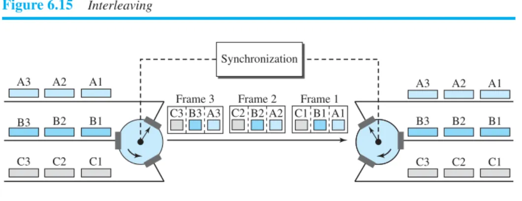
Interleaving

TDM can be visualized as two fast-rotating switches, one on the multiplexing side and the other on the demultiplexing side. The switches are synchronized and rotate at the same speed, but in opposite directions. On the multiplexing side, as the switch opens in front of a connection, that connection has the opportunity to send a unit onto the path. This process is called interleaving. On the demultiplexing side, as the switch opens in front of a connection, that connection has the opportunity to receive a unit from the path.

Figure 6.15 shows the interleaving process for the connection shown in Figure 6.13. In this figure, we assume that no switching is involved and that the data from the first connection at the multiplexer site go to the first connection at the demultiplexer. We discuss switching in Chapter 8.

Example 6.8

Four channels are multiplexed using TDM. If each channel sends 100 bytes/s and we multiplex 1 byte per channel, show the frame traveling on the link, the size of the frame, the duration of a frame, the frame rate, and the bit rate for the link.

Solution

The multiplexer is shown in Figure 6.16. Each frame carries 1 byte from each channel; the size of each frame, therefore, is 4 bytes, or 32 bits. Because each channel is sending 100 bytes/s and a frame carries 1 byte from each channel, the frame rate must be 100 frames per second. The

(17)

duration of a frame is therefore 1/100 s. The link is carrying 100 frames per second, and since each frame contains 32 bits, the bit rate is 100 × 32, or 3200 bps. This is actually 4 times the bit rate of each channel, which is 100 × 8 = 800 bps.

Example 6.9

A multiplexer combines four 100-kbps channels using a time slot of 2 bits. Show the output with four arbitrary inputs. What is the frame rate? What is the frame duration? What is the bit rate? What is the bit duration?

Solution

Figure 6.17 shows the output for four arbitrary inputs. The link carries 50,000 frames per second since each frame contains 2 bits per channel. The frame duration is therefore 1/50,000 s or 20 μs. The frame rate is 50,000 frames per second, and each frame carries 8 bits; the bit rate is 50,000 × 8 = 400,000 bits or 400 kbps. The bit duration is 1/400,000 s, or 2.5 μs. Note that the frame dura-tion is 8 times the bit duradura-tion because each frame is carrying 8 bits.

Empty Slots

Synchronous TDM is not as efficient as it could be. If a source does not have data to send, the corresponding slot in the output frame is empty. Figure 6.18 shows a case in which one of the input lines has no data to send and one slot in another input line has discontinuous data.

The first output frame has three slots filled, the second frame has two slots filled, and the third frame has three slots filled. No frame is full. We learn in the next section

Figure 6.15 Interleaving Figure 6.16 Example 6.8 Frame 1 A1 C1 Frame 2 A2 B2 B1 Frame 3 A3 B3 C3 C2 A3 A2 A1 C1 C2 C3 B2 B1 B3 A3 A2 A1 C1 C3 C2 B2 B1 B3 Synchronization MUX 100 bytes/s Frame 4 bytes 32 bits • • • Frame 4 bytes 32 bits 100 frames/s 3200 bps Frame duration = s 1 100

https://hemanthrajhemu.github.io

(18)

that statistical TDM can improve the efficiency by removing the empty slots from the frame.

Data Rate Management

One problem with TDM is how to handle a disparity in the input data rates. In all our discussion so far, we assumed that the data rates of all input lines were the same. However, if data rates are not the same, three strategies, or a combination of them, can be used. We call these three strategies multilevel multiplexing, multiple-slot allocation, and

pulse stuffing.

Multilevel Multiplexing Multilevel multiplexing is a technique used when the data rate of an input line is a multiple of others. For example, in Figure 6.19, we have two inputs of 20 kbps and three inputs of 40 kbps. The first two input lines can be multiplexed together to provide a data rate equal to the last three. A second level of multiplexing can create an output of 160 kbps.

Figure 6.17 Example 6.9

Figure 6.18 Empty slots

Figure 6.19 Multilevel multiplexing

100 kbps 100 kbps 100 kbps 100 kbps

Frame: 8 bits Frame: 8 bits Frame: 8 bits

50,000 frames/s 400 kbps Frame duration = 1/50,000 s = 20 μs 1 1 0 0 1 0 0 0 0 1 1 1 1 0 1 1 0 1 0 0 1 0 1 0 _{• • •} ₀₀ ₁₀ ₀₀ ₁₁ ₀₁ ₁₁ ₁₀ ₀₀ ₁₁ ₀₁ ₁₀ ₁₀ MUX • • • • • • • • • • • • MUX 40 kbps 40 kbps 40 kbps 40 kbps 160 kbps 20 kbps 20 kbps MUX

https://hemanthrajhemu.github.io

(19)

Multiple-Slot Allocation Sometimes it is more efficient to allot more than one slot in a frame to a single input line. For example, we might have an input line that has a data rate that is a multiple of another input. In Figure 6.20, the input line with a 50-kbps data rate can be given two slots in the output. We insert a demultiplexer in the line to make two inputs out of one.

Pulse Stuffing Sometimes the bit rates of sources are not multiple integers of each other. Therefore, neither of the above two techniques can be applied. One solution is to make the highest input data rate the dominant data rate and then add dummy bits to the input lines with lower rates. This will increase their rates. This technique is called pulse stuffing,bit padding, or bit stuffing. The idea is shown in Figure 6.21. The input with a data rate of 46 is pulse-stuffed to increase the rate to 50 kbps. Now multiplexing can take place.

Frame Synchronizing

The implementation of TDM is not as simple as that of FDM. Synchronization between the multiplexer and demultiplexer is a major issue. If the multiplexer and the demulti-plexer are not synchronized, a bit belonging to one channel may be received by the wrong channel. For this reason, one or more synchronization bits are usually added to the beginning of each frame. These bits, called framing bits, follow a pattern, frame to frame, that allows the demultiplexer to synchronize with the incoming stream so that it can separate the time slots accurately. In most cases, this synchronization information consists of 1 bit per frame, alternating between 0 and 1, as shown in Figure 6.22. Figure 6.20 Multiple-slot multiplexing

Figure 6.21 Pulse stuffing

125 kbps

The input with a 50-kHz data rate has two

slots in each frame.

25 kbps 25 kbps 25 kbps 25 kbps 25 kbps 50 kbps • • • M U X 46 kbps 150 kbps 50 kbps 50 kbps 50 kbps Pulse stuffing M U X

https://hemanthrajhemu.github.io

(20)

Example 6.10

We have four sources, each creating 250 characters per second. If the interleaved unit is a charac-ter and 1 synchronizing bit is added to each frame, find (1) the data rate of each source, (2) the duration of each character in each source, (3) the frame rate, (4) the duration of each frame, (5) the number of bits in each frame, and (6) the data rate of the link.

Solution

1. The data rate of each source is 250 × 8 = 2000 bps = 2 kbps.

2. Each source sends 250 characters per second; therefore, the duration of a character is 1/250 s, or 4 ms.

3. Each frame has one character from each source, which means the link needs to send 250 frames per second to keep the transmission rate of each source.

4. The duration of each frame is 1/250 s, or 4 ms. Note that the duration of each frame is the same as the duration of each character coming from each source.

5. Each frame carries 4 characters and 1 extra synchronizing bit. This means that each frame is 4 × 8 + 1 = 33 bits.

6. The link sends 250 frames per second, and each frame contains 33 bits. This means that the data rate of the link is 250 × 33, or 8250 bps. Note that the bit rate of the link is greater than the combined bit rates of the four channels. If we add the bit rates of four channels, we get 8000 bps. Because 250 frames are traveling per second and each contains 1 extra bit for synchronizing, we need to add 250 to the sum to get 8250 bps.

Example 6.11

Two channels, one with a bit rate of 100 kbps and another with a bit rate of 200 kbps, are to be multiplexed. How this can be achieved? What is the frame rate? What is the frame duration? What is the bit rate of the link?

Solution

We can allocate one slot to the first channel and two slots to the second channel. Each frame car-ries 3 bits. The frame rate is 100,000 frames per second because it carcar-ries 1 bit from the first channel. The frame duration is 1/100,000 s, or 10 ms. The bit rate is 100,000 frames/s × 3 bits per frame, or 300 kbps. Note that because each frame carries 1 bit from the first channel, the bit rate for the first channel is preserved. The bit rate for the second channel is also preserved because each frame carries 2 bits from the second channel.

Figure 6.22 Framing bits

Frame 1 Frame 2 Frame 3 A3 B3 C3 1 0 B2 A2 1 C1 A1 1 0 1 Synchronization pattern

https://hemanthrajhemu.github.io

(21)

Digital Signal Service

Telephone companies implement TDM through a hierarchy of digital signals, called

digital signal (DS) service or digital hierarchy. Figure 6.23 shows the data rates sup-ported by each level.

❑ DS-0 is a single digital channel of 64 kbps.

❑ DS-1 is a 1.544-Mbps service; 1.544 Mbps is 24 times 64 kbps plus 8 kbps of over-head. It can be used as a single service for 1.544-Mbps transmissions, or it can be used to multiplex 24 DS-0 channels or to carry any other combination desired by the user that can fit within its 1.544-Mbps capacity.

❑ DS-2 is a 6.312-Mbps service; 6.312 Mbps is 96 times 64 kbps plus 168 kbps of overhead. It can be used as a single service for 6.312-Mbps transmissions; or it can be used to multiplex 4 DS-1 channels, 96 DS-0 channels, or a combination of these service types.

❑ DS-3 is a 44.376-Mbps service; 44.376 Mbps is 672 times 64 kbps plus 1.368 Mbps of overhead. It can be used as a single service for 44.376-Mbps transmissions; or it can be used to multiplex 7 DS-2 channels, 28 DS-1 channels, 672 DS-0 channels, or a combination of these service types.

❑ DS-4 is a 274.176-Mbps service; 274.176 is 4032 times 64 kbps plus 16.128 Mbps of overhead. It can be used to multiplex 6 DS-3 channels, 42 DS-2 channels, 168 DS-1 channels, 4032 DS-0 channels, or a combination of these service types.

T Lines

DS-0, DS-1, and so on are the names of services. To implement those services, the tele-phone companies use T lines (T-1 to T-4). These are lines with capacities precisely matched to the data rates of the DS-1 to DS-4 services (see Table 6.1). So far only T-1 and T-3 lines are commercially available.

Figure 6.23 Digital hierarchy

T D M DS-0 24 • • • 64 kbps T D M DS-1 T D M T D M DS-4 DS-3 DS-2 _{274.176 Mbps} 6 DS-3 44.376 Mbps 7 DS-2 6.312 Mbps 4 DS-1 1.544 Mbps 24 DS-0

https://hemanthrajhemu.github.io

(22)

The T-1 line is used to implement DS-1; T-2 is used to implement DS-2; and so on. As you can see from Table 6.1, DS-0 is not actually offered as a service, but it has been defined as a basis for reference purposes.

T Lines for Analog Transmission

T lines are digital lines designed for the transmission of digital data, audio, or video. However, they also can be used for analog transmission (regular telephone connections), provided the analog signals are first sampled, then time-division multiplexed.

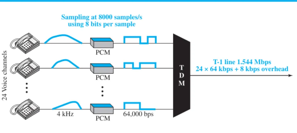
The possibility of using T lines as analog carriers opened up a new generation of services for the telephone companies. Earlier, when an organization wanted 24 separate telephone lines, it needed to run 24 twisted-pair cables from the company to the central exchange. (Remember those old movies showing a busy executive with 10 telephones lined up on his desk? Or the old office telephones with a big fat cable running from them? Those cables contained a bundle of separate lines.) Today, that same organization can combine the 24 lines into one T-1 line and run only the T-1 line to the exchange. Figure 6.24 shows how 24 voice channels can be multiplexed onto one T-1 line. (Refer to Chapter 4 for PCM encoding.)

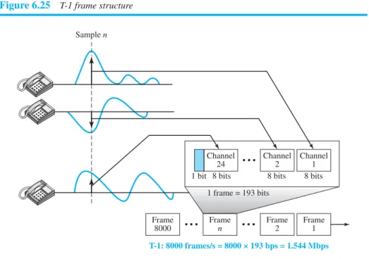
The T-1 Frame As noted above, DS-1 requires 8 kbps of overhead. To understand how this overhead is calculated, we must examine the format of a 24-voice-channel frame.

Table 6.1 DS and T line rates

Service Line Rate (Mbps) Voice Channels

DS-1 T-1 1.544 24

DS-2 T-2 6.312 96

DS-3 T-3 44.736 672

DS-4 T-4 274.176 4032

Figure 6.24 T-1 line for multiplexing telephone lines

T-1 line 1.544 Mbps 24 × 64 kbps + 8 kbps overhead 24 V oice channels T_D M 64,000 bps 4 kHz • • • • • • Sampling at 8000 samples/s using 8 bits per sample

PCM

(23)

The frame used on a T-1 line is usually 193 bits divided into 24 slots of 8 bits each plus 1 extra bit for synchronization (24 × 8 + 1 = 193); see Figure 6.25. In other words,

each slot contains one signal segment from each channel; 24 segments are interleaved in one frame. If a T-1 line carries 8000 frames, the data rate is 1.544 Mbps (193× 8000 = 1.544 Mbps)—the capacity of the line.

E Lines

Europeans use a version of T lines called E lines. The two systems are conceptually identical, but their capacities differ. Table 6.2 shows the E lines and their capacities.

More Synchronous TDM Applications

Some second-generation cellular telephone companies use synchronous TDM. For example, the digital version of cellular telephony divides the available bandwidth into 30-kHz bands. For each band, TDM is applied so that six users can share the band. This means that each 30-kHz band is now made of six time slots, and the digitized voice

Figure 6.25 T-1 frame structure

Table 6.2 E line rates

Line Rate (Mbps) Voice Channels

E-1 2.048 30 E-2 8.448 120 E-3 34.368 480 E-4 139.264 1920 8 bits Channel 1 1 bit 8 bits Channel 2 8 bits Channel 24 Frame

8000 Framen Frame2 Frame1

T-1: 8000 frames/s = 8000 × 193 bps = 1.544 Mbps 1 frame = 193 bits Sample n • • • • • • • • •

https://hemanthrajhemu.github.io

(24)

signals of the users are inserted in the slots. Using TDM, the number of telephone users in each area is now 6 times greater. We discuss second-generation cellular telephony in Chapter 16.

Statistical Time-Division Multiplexing

As we saw in the previous section, in synchronous TDM, each input has a reserved slot in the output frame. This can be inefficient if some input lines have no data to send. In statistical time-division multiplexing, slots are dynamically allocated to improve band-width efficiency. Only when an input line has a slot’s worth of data to send is it given a slot in the output frame. In statistical multiplexing, the number of slots in each frame is less than the number of input lines. The multiplexer checks each input line in round-robin fashion; it allocates a slot for an input line if the line has data to send; otherwise, it skips the line and checks the next line.

Figure 6.26 shows a synchronous and a statistical TDM example. In the former, some slots are empty because the corresponding line does not have data to send. In the latter, however, no slot is left empty as long as there are data to be sent by any input line.

Addressing

Figure 6.26 also shows a major difference between slots in synchronous TDM and sta-tistical TDM. An output slot in synchronous TDM is totally occupied by data; in statis-tical TDM, a slot needs to carry data as well as the address of the destination. In synchronous TDM, there is no need for addressing; synchronization and preassigned relationships between the inputs and outputs serve as an address. We know, for exam-ple, that input 1 always goes to input 2. If the multiplexer and the demultiplexer are synchronized, this is guaranteed. In statistical multiplexing, there is no fixed relation-ship between the inputs and outputs because there are no preassigned or reserved slots. We need to include the address of the receiver inside each slot to show where it is to be delivered. The addressing in its simplest form can be n bits to define N different output

Figure 6.26 TDM slot comparison

A1 B1 D1 1 B2 D2 E2 0 a. Synchronous TDM b. Statistical TDM A1 B1 B2 D1 D2 E2 Line A Line B Line C Line D Line E MUX MUX A1 B1 B2 D1 D2 E2 Line A Line B Line C Line D Line E B2 b D2 d E2 e dD1bB1 aA1

https://hemanthrajhemu.github.io

(25)

lines with n = log₂N. For example, for eight different output lines, we need a 3-bit address.

Slot Size

Since a slot carries both data and an address in statistical TDM, the ratio of the data size to address size must be reasonable to make transmission efficient. For example, it would be inefficient to send 1 bit per slot as data when the address is 3 bits. This would mean an overhead of 300 percent. In statistical TDM, a block of data is usually many bytes while the address is just a few bytes.

No Synchronization Bit

There is another difference between synchronous and statistical TDM, but this time it is at the frame level. The frames in statistical TDM need not be synchronized, so we do not need synchronization bits.

Bandwidth

In statistical TDM, the capacity of the link is normally less than the sum of the capaci-ties of each channel. The designers of statistical TDM define the capacity of the link based on the statistics of the load for each channel. If on average only x percent of the input slots are filled, the capacity of the link reflects this. Of course, during peak times, some slots need to wait.

6.2 SPR

E

A

D

SP

E

CTRUM

Multiplexing combines signals from several sources to achieve bandwidth efficiency; the available bandwidth of a link is divided between the sources. In spread spectrum (SS), we also combine signals from different sources to fit into a larger bandwidth, but our goals are somewhat different. Spread spectrum is designed to be used in wireless applications (LANs and WANs). In these types of applications, we have some concerns that outweigh bandwidth efficiency. In wireless applications, all stations use air (or a vacuum) as the medium for communication. Stations must be able to share this medium without interception by an eavesdropper and without being subject to jamming from a malicious intruder (in military operations, for example).

To achieve these goals, spread spectrum techniques add redundancy; they spread the original spectrum needed for each station. If the required bandwidth for each station is B, spread spectrum expands it to B_ss, such that B_ss>>B. The expanded bandwidth allows the source to wrap its message in a protective envelope for a more secure trans-mission. An analogy is the sending of a delicate, expensive gift. We can insert the gift in a special box to prevent it from being damaged during transportation, and we can use a superior delivery service to guarantee the safety of the package.

Figure 6.27 shows the idea of spread spectrum. Spread spectrum achieves its goals through two principles:

1. The bandwidth allocated to each station needs to be, by far, larger than what is needed. This allows redundancy.

(26)

2. The expanding of the original bandwidth B to the bandwidth B_ss must be done by a process that is independent of the original signal. In other words, the spreading process occurs after the signal is created by the source.

After the signal is created by the source, the spreading process uses a spreading code and spreads the bandwidth. The figure shows the original bandwidth B and the spread bandwidth B_SS. The spreading code is a series of numbers that look random, but are actually a pattern.

There are two techniques to spread the bandwidth: frequency hopping spread spec-trum (FHSS) and direct sequence spread specspec-trum (DSSS).

6.2.1 Frequency Hopping Spread Spectrum

The frequency hopping spread spectrum (FHSS) technique uses M different carrier frequencies that are modulated by the source signal. At one moment, the signal modu-lates one carrier frequency; at the next moment, the signal modumodu-lates another carrier frequency. Although the modulation is done using one carrier frequency at a time,

Mfrequencies are used in the long run. The bandwidth occupied by a source after spreading is B_FHSS >> B.

Figure 6.28 shows the general layout for FHSS. A pseudorandom code generator,

called pseudorandom noise (PN), creates a k-bit pattern for every hopping period T_h. The frequency table uses the pattern to find the frequency to be used for this hopping period and passes it to the frequency synthesizer. The frequency synthesizer creates a carrier signal of that frequency, and the source signal modulates the carrier signal.

Suppose we have decided to have eight hopping frequencies. This is extremely low for real applications and is just for illustration. In this case, M is 8 and k is 3. The pseudo-random code generator will create eight different 3-bit patterns. These are mapped to eight different frequencies in the frequency table (see Figure 6.29).

The pattern for this station is 101, 111, 001, 000, 010, 011, 100. Note that the pat-tern is pseudorandom; it is repeated after eight hoppings. This means that at hopping period 1, the pattern is 101. The frequency selected is 700 kHz; the source signal mod-ulates this carrier frequency. The second k-bit pattern selected is 111, which selects the 900-kHz carrier; the eighth pattern is 100, and the frequency is 600 kHz. After eight hoppings, the pattern repeats, starting from 101 again. Figure 6.30 shows how the signal

Figure 6.27 Spread spectrum

Spreading process B_SS B Spreading code

https://hemanthrajhemu.github.io

(27)

hops around from carrier to carrier. We assume the required bandwidth of the original signal is 100 kHz.

It can be shown that this scheme can accomplish the previously mentioned goals. If there are many k-bit patterns and the hopping period is short, a sender and receiver can have privacy. If an intruder tries to intercept the transmitted signal, she can only access a small piece of data because she does not know the spreading sequence to quickly adapt herself to the next hop. The scheme also has an antijamming effect. A malicious sender may be able to send noise to jam the signal for one hopping period (randomly), but not for the whole period.

Bandwidth Sharing

If the number of hopping frequencies is M, we can multiplex M channels into one by using the same Bss bandwidth. This is possible because a station uses just one frequency in each hopping period; M − 1 other frequencies can be used by M − 1 other stations. In

Figure 6.28 Frequency hopping spread spectrum (FHSS)

Figure 6.29 Frequency selection in FHSS

Frequency synthesizer Frequency table Original signal Spread signal Modulator

Pseudorandom code generator

Frequency table First selection First-hop frequency k-bit patterns 200 kHz 300 kHz 400 kHz 500 kHz 600 kHz 700 kHz 800 kHz 900 kHz Frequency k-bit 000 001 010 011 100 101 110 111 000 001 010 011 100 101 111 110

https://hemanthrajhemu.github.io

(28)

other words, M different stations can use the same B_ss if an appropriate modulation technique such as multiple FSK (MFSK) is used. FHSS is similar to FDM, as shown in Figure 6.31.

Figure 6.31 shows an example of four channels using FDM and four channels using FHSS. In FDM, each station uses 1/M of the bandwidth, but the allocation is fixed; in FHSS, each station uses 1/M of the bandwidth, but the allocation changes hop to hop.

6.2.2 D

irect Sequence Spread Spectrum

The direct sequence spread spectrum (DSSS) technique also expands the bandwidth of the original signal, but the process is different. In DSSS, we replace each data bit with n bits using a spreading code. In other words, each bit is assigned a code of n bits, called chips, where the chip rate is n times that of the data bit. Figure 6.32 shows the concept of DSSS.

Figure 6.30 FHSS cycles

Figure 6.31 Bandwidth sharing

Hop periods 1 2 3 4 5 6 7 8 9 10 11 12 13 14 15 16 Carrier frequencies (kHz) Cycle 1 Cycle 2 200 300 400 500 600 700 800 900 Frequency a. FDM Time f₄ f3 f2 f1 f₄ f3 f2 f1 b. FHSS Frequency Time

https://hemanthrajhemu.github.io

(29)

As an example, let us consider the sequence used in a wireless LAN, the famous

Barker sequence, where n is 11. We assume that the original signal and the chips in the chip generator use polar NRZ encoding. Figure 6.33 shows the chips and the result of multiplying the original data by the chips to get the spread signal.

In Figure 6.33, the spreading code is 11 chips having the pattern 10110111000 (in this case). If the original signal rate is N, the rate of the spread signal is 11N. This means that the required bandwidth for the spread signal is 11 times larger than the bandwidth of the original signal. The spread signal can provide privacy if the intruder does not know the code. It can also provide immunity against interference if each sta-tion uses a different code.

Bandwidth Sharing

Can we share a bandwidth in DSSS as we did in FHSS? The answer is no and yes. If we use a spreading code that spreads signals (from different stations) that cannot be combined and separated, we cannot share a bandwidth. For example, as we will see in Chapter 15, some wireless LANs use DSSS and the spread bandwidth cannot be shared. However, if we use a special type of sequence code that allows the combining and separating of spread signals, we can share the bandwidth. As we will see in

Figure 6.32 DSSS

Figure 6.33 DSSS example

Chips generator Original

signal Spreadsignal

Modulator 0 1 1 Original signal Spreading code Spread signal 1 0 1 1 0 1 1 1 0 0 0 1 0 1 1 0 1 1 1 0 0 0 1 0 1 1 0 1 1 1 0 0 0

https://hemanthrajhemu.github.io

(30)

Chapter 16, a special spreading code allows us to use DSSS in cellular telephony and share a bandwidth among several users.

6.3 END

-CHAPT

E

R MAT

E

RIA

L

S

6.3.1

6.3.2 Key Terms

6.3.3 Summary

Bandwidth utilization is the use of available bandwidth to achieve specific goals. Effi-ciency can be achieved by using multiplexing; privacy and antijamming can be achieved by using spreading.

Multiplexing is the set of techniques that allow the simultaneous transmission of multiple signals across a single data link. In a multiplexed system, n lines share the bandwidth of one link. The word link refers to the physical path. The word channel

refers to the portion of a link that carries a transmission. There are three basic multiplex-ing techniques: frequency-division multiplexmultiplex-ing, wavelength-division multiplexmultiplex-ing, and time-division multiplexing. The first two are techniques designed for analog signals, the third, for digital signals. Frequency-division multiplexing (FDM) is an analog

analog hierarchy Barker sequence channel chip demultiplexer (DEMUX) dense WDM (DWDM) digital signal (DS) service

direct sequence spread spectrum (DSSS) E line

framing bit

frequency hopping spread spectrum (FHSS) frequency-division multiplexing (FDM) group guard band hopping period interleaving jumbo group link master group multilevel multiplexing multiple-slot allocation multiplexer (MUX) multiplexing

pseudorandom code generator pseudorandom noise (PN) pulse stuffing spread spectrum (SS) statistical TDM supergroup synchronous TDM T line time-division multiplexing (TDM) wavelength-division multiplexing (WDM)

https://hemanthrajhemu.github.io

(31)

technique that can be applied when the bandwidth of a link (in hertz) is greater than the combined bandwidths of the signals to be transmitted. Wavelength-division multiplex-ing (WDM) is designed to use the high bandwidth capability of fiber-optic cable. WDM is an analog multiplexing technique to combine optical signals. Time-division multiplexing (TDM) is a digital process that allows several connections to share the high bandwidth of a link. TDM is a digital multiplexing technique for combining sev-eral low-rate channels into one high-rate one. We can divide TDM into two different schemes: synchronous or statistical. In synchronous TDM, each input connection has an allotment in the output even if it is not sending data. In statistical TDM, slots are dynamically allocated to improve bandwidth efficiency.

In spread spectrum (SS), we combine signals from different sources to fit into a larger bandwidth. Spread spectrum is designed to be used in wireless applications in which stations must be able to share the medium without interception by an eavesdrop-per and without being subject to jamming from a malicious intruder. The frequency hopping spread spectrum (FHSS) technique uses M different carrier frequencies that are modulated by the source signal. At one moment, the signal modulates one carrier frequency; at the next moment, the signal modulates another carrier frequency. The direct sequence spread spectrum (DSSS) technique expands the bandwidth of a signal by replacing each data bit with n bits using a spreading code. In other words, each bit is assigned a code of n bits, called chips.

6.4 PRACTIC

E

S

E

T

6.4.1 Quizzes

A set of interactive quizzes for this chapter can be found on the book website. It is strongly recommended that the student take the quizzes to check his/her understanding of the materials before continuing with the practice set.

6.4.2 Questions

Q6-1. Describe the goals of multiplexing.

Q6-2. List three main multiplexing techniques mentioned in this chapter.

Q6-3. Distinguish between a link and a channel in multiplexing.

Q6-4. Which of the three multiplexing techniques is (are) used to combine analog

signals? Which of the three multiplexing techniques is (are) used to combine digital signals?

Q6-5. Define the analog hierarchy used by telephone companies and list different

levels of the hierarchy.

Q6-6. Define the digital hierarchy used by telephone companies and list different

levels of the hierarchy.

Q6-7. Which of the three multiplexing techniques is common for fiber-optic links?

Explain the reason.

(32)

Q6-8. Distinguish between multilevel TDM, multiple-slot TDM, and pulse-stuffed TDM.

Q6-9. Distinguish between synchronous and statistical TDM.

Q6-10. Define spread spectrum and its goal. List the two spread spectrum techniques

discussed in this chapter.

Q6-11. Define FHSS and explain how it achieves bandwidth spreading.

Q6-12. Define DSSS and explain how it achieves bandwidth spreading.

6.4.3 Problems

P6-1. Assume that a voice channel occupies a bandwidth of 4 kHz. We need to

mul-tiplex 10 voice channels with guard bands of 500 Hz using FDM. Calculate the required bandwidth.

P6-2. We need to transmit 100 digitized voice channels using a passband channel of

20 KHz. What should be the ratio of bits/Hz if we use no guard band?

P6-3. In the analog hierarchy of Figure 6.9, find the overhead (extra bandwidth for

guard band or control) in each hierarchy level (group, supergroup, master group, and jumbo group).

P6-4. We need to use synchronous TDM and combine 20 digital sources, each of

100 Kbps. Each output slot carries 1 bit from each digital source, but one extra bit is added to each frame for synchronization. Answer the following questions: a. What is the size of an output frame in bits?

b. What is the output frame rate?

c. What is the duration of an output frame? d. What is the output data rate?

e. What is the efficiency of the system (ratio of useful bits to the total bits)?

P6-5. Repeat Problem 6-4 if each output slot carries 2 bits from each source.

P6-6. We have 14 sources, each creating 500 8-bit characters per second. Since only

some of these sources are active at any moment, we use statistical TDM to combine these sources using character interleaving. Each frame carries 6 slots at a time, but we need to add 4-bit addresses to each slot. Answer the follow-ing questions:

a. What is the size of an output frame in bits? b. What is the output frame rate?

c. What is the duration of an output frame? d. What is the output data rate?

P6-7. Ten sources, six with a bit rate of 200 kbps and four with a bit rate of 400 kbps, are to be combined using multilevel TDM with no synchronizing bits. Answer the following questions about the final stage of the multiplexing:

a. What is the size of a frame in bits? b. What is the frame rate?

c. What is the duration of a frame? d. What is the data rate?

(33)

P6-8. Four channels, two with a bit rate of 200 kbps and two with a bit rate of 150 kbps, are to be multiplexed using multiple-slot TDM with no synchroni-zation bits. Answer the following questions:

P6-9. Two channels, one with a bit rate of 190 kbps and another with a bit rate of

180 kbps, are to be multiplexed using pulse-stuffing TDM with no synchroni-zation bits. Answer the following questions:

P6-10. Answer the following questions about a T-1 line:

a. What is the duration of a frame?

b. What is the overhead (number of extra bits per second)?

P6-11. Show the contents of the five output frames for a synchronous TDM

multi-plexer that combines four sources sending the following characters. Note that the characters are sent in the same order that they are typed. The third source is silent.

a. Source 1 message: HELLO b. Source 2 message: HI c. Source 3 message: d. Source 4 message: BYE

P6-12. Figure 6.34 shows a multiplexer in a synchronous TDM system. Each output

slot is only 10 bits long (3 bits taken from each input plus 1 framing bit). What is the output stream? The bits arrive at the multiplexer as shown by the arrows.

P6-13. Figure 6.35 shows a demultiplexer in a synchronous TDM. If the input slot is

16 bits long (no framing bits), what is the bit stream in each output? The bits arrive at the demultiplexer as shown by the arrows.

Figure 6.34 Problem P6-12 Frame of 10 bits 1 0 1 1 1 0 1 1 1 1 0 1 1 0 1 0 0 0 0 0 0 1 1 1 1 1 1 1 1 1 1 1 0 0 0 0 TDM

https://hemanthrajhemu.github.io

(34)

P6-14. Answer the following questions about the digital hierarchy in Figure 6.23: a. What is the overhead (number of extra bits) in the DS-1 service? b. What is the overhead (number of extra bits) in the DS-2 service? c. What is the overhead (number of extra bits) in the DS-3 service? d. What is the overhead (number of extra bits) in the DS-4 service?

P6-15. What is the minimum number of bits in a PN sequence if we use FHSS with a

channel bandwidth of B= 4 KHz and Bss = 100 KHz?

P6-16. An FHSS system uses a 4-bit PN sequence. If the bit rate of the PN is 64 bits

per second, answer the following questions: a. What is the total number of possible channels?

b. What is the time needed to finish a complete cycle of PN?

P6-17. A pseudorandom number generator uses the following formula to create a

ran-dom series:

In which N_idefines the current random number and N_i+1defines the next random number. The term mod means the value of the remainder when dividing (5 + 7Ni) by 17. Show the sequence created by this generator to be used for spread spectrum.

P6-18. We have a digital medium with a data rate of 10 Mbps. How many 64-kbps

voice channels can be carried by this medium if we use DSSS with the Barker sequence?

6.5 SIMU

L

ATIO

N

E

XP

E

RIM

EN

TS

6.5.1 Applets

We have created some Java applets to show some of the main concepts discussed in this chapter. It is strongly recommended that the students activate these applets on the book website and carefully examine the protocols in action.

Figure 6.35 Problem P6-13

N_i₁₁5 (5 1 7N_i) mod 172 1

1 0 1 0 0 0 0 0 1 0 1 0 1 0 1 0 1 0 1 0 0 0 0 1 0 1 1 1 0 0 0 0 0 1 1 1 1 0 0 0 TDM

(35)

207

Switching

witching is a topic that can be discussed at several layers. We have switching at the physical layer, at the data-link layer, at the network layer, and even logically at the application layer (message switching). We have decided to discuss the general idea behind switching in this chapter, the last chapter related to the physical layer. We par-ticularly discuss circuit-switching, which occurs at the physical layer. We introduce the idea of packet-switching, which occurs at the data-link and network layers, but we postpone the details of these topics until the appropriate chapters. Finally, we talk about the physical structures of the switches and routers.

This chapter is divided into four sections:

❑ The first section introduces switching. It mentions three methods of switching: cir-cuit switching, packet switching, and message switching. The section then defines the switching methods that can occur in some layers of the Internet model.

❑ The second section discusses circuit-switched networks. It first defines three phases in these types of networks. It then describes the efficiency of these net-works. The section also discusses the delay in circuit-switched netnet-works.

❑ The third section briefly discusses packet-switched networks. It first describes datagram networks, listing their characteristics and advantages. The section then describes virtual circuit networks, explaining their features and operations. We will discuss packet-switched networks in more detail in Chapter 18.

❑ The last section discusses the structure of a switch. It first describes the structure of a circuit switch. It then explains the structure of a packet switch.