RELEVANCE ANALYSIS FOR DOCUMENT RETRIEVAL
A Thesis presented to
the Faculty of California Polytechnic State University, San Luis Obispo
In Partial Fulfillment
of the Requirements for the Degree Master of Science in Computer Science
by Eric LaBouve
c 2019 Eric LaBouve
COMMITTEE MEMBERSHIP
TITLE: Relevance Analysis for Document Retrieval
AUTHOR: Eric LaBouve
DATE SUBMITTED: March 2019
COMMITTEE CHAIR: Lubomir Stanchev, Ph.D. Professor of Computer Science
COMMITTEE MEMBER: Alexander Dekhtyar, Ph.D. Professor of Computer Science
COMMITTEE MEMBER: Franz Kurfess, Ph.D.
ABSTRACT
Relevance Analysis for Document Retrieval Eric LaBouve
Document retrieval systems recover documents from a dataset and order them according to their perceived relevance to a user’s search query. This is a difficult task for machines to accomplish because there exists a semantic gap between the meaning of the terms in a query and a user’s true intentions. Even with this ambiguity that arises with a lack of context, users still expect that the set of documents returned by a search engine is both highly relevant to their query and properly ordered.
The focus of this thesis is on document retrieval systems that explore methods of ordering documents from unstructured, textual corpora using text queries. The main goal of this study is to enhance the Okapi BM25 document retrieval model. In doing so, this research hypothesizes that the structure of text inside documents and queries hold valuable semantic information that can be incorporated into the Okapi BM25 model to increase its performance. Modifications that account for a term’s part of speech, the proximity between a pair of related terms, the proximity of a term with respect to its location in a document, and query expansion are used to augment Okapi BM25 to increase the model’s performance. The study resulted in 87 modifications which were all validated using open source corpora. The top scoring modification from the validation phase was then tested under the Lisa corpus and the model performed 10.25% better than Okapi BM25 when evaluated under mean average precision. When compared against two industry standard search engines, Lucene and Solr, the top scoring modification largely outperforms these systems by upwards to 21.78% and 23.01%, respectively.
ACKNOWLEDGMENTS
Thank you to my parents who, with their unconditional love and support, push me to greater heights, inspire me to achieve the best within myself, and afford me the opportunity to lead a life filled with unlimited opportunities.
TABLE OF CONTENTS
Page
LIST OF TABLES . . . viii
LIST OF FIGURES . . . xi CHAPTER 1 Introduction . . . 1 2 Background . . . 6 2.1 Google Search . . . 6 2.2 Unstructured Search . . . 7
2.3 Document Retrieval Theory . . . 8
2.3.1 The Vector Space Model . . . 8
2.3.2 The Probabilistic Model . . . 11
2.3.3 The Inverted Index . . . 13
2.4 The Semantic Gap . . . 14
2.4.1 WordNet . . . 14 2.4.2 Word Embeddings . . . 16 3 Related Works . . . 19 3.1 Okapi BM25 Modifications . . . 19 3.1.1 Genetic Programming . . . 19 3.1.2 Semantic Analysis . . . 20 3.1.3 Spans . . . 22 3.1.4 Query Expansion . . . 23 3.1.5 BM25F . . . 26 3.2 Topic Models . . . 27
3.2.2 Latent Dirichlet Allocation . . . 29
3.3 Language Models . . . 30
3.3.1 The Probabilistic Language Model . . . 31
3.3.2 Neural Language Models . . . 33
4 Implementation . . . 35
4.1 Building the Inverted Index . . . 35
4.2 Extending Okapi BM25 . . . 38
4.3 The Okapi BM25 Modifications . . . 40
4.3.1 Parts of Speech Modifications . . . 40
4.3.2 Term to Term Modifications . . . 41
4.3.3 Term to Document Modifications . . . 43
4.3.4 Query Expansion Modifications . . . 45
5 Experimental Setup . . . 52 5.1 Measures . . . 52 5.2 Benchmarks . . . 54 5.3 Hypotheses . . . 57 5.4 Experimental Procedure . . . 58 5.5 Evaluation . . . 59 6 Results . . . 61
6.1 Validation Round One . . . 61
6.2 Validation Round Two . . . 68
6.3 Validation Round Three . . . 73
6.4 Selecting and Testing a Modification . . . 75
7 Conclusion and Future Work . . . 81
LIST OF TABLES
Table Page
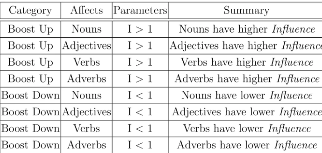
3.1 The 12 proximity measurements used as input into the genetic algo-rithm. . . 20 4.1 Parts of speech themed modifications. I is short forInfluence, where
the exact value for I is unique to each modification and determined through training. For the Boost Up category modifications, I is set to values greater than one and I is set to values less than one for the Boost Down category modifications. . . 41 4.2 Term to term themed modifications. I is short for Influence and is
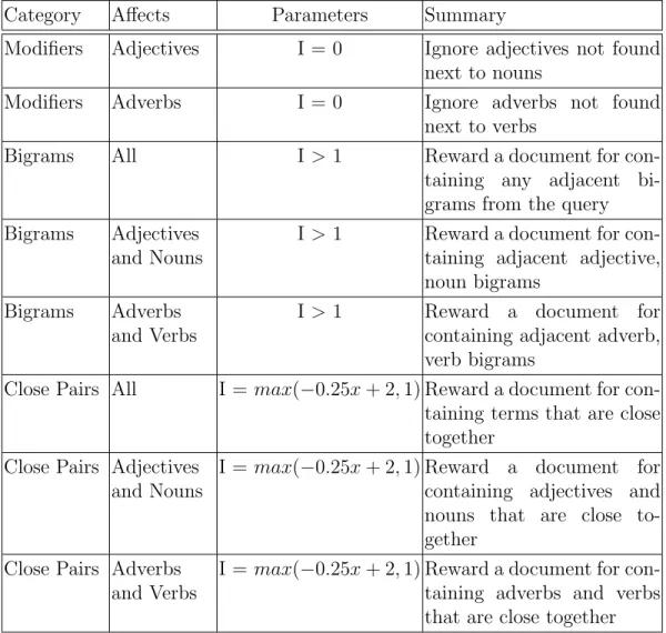
either a constant value or the result of a function. For the Modi-fiers category, I is set to zero because a term’s influence is ignored if the adjective/adverb is not found directly adjacent to its corre-sponding subject. For the Bigrams category, I is a unique, constant value greater than zero, which is determined through training. For the Close Pairs category, I is the result of a distance function that measures the separation between two query terms. . . 44 4.3 Term to document themed modifications. I is short forInfluenceand
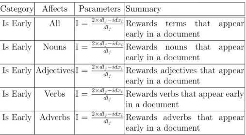
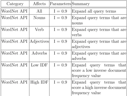
is set to a distance function that measures the distance between the start of a document and the current location of a term within that document. . . 45 4.4 WordNet API modifications for the query expansion theme. IDF is
short for Inverse Document Frequency. I is short for Influence. . . . 47 4.5 WordNet probability graph modifications for the query expansion
theme. RWSS is short for Random Walk Similarity Score. I is short for Influenceand takes on the value from the result of the Random Walk Similarity Score algorithm described in Section 4.3.4. . . 49 4.6 Word2Vec modifications for the query expansion theme. CSS is short
for Cosine Similarity Score. I is short forInfluenceand takes on the value resulting from Equation 2.6, applied to the Word2Vec vectors. 51 5.1 Document metadata for each benchmark. . . 55 5.2 Document parts of speech metadata for each benchmark. . . 55
5.3 Query metadata for each benchmark. . . 56 5.4 Query parts of speech metadata for each benchmark. . . 57 6.1 Expansion theme results. The values represent the percentage change
in mean average precision between Okapi BM25 and the modifica-tions for query expansions. . . 62 6.2 WordNet API query expansion data. . . 63 6.3 WordNet Graph query expansion data. Expansion terms were
cal-culated with a minimum similarity score of 0.02. . . 63 6.4 Word2Vec query expansion data. Expansion terms were calculated
with a minimum similarity score of 0.5. . . 64 6.5 Term - Document theme results. The values represent the
percent-age change in mean averpercent-age precision between Okapi BM25 and the modifications for the position of a term within a document. . . 65 6.6 Part of Speech theme results. The values represent the percentage
change in mean average precision between Okapi BM25 and the mod-ifications for a single term’s part of speech. . . 66 6.7 Term - Term theme results. The values represent the percentage
change in mean average precision between Okapi BM25 and the mod-ifications for the proximity between a pair of terms. . . 67 6.8 Expansion theme results. The values represent the percentage change
in mean average precision between Okapi BM25 and the modifica-tions for query expansions across multiple categories. WNG is short for WordNet Graph. WNA is short for WordNet API. W2V is short for Word2Vec. BIDF is short for Bottom Inverse Document Fre-quency. A colon (:) means that the category on the left hand side affects the part(s) of speech on the right hand side. . . 70 6.9 Term - Document theme results. The values represent the
percent-age change in mean averpercent-age precision between Okapi BM25 and the modifications for the position of a term within a document with re-spect to the start of a document across multiple parts of speech. . . 71
6.10 Part of Speech theme results. The values represent the percent-age change in mean averpercent-age precision between Okapi BM25 and the modifications for a single term’s part of speech across multiple cat-egories. ↑ symbolizes the Boost Up category, which contains mod-ifications with Influence values greater than one. ↓ symbolizes the Boost Down category, which contains modifications with Influence values less than one. . . 72 6.11 Term - Term theme results. The values represent the percentage
change in mean average precision between Okapi BM25 and the mod-ifications for the proximity between pairs of terms across multiple categories. CP is short for Close Proximity. B is short for Bigram. A colon (:) means that the category on the left hand side affects the part(s) of speech on the right hand side. . . 73 6.12 The change in mean average precision for modifications across
mul-tiple themes. QE is short for Query Expansion. TDA is short for Term - Document for Adjectives. TDNA is short for Term - Docu-ment for Nouns and Adjectives. TDVA is short for Term - DocuDocu-ment for Verbs and Adverbs. TT is short for Term - Term. POS is short for Parts of Speech. . . 76 6.13 The raw mean average precision (MAP) scores calculated against the
Lisa benchmark for the top scoring modification, the in-house built Okapi BM25 and cosine similarity models, and the out-of-the-box solutions for the Lucene and Solr search engines. . . 79 6.14 Percentage increases in performance when the top scoring
modifica-tion is compared to each of the other models. These percentages are calculated using the values presented in Table 6.13. . . 79
LIST OF FIGURES
Figure Page
2.1 The similarity between a query and document in the vector space model is computed as the cosine of the angle between the two vectors. 11 2.2 An example corpus containing three short documents. . . 13 2.3 An example inverted index derived from the corpus in Figure 2.2. . 13 2.4 Demonstrates how training samples are produced for the Word2Vec
neural network from a set of text with a window radius of two. . . . 18 3.1 High level algorithm for how LDA assigns topics and weights to words
in a corpus. . . 29 3.2 The CBOW architecture predicts the current word based on the
con-text, and the Skip-gram predicts surrounding words given the current word. . . 34 4.1 The stop words that were used in all the experiments. . . 36 4.2 A summary of the inverted index used in this thesis. The arrow
represents a mapping function. The angle brackets represent a single posting. The square brackets represent list notation. . . 38 4.3 JSON data structure format for accessing query expansion terms at
runtime. . . 46 6.1 Compares the precision and recall of Okapi BM25 and the top
Chapter 1 INTRODUCTION
Document retrieval systems are useful tools that allow users to obtain a set of doc-uments from a textual user query. In the field of information retrieval, a collection of documents is called a corpus. When people discuss information retrieval systems, most people think about Google’s search engine. At its core, Google’s search engine is much like a simple document retrieval system, except the corpus it is analyzing is the entire Internet. Their search engine works well because documents on the Internet are highly structured. For example, web pages are structured using HTML, which contain tags that provide context for the document. In addition to analyzing contex-tual information derived through HTML tags, Google’s search engine is able to return relevant web pages because it prioritizes “popular” web pages. Popularity is scored using their page rank algorithm, which is outside the scope of this introduction. How-ever, due to the technical nature of the page rank algorithm, Google’s search engine fails when users are trying to search for documents that are unpopular. This is a problem because documents can be both unpopular and relevant to the user’s search query. As a result, some documents are circularly discovered by many individuals and many other relevant and unpopular documents go undiscovered. This thesis focuses on improving document retrieval by developing methods to rank unstructured doc-uments based on their contents without relying on preexisting document structure, corpus context, or popularity scores.
It is important to research alternative ways to rank documents for a handful of reasons. First, systems that primarily rely on training data will not operate well if the domain of the training data is disjoint from the domain of the deployment envi-ronment. To generalize these models to many datasets, research has been conducted to try to minimize overfitting on training data [3, 38]. Ideally, the subject of training
data should be broad enough to cover all possible domains, however such an idealized set of data is difficult to gather. A system that heavily relies on training data will need to be retrained if the system is deployed in an environment which has a context that differs from the domain of the training data. Retraining or partially retraining a document retrieval system can take a significant period of time and also requires substantial effort from developers to collect and clean training data. On the other hand, an ad-hoc document retrieval model that does not require any training data can ideally be plugged into any corpus and operate effectively without any domain specific knowledge. This would save developers valuable time that can be spent on other pri-orities. A second reason to research alternative document ranking methods is that the structure of a corpus cannot always be assumed. As alluded to earlier in this chapter, Google’s page rank algorithm relies on structured content that exists in HTML web pages, such as hyper links, to grade the popularity of web domains. However, not all corpora contain structured content. Thus, the success of Google’s search engine is limited to corpora that contain these key contextual items. In a similar methodology to Google’s page rank algorithm, some researchers have experimented with clustering documents based on bibliographic citations located in a paper’s bibliography [42]. Graphing documents based on their citations is a useful way to analyze the differ-ences and similarities between documents, but this method is naturally limited to corpora that only contain documents with extensive bibliographic information. This is another example where the success of the document retrieval model is dependent on the specific structure of its documents. Ideally, researchers would like to develop a model that analyzes documents based just on their content and returns accurate results without having to rely on structured data or metadata. Such a model would perform efficiently on all corpora because the system’s performance would be agnostic to any preexisting structure. Third, it is often the case in a classroom or an industry setting where building a minimal viable product in a short amount of time is
impor-tant. In these time constrained environments, there simply isn’t enough time to train a sophisticated model, build a bibliographic similarity network, or insert structure into all documents inside a corpus. Instead, it might be better to use an ad-hoc document retrieval system that is guaranteed to operate efficiently and effectively on any corpus to speed up initial development and still maintaining high accuracy.
In addition to understanding the advantages of researching ad-hoc document retrieval methods, it is also important to understand why ranking documents based on their content is a difficult and unsolved problem. First, users are unpredictable. Users may have different expectations for the acceptable degree of relevance and or-dering for a list of documents for a particular search query. Second, there commonly exists a mismatch between the meaning of the user’s literal search query and the true meaning behind what the user intended to type. This mismatch between the user’s query and the user’s desire is known as the semantic gap. Closing the semantic gap is a fundamental area of research that directly affects how well a computer can differ-entiate between the user’s literal search query and the user’s desire. If closed, search engines would be able to return relevant documents with extremely high accuracy. Third, languages are dynamic with respect to time and location. This commonly oc-curs when a written language is shared across multiple cultures. For example, slang is extremely difficult to interpret because its meaning is dependent on the user’s culture. Text that reads, Eric likes chips, can be interpreted differently depending on the user’s culture. A user from America might had intended the statement to mean, Eric likes tortilla chips, whereas a user from Australia might had intended the statement to mean, Eric likes French fries because French fries are called chips in Australia. Fourth, as information grows at an exponential rate, search engines are expected to return relevant documents in a timely manner. So, data structures and algorithms must be built to perform efficiently. However, this becomes an issue for modern computers when there are many millions, or billions, of documents that need
to be quickly searched. In this case, system designers must decide if it is reasonable to search through every document in the corpus or a subset of documents.
As one might imagine, there are many more variables that can be considered when designing a document retrieval system. In addition to the above complexity, improving a document retrieval system is much like working with a black box. This is true because in real-world circumstances, the true relevance rating for a document, according to a search query, is not fully observable. Also, the many nuances of a language makes it difficult to design relevance criteria that can be applied to all corpora. As a result of these constraints, this thesis proposes hypotheses on corpus content and then designs and runs experiments to validate or to invalidate these hypotheses. If all experimental results pertaining to a particular hypothesis produce a better ordering of predefined relevant documents, then this will be seen as evidence that the hypothesis is correct.
This thesis will explore methods to improve a well known probabilistic doc-ument retrieval model called Okapi BM25 [36]. The overarching hypothesis is that the Okapi BM25 model is limited in quality of results because it is a bag of words approach to document retrieval. For example, the model does not take into account term proximity, query expansion, and term parts of speech. The model also lacks the ability to recognize semantically similar terms. For example, the word “smart” is treated completely differently than the word “intelligent. This thesis explores 42 different modifications to address the above issues. When the modifications are sys-tematically combined together, 87 unique variations of the Okapi BM25 model are produced. Each model is then validated against four difficult datasets and graded according to their mean average precision scores. The very best model from the vali-dation set is then tested against a separate, large dataset. The resulting model is able to outperform the original Okapi BM25 model in mean average precision by 10.25% and shows an increase in performance when evaluated over a precision recall curve.
The resulting model also outperforms two industry standard search engines, Lucene and Solr, by over 20% when compared using mean average precision.
The rest of this thesis is structured as follows. Chapter two provides back-ground on document retrieval models and relevant data structures. Chapter three explores related research on term proximity, semantic analysis, topic modeling, and language modeling. Chapter four provides implementation details for the various modifications to Okapi BM25. Chapter five discusses methods of validation, the rel-evant datasets, experimental protocols, and the results of the experiments. Lastly, chapter six gives concluding remarks and avenues for future research.
Chapter 2 BACKGROUND
Chapter 2 begins by briefly describing how Google’s search engine uses structured content and how the engine can fail. The section that follows describes unstructured search and why unstructured search is valuable. Then, the mathematical foundation for document retrieval systems will be presented. This theoretical section will describe the vector space model, the probabilistic model, and how documents are stored in information retrieval systems. Afterwards, the limitations of the vector space and probabilistic models are discussed by recognizing a semantic gap that exists between a user query and a set of documents. To help close the semantic gap, two open areas of research are introduced: WordNet and word embeddings.
2.1 Google Search
When the topic of search is brought up in conversation, many people will first think of Google’s search engine. But many are unaware of how it works and how it might fail. Google’s search engine organizes the web into a massive index using software programs called spiders [16]. Spiders take advantage of structured content inside HTML elements to make sense of the web pages. Spiders use hyper links to jump between web pages in order to discovered new web pages. The observable web is all the websites that are discovered by the spiders.
When a user submits a search query, Google’s search engine queries its enor-mous index and presents relevant links to the user [15]. The relevance for a web page is highly influenced by the number and weight of hyper links that point to a web page, as described in Google’s page rank algorithm [31].
Despite the successes of Google’s search engine, there exist situations where Google’s search engine fails. Due to the very nature of Google’s page rank algorithm,
Google gives priority to web documents that are visited frequently and are cited by popular websites. As a result, Google rarely orders documents with a small number of visits first, even if the content of the document is relevant to the query. This is a problem because unpopular documents can still contain credible and useful infor-mation. For example, a peer-reviewed paper published in a small conference which contains relevant information may never get returned first according to Google’s page rank algorithm. As a result of Google’s page rank algorithm, the documents which have the highest page rank are returned, which leads to a circular discovery of the same information.
2.2 Unstructured Search
An alternative way to process queries and documents is to rank documents without considering explicit inter and intra document structure. It is important to explore how search engines can rank documents using unstructured methods because not every corpus will contain structured content. In fact, there are many document collections that have very little structure. An example of an unstructured corpus is a collection of transcribed phone calls. If a user would like to search for conversations using the query, “couples discussing their family vacation plans,” a search engine would have to calculate the relevance of each document based on document and query text. These types of datasets are popular amongst speech recognition researchers and developers [45]. Another example of a document collection with no explicit structure is a set of research paper abstracts. Digital libraries, such as ACM and IEEE, have search engines that allow researchers to search papers based on a paper’s abstract. Hence, researching new methods to rank unstructured text has the possibility to enhance these search engines.
2.3 Document Retrieval Theory
A formalized mathematical understanding of document retrieval systems is now pre-sented in order to build the foundation for introducing the Okapi BM25 model and related works.
2.3.1 The Vector Space Model
The technical underpinnings of a document retrieval system can be formalized math-ematically [23]. Allow the set of distinct terms in a vocabulary to be denoted by V = {w1, w2, ...} and the corpus of documents to be denoted by D = {d1, d2, ...}.
Both documents and queries can be represented as vectors of length |V| and will contain a subset of unique terms from V. Each index in a vector is the count for a unique term in the document or query and each index represents the same term for all vectors with the same vocabulary. The equations for document and query vectors are shown here:
dj = (w1j, w2j, ..., w|V|j) (2.1) q = (w1, w2, ..., w|V|) (2.2)
wheredj is a document in the corpusDandwij is the count for a word indj. Likewise, q is a query and wi is the count for a word in q. When the ordering of words in a representation is ignored, the representation is called a bag of words. It is important to notice that document and query vectors are extremely sparse, meaning most of the elements inside a vector will be equal to zero. This is true because queries and documents will not contain a large proportion of the total vocabulary. For example, if the vocabulary contains 10,000 distinct terms and the text of a query is “yellow fluffy puppies,” then the vector representation of this query will contain three ones, each located at the corresponding index for “yellow,” “fluffy” and “puppy,” and 9,997 zeros in every other index location.
The size of the vocabulary can grow extremely large, so it is important to only store terms that have semantic meaning. It is very common for search engines to filter out “stop words,” which are terms that hold very little semantic meaning, such as {“a”, “of”, “is”, “the”}. In addition to filtering out stop words, many search engines will reduce terms down to their roots in order to further compress the vocabulary size, a process known as stemming. For example, “doggy” and “dogs” share the root “dog,” so any derivation of “dog” found in a document or vector will be recorded in the “dog” index. Filtering a corpus for stop words and stemming terms is very common in information retrieval experiments [41, 12, 49, 34, 48, 40].
The vector space model slightly modifies the vector representation of docu-ments and queries and uses a geometric distance function to compare the similarity of vectors. The vector space model recognizes the limitations of only accounting for the frequency of terms inside a document. For example, the term “dog” may appear frequently inside a dog-themed corpus. So, the word “dog” holds less meaning than other words found in the corpus. The vector space model fixes this issue by account-ing for how rare terms are with respect to all other terms inside the corpus. This property is known as the inverse document frequency of a term and is represented as the logarithmic quantity below:
idfi =log |D|
dfi
(2.3)
where idfi is the inverse document frequency for a term i, |D| is the number of documents in the corpus and dfi is the number of documents in the corpus that contain the term i. Notice that each term in a corpus is assigned an idf value that does not change unless the corpus changes.
The vector space model also takes into account the frequency of a term in a document. This is known as the term frequency and is represented as the quantity
below:
tfij =
fij
max{f1j,f2j, ...,f|V|j}
(2.4) where tfij is the term frequency for a term i and a document j. fij is the number of times a term i appears in documentj and max{f1j, f2j, ..., f|V|j} is the highest term
frequency in documentj. Notice that thetf value for a term changes with respect to the document.
The the weight for a term inside a document or query vector is the product between the term frequency and the inverse document frequency:
wij =tfij ∗idfi (2.5)
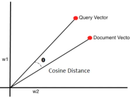
This tf-idf equation allows a query vector to be compared against document vectors with respect to a single corpus and a single vocabulary. Since documents and queries are represented as vectors, the similarity between two vectors can be computed by taking the cosine of the angle between the two vectors.
cosine(q, dj) =
< q•dj > ||q|| × ||dj||
(2.6)
The idea of the vector space model is that vectors that point in similar directions will be related to each other. When restricting values to the first quadrant (since documents and queries cannot have a negative number of terms), the cosine of the angle between two vectors gives a value from zero to one. A score that is close to zero indicates that two vectors are relevant because they point in similar directions. A score that is close to 1 indicates that two vectors are irrelevant because they point in different directions. Figure 2.1 shows a graphical representation of the cosine similarity metric.
Figure 2.1: The similarity between a query and document in the vector space model is computed as the cosine of the angle between the two vectors.
2.3.2 The Probabilistic Model
A well known information retrieval model is Okapi BM25 [36]. This model is rooted in statistics and assumes a bag of words interpretation for documents and queries. From statistics, the model assumes that an occurrence of a query term in a document is an independent event. These events happen in a specified interval, the start and end of a document. The probability that an event occurs is proportional to how rare a term is in a document collection (inverse document frequency). These criteria satisfy a Poisson distribution [17]. However, a Poisson distribution requires that the rate of occurrences for an event (terms in a document) is known ahead of time. This is problematic because there is no way of knowing the exact mean number of occurrences for a term in a given document ahead of time. Therefore, Okapi BM25 was built as an approximation of the Poisson distribution. The model’s equation bellow has been broken down into multiple components to help with the model’s overall explanation:
okapi(dj,q) =
X
ti∈q,dj
idfi ×tfij ×qtfi (2.7) Equation 2.7 gives a high level overview of the model’s ranking function. The model takes two inputs, a documentdj and a queryq and loops through each term ti that appears in both the document and the query. The score for a term is the product of three parts: the inverse document frequency (Equation 2.8), the term frequency
(Equation 2.9), and the query term frequency (Equation 2.10). The overall score for a pair of vectors is the sum of all the values. It is important to notice that the output value of the equation is unbounded, unlike the cosine metric used in the vector space model. Higher scores indicate that two vectors are similar to each other and lower scores indicate that two vectors are dissimilar to each other.
idfi = ln
|D| −dfi+ 0.5 dfi+ 0.5
(2.8) The first component of the model is the inverse document frequency. The idf for term ti (Equation 2.8) is a logarithmic function that gives a higher reward to terms that occur infrequently in the document collection. Similar to Equation 2.3 from the vector space model, idfi is a function of the number of documents in the corpus, |D|. tfij = (k1 +1)fij k1(1 −b+b dlj avdl) +fij (2.9) The second component of the model is the term frequency. The tf for a term ti in a document dj (Equation 2.9) is a linear function that gives a higher reward to terms that occur frequently in small documents. Term frequency punishes the document dj if the length of a document dlj is longer than the average document length avdl in the corpus. It is important to distinguish between longer and shorter documents because longer documents have more opportunities to contain query terms. b is a hyper parameter that adjusts how much a document is punished for its length andk1 is another hyper parameter that adjusts the weight of the term frequency with
respect to the entire model.
qtfi =
(k2 +1)fi k2+fi
d1 = “I heart APIs. You heart APIs”
d2 = “I use APIs at work”
d3 = “You work too much”
Figure 2.2: An example corpus containing three short documents.
I: [< d1,1>, < d2,1>] heart: [< d1,2>] APIs: [< d1,2>, < d2,1>]
You: [< d1,1>, < d2,1>] use: [< d2,1>] at: [< d2,1>]
work: [< d2,1>, < d3,1>] too: [< d3,1>] much: [< d3,1>]
Figure 2.3: An example inverted index derived from the corpus in Figure 2.2.
The third component of the model is the query term frequency. The qtf for a term ti (Equation 2.10) is a linear function that gives higher rewards for terms that appear multiple times in a query. fi is the frequency of a termti in a query q. k2 is a
hyper parameter that adjust the influence of the query term frequency with respect to the entire model.
2.3.3 The Inverted Index
An inverted index is an efficient data structure for digesting the information found within corpora by mapping each term in the vocabulary to a list of postings. A posting consists of a list of documents that contain the specified term and other relevant information, such as the term frequency. For example, examine the small corpus consisting of the three documents in Figure 2.2. The entries of the inverted index that would be produced from the three documents is shown in Figure 2.3. For each resulting entry in the inverted index, the key is the term on the left, the value is the list on the right, and a posting is represented as the values inside a pair of angle brackets. Within each posting, the first element is a reference to the document that contains the key term and the second element is the term frequency of the key term within the document. The inverted index is a helpful data structure in information retrieval systems because it abstracts away all the needed information found within a
corpus. After the contents of a corpus is transformed into entries in an inverted index, the corpus can usually be discarded from memory. Inverted indexes also dramatically increase the lookup time to obtain a set of documents that contain a particular word. Since the vector space model and the probabilistic model both rely on looking up documents that contain query terms, it makes sense why document retrieval systems utilize inverted indexes.
2.4 The Semantic Gap
One of the largest issues with the vector space and probabilistic retrieval models is their inability to cope with terms that are semantically similar and do not stem to the same root. For example, “smart” and “intelligent” are treated differently even though they have high semantic similarity. Often, users are more interested in the concepts that their queries represent rather than the exact phrasing of their queries. A document retrieval model that evaluates the query “smart animals” should be able to assign a high score to documents that contain the phrase “intelligent animals.” This limitation is known as the semantic gap. The research conducted in this thesis utilizes the following two tools to help close the semantic gap during experiments.
2.4.1 WordNet
To help close the semantic gap, researchers from Princeton University have attempted to organize the semantic relationships between English terms into cognitive synonyms in a project called WordNet [27]. A set of terms are considered to be cognitive synonyms, or synsets, of one another if the meanings of the terms are so similar to one another that they cannot be differentiated. From these synsets, conceptual, semantic, and lexical relations are built. The WordNet database can be used to extract valuable semantic information from terms, such as term definitions, various parts of speech, synonyms, hypernyms, hyponyms, and links to other related terms.
Words in the English language can have multiple definitions and uses so it is important to recognize these differences. A term inside WordNet subscribes to a set of synsets, where each synset has a different meaning. For example, the word “dog” belongs to eight different synsets. This is because dog can take on different meanings depending on the context of its usage. Some of the synsets that dog subscribes to are: a domestic dog of the Canis family, a smooth-textured sausage of minced beef or pork usually smoked, an informal way to refer to someone, etc. So determining the meaning of a word in a sentence is not as straightforward as looking up the definition of a term inside WordNet. There needs to be a way to determine the correct synset based on the term’s context. An area of research that aims to determine the correct usage of a term inside its context is called word sense disambiguation and a classic algorithm for determining the correct synset for a word is the Lesk Algorithm [22]. Given an ambiguous word and the context in which the word occurs, Lesk returns a synset with the highest number of overlapping words between: the various definitions from each synsets of each word in the context sentence and the different definitions from each synset of the ambiguous word. Once the appropriate synset is selected, semantically similar words can be chosen by selecting terms that subscribe to this synset. An in depth example of the Lesk algorithm ran on WordNet can be found in the footnote1.
Although WordNet shows that there exists a relationship between terms, such as “car” and “automobile,” WordNet does not provide the strength of the relationship between terms. Research has demonstrated that a graph can be extracted from the WordNet database to represent the sematic similarity between English terms [43]. In this graph, each node is represented by a term or phrase and each edge holds a weight that represents the probability that a user is interested in another term or phrase when given the current node. In this graph representation of WordNet, the
sum of probabilities from all the out edges is equal to one. The similarity between two terms is computed by performing a breadth-first traversal of the graph from each node in parallel to discover a path between the two nodes and then computing the product of the edges along this path [43]. In addition to computing the similarity between two known terms, semantically similar terms can be discovered for a given term by performing many random walks to discover neighboring nodes. A random walk is performed by randomly selecting an out edge, according to the probability distribution from the set of out edges, and traversing to the node pointed to by this edge. This process repeats itself for a given number of intervals defined as a hyper parameter. The nodes that are traversed most often represent the most semantically similar nodes.
Unfortunately, WordNet is difficult to maintain. As language evolves, the project demands continued effort in order to keep up with new additions and mod-ifications to the English language. As a result, WordNet does not have thorough entries for slang terms or figures of speech. For example, the phrase “down to Earth” is semantically similar to the words “practical” or “humble,” and this is not provided by WordNet. The best WordNet can do is analyze the above phrase through its parts, so “down to Earth” is interpreted as something that is literally close to the Earth’s surface.
2.4.2 Word Embeddings
Another method that can be used to help close the semantic gap is word embeddings. The core concept behind word embeddings is the Distributional Hypothesis [37]. The hypothesis states that words that appear in the same context share semantic meaning. In this model, each word in a vocabulary is represented as a vector and semantically similar words will have similar vectors. Just as how WordNet can be used to discover semantically similar terms, as can word embeddings. Semantically similar terms can
be discovered by looking up a word’s vector representation and then using a distance function, such as cosine similarity, to compute the distance between each word in the vocabulary.
Researchers have been experimenting with word embeddings since the early 2000s. One of the first papers to describe and implement a neural language model to produce word vectors was in [5]. The paper proposes a feed-forward neural network with a linear projection layer and a non-linear hidden layer to learn word vector representations and a neural probabilistic language model. This paper’s model took three weeks to train across 40 CPUs and produced perplexity scores that were 10% to 20% better than (at the time) state of the art smoothed trigram probabilistic language models.
Since the early 2000s, generating word embeddings has become much more efficient and accurate. In 2013, Google researchers published a technique called Word2Vec to learn high quality word vectors from huge data sets with billions of words and with millions of distinct vocabulary words [24]. Word2Vec is a semanti-cally driven method for representing terms that encode many linguistic regularities and patterns. The paper shows that word vectors could be built in less than a day using a shallow neural network and perform better than other industry standard lan-guage models. In a follow up paper by Google researchers [25], the researchers report that the word vectors produced using the Word2Vec method can represent syntactic analogies such as ”quick”:”quickly” and also semantic analogies, such as country to capital city relationships. This relationship can surprisingly be extracted using simple vector addition. For example,
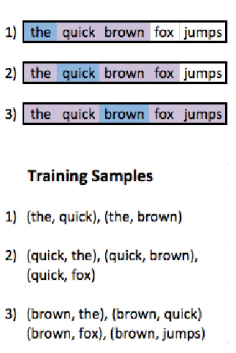
Figure 2.4: Demonstrates how training samples are produced for the Word2Vec neural network from a set of text with a window radius of two.
Word vectors allow for precise analogical reasoning and representation of the distributional context in which a word appears. To generate a word embedding using Google’s Word2Vec model, a shallow neural network is used to build feature vectors for each word in the vocabulary. These vectors encode the occurrence of prior and subsequent terms. Visually, prior and subsequent terms are encapsulated by a win-dow, where the size of the window is a hyper parameter. Shown in Figure 2.4, pairs of data points are drawn from the window of words in order to create the training samples for the neural network. For each training sample, the input to the neural network is the center window word and the expected output is a non center window word. Finally, the word vectors are extracted from the weights connecting the hidden layer and the output layer [18].
Chapter 3 RELATED WORKS
Chapter 3 explores related research on unstructured search. The first section will discuss previously established modifications to Okapi BM25 to increase the model’s accuracy. The next section will discuss other related techniques to analyze unstruc-tured text that do not utilize Okapi BM25.
3.1 Okapi BM25 Modifications
3.1.1 Genetic Programming
Ronan Cummins’ and Colm O’Riordan’s Learning in a Pairwise Term-Term Prox-imity Framework for Information Retrieval [12] uses a genetic algorithm to modify the Okapi BM25 model. This paper builds off their previous publication, where they propose a genetic algorithm to improve the vector space model [11]. The fitness func-tion for both papers rewards their system when an equafunc-tion modificafunc-tion results in an increase in the model’s mean average precision.
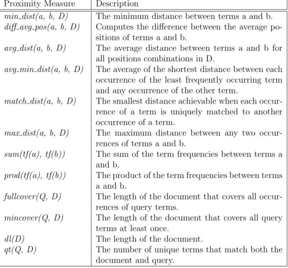
In order to derive a modified version of Okapi BM25, the researchers defines 12 different term proximity measures. These proximity measure were fed as input into their genetic algorithm. The algorithm then tried different combinations and weights for each proximity measure and output an equation that maximizes the mean average precision on a set of 69,500 documents and 55 queries. The best three func-tions produced using the genetic algorithm all resulted in equafunc-tions that used the minimum distance proximity measure and the average distance proximity measure. This suggests that the minimum distance and the average distance between query terms in a document is correlated to the relevance of a query and document. The proximity measures used in this experiment are defined in Table 3.1.1.
Proximity Measure Description
min dist(a, b, D) The minimum distance between terms a and b. diff avg pos(a, b, D) Computes the difference between the average
po-sitions of terms a and b.
avg dist(a, b, D) The average distance between terms a and b for all positions combinations in D.
avg min dist(a, b, D) The average of the shortest distance between each occurrence of the least frequently occurring term and any occurrence of the other term.
match dist(a, b, D) The smallest distance achievable when each occur-rence of a term is uniquely matched to another occurrence of a term.
max dist(a, b, D) The maximum distance between any two occur-rences of terms a and b.
sum(tf(a), tf(b)) The sum of the term frequencies between terms a and b.
prod(tf(a), tf(b)) The product of the term frequencies between terms a and b.
fullcover(Q, D) The length of the document that covers all occur-rences of query terms.
mincover(Q, D) The length of the document that covers all query terms at least once.
dl(D) The length of the document.
qt(Q, D) The number of unique terms that match both the document and query.
Table 3.1: The 12 proximity measurements used as input into the genetic algorithm.
3.1.2 Semantic Analysis
Bhatia’s and Kumar’s Contextual paradigm for ad hoc retrieval of user-centric web data [7] categorize the semantic relationship between pairs of terms in multi-term queries. The two categories that were defined in the paper were labeled “topic mod-ifying” and “topic collocating.” Topic modifying is where one query term represents a subject and the other query term modifies the subject. For example, “Indian Cur-rency” is a topic modifying query. On the other hand, topic collocating is where multiple query terms represent a single topic. For example, “data mining” is a topic
collocating query. The researchers propose three different hypotheses to test the properties of topic modifying and topic collocating queries:
1. Important terms always appear in the forefront of a document. 2. Related terms appear in close proximity to one another.
3. Important terms appear repeatedly in a document.
To test these hypotheses, an equation for each of the above hypotheses was derived. Then, 20 topic modifying and 10 topic collocating queries were typed into Google’s search engine to obtain the top 20 documents for each query. Each of the documents was then labeled as relevant or irrelevant by a human. The aforementioned equations were then used to reorder the returned documents and the precision was recorded at 5, 10, and 15 documents.
The results show that the reordering of topic modifying queries saw the largest increase in precision when ranking documents based on the smallest distance between query terms. This makes sense because a modifying term is most useful when found near its corresponding subject. Topic collocating queries saw the largest increase in precision when reordering documents based on their term frequencies and based on the smallest distance between query terms. These results make sense because the appearance of individual topic collocating terms do not have much semantic meaning if they are not found close together.
This thesis adopts the topic modifying and topic collocating principals laid out by Bhatia and Kumar. Unfortunately, the researchers do not provide a mech-anism for identifying topic modifying and topic collocating terms. As a result, this thesis assumes that topic modifying and topic collocating terms can be identified by evaluating the parts of speech of adjacent terms. In contrast to this research paper, this thesis explores how these techniques fair with long queries, as the queries used in this research paper were only two terms long. Lastly, this thesis takes inspiration
from Bhatia’s and Kumar’s first hypothesis, that important terms may appear at the front of a document.
3.1.3 Spans
A well researched area in term proximity is the idea of “spans.” A span is a segment of text from a document that incorporates all query terms, or a subset of the query terms. Spans have been shown to increase document retrieval accuracy for a number of cases. In Muhammad Rafique’s and Mehdi Hassan’s Utilizing Distinct Terms for Proximity and Phrases in the Document for Better Information Retrieval [34], the two researchers derive an equation that gives a greater reward if a large number of query terms appear close together in a document. The researchers’ implementation is unique because the system only accounts for the first occurrence of each query term. This modification allows the researchers to compress the system’s inverted index by only storing the location of the first occurrence of a term inside each posting. To validate their system, the researchers designed 25 custom queries and ran them the C50 dataset. The C50 dataset contains two repositories, one for testing and one for training, each containing 2,500 text files. Each text file is a passage written by a well known author and no information was provided on the custom queries. Their results show an increase in precision when observing the first five and ten returned documents by upwards to 20-30% and an increase to the mean average precision by around 15%, which is evidence that spans are a useful machanism for increasing the accuracy of document retrieval systems.
Researchers Ruihua Song, Ji-Rong Wen, and Wei-Ying Ma used spans to derive contextual information from queries in their paper, Viewing Term Proximity from a Different Perspective[41]. The paper introduces a technique to replace term frequency with an algorithm that incorporate term proximity using spans. Their algorithm splits a documents into non overlapping segments that contain one or more query terms
according to the rules of the algorithm. Intuitively, the relevance contribution is proportional to the density of each non-overlapping span. Mathematically, the score for an individual span is a function of the number of unique query terms divided by the width of the span, multiplied by two other hyper parameters. Thus, the total relevance contribution, rc, is the sum of scores from all the non-overlapping spans. The new term frequency formula for Okapi BM25 is as shown in Equation 3.1. Experiments were conducted on TREC (Text Retrieval Conference) disks 9, 10, and 11. Their results show an increase in precision when observing the first 5 and 10 returned documents by around 0.3% for disk 9, 10.4% for disk 10, and 4.4% for disk 11. tfij = (k1+ 1)rc k1(1−b+bavdldlj ) +rc (3.1) 3.1.4 Query Expansion
Query expansion is the process of reformulating a query to improve retrieval perfor-mance in information retrieval operations. The main motivation of query expansion is to include additional terms to express the original query in a more detailed way in order to increase the number of relevant documents identified [30]. As discussed in [30], there are three major areas of query expansion: query expansion using corpus dependent knowledge models, query expansion using relevance feedback, and query expansion using language models. Query expansion using corpus dependent knowl-edge models group similar words together in order to find suitable expansion terms. Query expansion using relevance feedback expands the query by extracting terms from either the first few returned documents or from known relevant document. Ex-tracting terms from the first few returned documents is not very effective for ad-hoc feedback systems because the first few returned documents are not guaranteed to be relevant to the query and will result in query drift [1]. Last, query expansion using
language models selects new terms according to the highest probability that the new term will appear in the context of the original query.
There are a number of researchers who have experimented with query expan-sion. Edward Fox’s research Lexical Relations: Enhancing Effectiveness of Informa-tion Retrieval Systems [14] explores a corpus dependent query expansion method. His algorithm builds unique lexical relations for document collections and shows how query expansion can affect the recall level of an information retrieval system. His main contribution is that the recall level of information retrieval systems can be im-proved if the knowledge model being used to expand the query is built from a corpus that shares the same lexical relations as the test corpus.
Research done by Olga Vechtomova, Stephen Robertson, and Susan Jones in their paper Query Expansion with Long Span Collocates [46] expounded on the idea of collocates1. The researchers aimed to identify all terms that significantly
co-occur with query terms within a specified window size. Their algorithm builds a list of possible expansion terms and weights these terms by their significance of association using statistical methods, such as Z-score. The researchers built two different knowledge models for query expansion. The first model was constructed from a global point of view, which included the entire corpus (a corpus dependent knowledge model) and the second model was built from a local point of view which contained a subset of the corpus that contained known relevant documents (a corpus dependent knowledge model with relevance feedback). To test their models, each query was ran using Okapi BM25 to gather average precision and recall scores. Then the query was expanded using one of the two models and was again run using Okapi BM25 to gather average precision and recall scores. Their results show that Okapi BM25 consistently performed worse when the query was expanded using the global
1Words which co-occur near each other with more than random probability are known as collo-cates
model. When using the local model, the average change in precision both improved and degraded for different sized queries. The researchers reason that their models fail to consistently and correctly expand queries because query terms have a very high level of dimensionality that can be derived from their contexts of occurrence.
A modern approach to query expansion uses language models. Language mod-els take advantage of the high levmod-els of the contextual dimensionality that a term can exhibit within a document (language models are explored in detail in Section 3.3). Some researchers, such as Saar Kuzi, Anna Shtok, and Oren Kurland, in their paper Query Expansion Using Word Embeddings [19] have successfully been able to expand queries and increase mean average precision using language models trained on the same corpus that their document retrieval system is analyzing. Since training lan-guage models from scratch require a lot of training data, their models were trained on large TREC (Text Retrieval Conference) disks, which were also the same datasets that their document retrieval system was analyzing. This type of local training is consistent with the preceding corpus dependent models as it appears that query ex-pansion is best conducted when a lexicon is built from the same domain as the target corpus.
Despite some of the successes of the above researchers, other researchers doubt the potential of query expansion for ad-hoc retrieval. Anton Bakhtin, Yury Usti-novskiy, and Pavel Serdyukov in their workPredicting the Impact of Expansion Terms Using Semantic and User Interaction Features [2] suggest that query expansion does not improve query performance. The researchers examine query expansion via corpus dependent knowledge models and claim that query expansions will more than likely hurt the system’s recall due to vocabulary mismatch, or hurt the system’s precision due to topic drift. The researchers sampled 35,000 unique queries from a Yandex search engine query log and computed the difference between the F-score, precision, and recall for documents being retrieved from a query without any expansions and
from a query with expansions. The results of their experiments show that in around 84% of cases, query expansion does not change the query’s overall performance, which may imply that query expansions are not a very efficient mechanism for improving ad-hoc document retrieval systems.
3.1.5 BM25F
Some researchers have proposed an extension of the Okapi BM25 model that assumes that some parts of a document are more relevant to the query than other parts of a document. This idea was first developed for web search and takes advantage of explicit structure inside HTML tags and RDF triples. RDF is a Semantic Web technology which stands for Resource Description Framework that was developed to give semantic meaning to elements on web pages [26]. Metadata in the RDF model is expressed as triples: subject, predicate, and object, which are encoded as URI’s. For example, a web page on the movie Deadpool can contain a hyperlink to the movie’s director, Tim Miller, which indicates that Deadpool was directed by Tim Miller. This information can be expressed explicitly as a RDF triple: (Deadpool, directed by, Tim Miller), where the movie Deadpool is the subject, directed by is the predicate, and Tim Miller is the object. RDF triples allow humans to encode documents with semantic meaning which computers can then use to better understand the content of documents.
Researchers first took advantage of HTML tags and RDF triples to create the BM25F probabilistic retrieval model [33]. BM25F is similar to Okapi BM25 with the addition that for each term, a weight variable is used to either scale up or scale down the relevance of the term depending on the context in which the term is discovered. The weight variable is heuristically set. For example, terms discovered in a HTML title element or a RDF triple subject may be given a positive boost to the term’s score if these fields appear to be relevant to the query. Experiments have shown that
using BM25F can improve the Okapi BM25 model when evaluated over precision and mean average precision. The downside to the model is that BM25F requires that documents be structured with HTML and/or RDF triples.
With the growing popularity and success of BM25F, some researchers set out to apply similar techniques to unstructured text. For example, Roi Blanco and Paolo Boldi in their paperExtending BM25 with Multiple Query Operators [8] built a model to generalize BM25F to unstructured text. The basic idea of their approach is that a document is split into “virtual regions.” Much like Okapi BM25F, each region rep-resents a different level of relevance to the query and will be weighted proportionally to its statistical significance. These virtual regions are generated similar to the span examples in Section 3.1.3, where a high density of query terms in a subsection of a document may indicate greater importance than a less dense area of a document. In a two pass procedure, Blanco’s and Boldi’s algorithm first partitions a document and assigns weight values to each partition. Then, the document is scored in the same way as BM25F. Their algorithm was tested against five large document collections containing around 95 million documents and they report a consistent increase in mean average precision over both Okapi BM25 and BM25F.
3.2 Topic Models
Topic models attempt to understand the semantic structure of text by assuming that there is some hidden structure in a document that can be discovered and exploit it in order to cluster similar documents.
3.2.1 Latent Semantic Indexing
Latent Semantic Indexing (LSI) is an early topic model that uses singular-value de-composition in order to expose semantic relationships between documents in a corpus [39]. Singular-value decomposition is a mathematical procedure that attempts to
re-duce the rank of a matrix by approximating the matrix’s row (or column) vectors by a smaller set of linearly independent vectors (vectors are linearly independent of each other if two vectors are not scalar multiples of each other or a linear combination of other vectors in the set) [28]. In LSI, the matrix that is to be approximated is the corpus, where each row is a document and each column is a term in the vocabulary.
In an early paper that presents the LSI algorithm [39], the researchers pro-posed that a document-term matrix can be approximated by a set of 100 linearly independent features that can be linearly combined to approximate each document in the corpus. Each document in the corpus can then be plotted in hyperspace ac-cording to the document’s linear approximation formula. A document’s position in space serves as a document’s identity and neighboring documents in this space should have similar topics. Similarly, a query can be analyzed as a weighted combination of terms and be plotted in the same hyperspace. From here, LSI borrows from the vector space model by computing the angle between the query point and the surrounding document points to compute similarity scores.
LSI takes into account the semantic similarities between words by nature of its design because a query with terms that do not appear in a document may still end up close to a document in hyperspace. As a result, a query can return documents with terms that are semantically similar to query terms. However, LSI falls short because it does not take into account words that have multiple definitions. For example, the term “bark” can be used in two different contexts, “the dog barks” and “tree bark.” Therefore, a document discussing how a dog barks and another document discussing tree bark may appear close to each other in hyperspace. Since so many words have multiple use cases, it makes sense to extend LSI to better accommodate words that relate to multiple topics, or a set of high level ideas such as sports, music, education, etc.
foreach document d∈D do foreach word w∈d do
foreach topic t do
p1 = Proportion of words in d currently assigned to t;
p2 = Proportion of assignments to t over all documents from w; p3 = p1 *p2;
w←(t,p3); end
end end
Figure 3.1: High level algorithm for how LDA assigns topics and weights to words in a corpus.
3.2.2 Latent Dirichlet Allocation
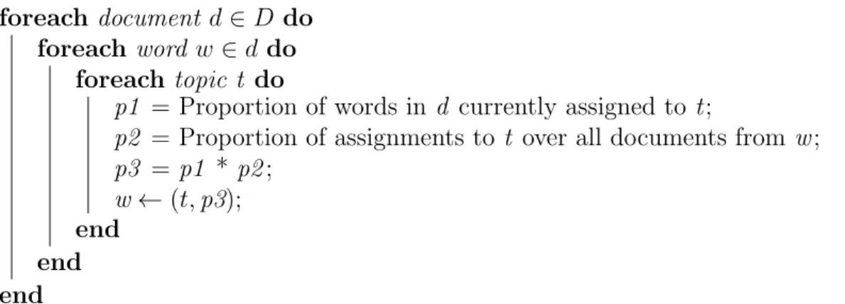
Latent Dirichlet Allocation (LDA) is similar to LSI, but it is more robust to word ambiguity [13]. LDA is more powerful than LSI because each word in the vocabulary can be expressed by a set of topics with a corresponding set of weights. For example, the term “bark” can be expressed by a mixture of topics such as “dog” and “tree.” The word “bark” can also relate to “dog” and “tree” in different proportions, such as 60% “dog” and 40% “tree.” These proportions will depend on the subject domain of the corpus. In LDA, a document is a combination of words, where each word belongs to a combination of topics. So a document can also be expressed as a combination of topics and weights, much like a recipe. For example, a document may be 35% sports, 45% music, and 20% education. These topic proportions can then be used to compare queries and documents. For LDA, queries and documents are relevant to one another if they are composed of a similar combination of topics.
LDA must be trained using a corpus in order to determine the best com-bination of topics and weights for a particular term. Initially, words are assigned randomly to topics. Then, for each word in every document and every topic, a word is reassigned to a topic according to the probability that a topic generates that word. A rough overview of the pseudocode can be found in Figure 3.1. The disadvantage
to LDA is that the number of topics is chosen as a hyper parameter that must be empirically determined. Another disadvantage is that LDA does not take into ac-count the proximity and ordering of terms inside a document because it is a bag of words model. Dispite these disadvantages, LDA is still an effective tool for clustering documents. The next section will explore language models, which emphasize term proximities in order to extract a term’s semantic meaning.
3.3 Language Models
A language model can be used to derive semantic meaning from terms using term proximity. Language models represent the semantic meaning of terms as a probabil-ity distribution that represents the likelihood that a term can be found near other terms. This term probability distribution can then be used to predict the likelihood that a term may appear near a set of different terms. As a result, language models lend themselves well to solve problems in fields beyond document retrieval, such as speech recognition [47, 45]. A common problem in speech to text programs is that a sound recording can be represented in many different ways, most of which make no grammatical sense. For example, the phrases “I saw a van” and “eyes awe of an” are acoustically similar to one another, but “I saw a van” would be a more likely tran-scription of the audio file because there is a higher probability that these terms would appear in each other’s contexts. Language models solve this problem by calculating the probability that a term will appear in a particular context rather than simply returning terms based on their acoustics. This behavior is exploited by document re-trieval engines to both derive query expansion terms that make sense according to the term’s context and to directly score the similarity between documents and queries.
3.3.1 The Probabilistic Language Model
A probabilistic language model can be used to score the relevance between a document and a query by computing the probability that a document will generate a query [20]. To perform this calculation, a probability distribution is first built for each document. In unigram language models, terms are treated as independent events. Hence, the probability that a word appears in a document is given as the conditional probability between the word and the document [23], as shown in Equation 3.2,
P(wij|dj) = fij
|dj| (3.2)
where fij is the frequency of term i in document j and |dj| is the total number of words in documentj. Therefore, the probability that a document generates the terms in a query, q = (w1, w2, ..., wm), of length m is the product of all the probabilities that each query term appears in the document [20], as shown in Equation 3.3.
P(qi|dj) = m
Y
i=1
P(wij|dj) (3.3)
A unigram language model can be expanded to account for a term’s context in order to gain more insight into a term’s semantic meaning. To do so, the probability of a term will be modified to depend on previous terms in its context, as given by Equation 3.4,
P(wn) = P(wn|w1, w2, ..., wn−1) (3.4)
where P(A, B, C) is expanded to P(A)P(B|A)P(C|A, B) and n is the nth term in a document. As one might suggest, accounting for all the preceding terms over complicates the language model. In order to simplify training and to reduce the combination of terms that can appear in another term’s context, the probability of a term can be simplified to only depend on a few preceding terms. The number of
preceding terms will be indicated by the variable k. This is known as the Markov Assumption [10]. Using the Markov Assumption, the probability of a term in a document reduces to Equation 3.5.
P(wn) = P(wn|wn−k..., wn−1) (3.5)
When k = 1, orP(wn) = P(wn|wn−1), the system is called a bigram language model.
When k = 2, or P(wn) = P(wn|wn−2, wn−1) the system is called a trigram language
model. The probability that a term appears in a document for small values of k now depends on the frequency of phrases that appear before a term and including that term. The probability that a term appears in a document for a bigram model is shown in Equation 3.6,
P(wi|wi−1)j =
count(wi−1, wi)j count(wi−1)j
(3.6)
wherecount(wi−1, wi)j is the number of times the 2-tuple (wi−1, wi) appears in docu-mentj and count(wi−1)j is the number of times the word wi−1 appears in document
j. For example, if a document contains the text “My dog makes him happy and her happy” thenP(“and”|“happy”) = countcount(“happy and(“happy”)”) = 12
Language models compute the similarity between a query and a document by determining the probability that a document’s probability distribution generates a query. For example, the probability that a query qi = (w1, w2, ..., wm) is generated from a document in a bigram language model is the product of each conditional probability for each pair of terms, as shown in Equation 3.7.
In Equation 3.7,sand s0 are special symbols reserved for the start and end of queries and document. Whenk is generalized to any number, the model is called an N-gram language model.
The N-gram language model has a few disadvantages. The number of different possible phrases grows exponentially with respect to the vocabulary size, especially whenkis large. Also, it is not likely that a training set will contain every combination of phrases for high values of k. Thus, the discrete probability distribution that is created most likely has missing values and it is not clear what exactly to do when a query contains a word that is not contained in a document. This is a problem because missing words will result in zero valued probabilities. To fix this problem, language models are usually smoothed to mimic continuous distributions. The main purpose of smoothing is to assign a non-zero probability to unseen words and phrases. One of the simplest smoothing techniques is called Laplace smoothing [50], where an extra count is added to each term. Another popular way to smooth a language model is by using linear interpolation with a background collection model, or by using word sense information from semantic databases (such as WordNet) [21]. Many more techniques are outlined in [50].
3.3.2 Neural Language Models
The absence of a continuous distribution in the probabilistic language model motivates a language model that utilizes neural networks. By the nature of their design, neural networks lend themselves well to generating continuous distributions because the training process will adjust the weights and biases for groups of neurons. Similar to a statistical language model, a neural language model computes the similarity score between a document and a query as the probability that a query is generated by a document. Neural language models are used to generate the high quality Word2Vec word embeddings as described in Section 2.4.2. Unlike statistical language models,
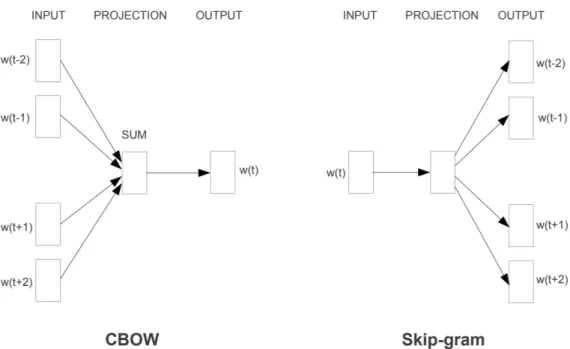
Figure 3.2: The CBOW architecture predicts the current word based on the context, and the Skip-gram predicts surrounding words given the cur-rent word.
neural language models are trained using both previous and subsequent terms. In the case of Word2Vec, two interesting architectures are derived. The Continuous Bag-of-Words (CBOW) model is able to predict a term according to the terms in the current term’s context [24]. This behavior is similar to that of the behavior for probabilistic language models. The other Word2Vec architecture is the Continuous Skip-gram model, which tries to classify a word based on another word in the sentence [24]. More precisely, this model is used to predict words within a certain range before and after the current word. The Skip-gram model can hypothetically be used for query expansion because it allows search engines to recognize terms that are likely to appear to each other’s contexts. For example, the term “Hong” is commonly found right before the term “Kong.” So if a user leaves out “Kong” when searching for the country Hong Kong, the Skip-gram model can be used to infer the user’s intension. Figure 3.2 provides a visual summary of the CBOW and Skip-gram models.