Outlier Detection for Mixed Model with Application to RNA-Seq Data

Application to RNA-Seq Data

by Tzu-Ying Liu

A dissertation submitted in partial fulfillment of the requirements for the degree of

Doctor of Philosophy (Biostatistics)

in The University of Michigan 2018

Doctoral Committee:

Associate Professor Hui Jiang, Chair Professor Jack Kalbfleisch

Associate Professor Srijan Sen Professor Peter X.K. Song Professor Ji Zhu

[email protected]

ORCID iD: 0000-0001-7533-4134 c

I would like to thank my program advisor, Professor Hui Jiang and my committee members, Professor Srijan Sen of the Department of Psychiatry and Molecular and Behavioral Neuroscience Institute, Professor Ji Zhu of the Department of Statistics, Professor Peter Song and Professor Jack Kalbfleisch of Department of Biostatistics, for their exceedingly insightful comments that improved my research.

I also would like to express my gratitude to the two anonymous reviewers and the associate editor of The Journal of Computational and Graphical Statistics for their suggestions on my first project, especially for the image restoration application and the extension to high-dimension settings. I am very grateful to our collaborators, Dr. Marcin Cieslik, and Professor Arul Chinnaiyan; they provided me with helpful suggestions and encouragement. Finally, I would like to thank the funding investiga-tor, Professor Alex Tsodikov. The research was supported by NIH Prostate SPORE grant 5P50CA186786.

ACKNOWLEDGEMENTS . . . i

LIST OF FIGURES . . . iv

LIST OF TABLES . . . vii

ABSTRACT. . . viii

CHAPTER I. Introduction . . . 1

II. Minimizing Sum of Truncated Convex Functions . . . 4

2.1 Introduction . . . 4

2.2 Applications . . . 6

2.2.1 Outlier detection in linear models . . . 6

2.2.2 Convex shape placement . . . 9

2.2.3 Signal and image restoration . . . 10

2.3 Methods . . . 11

2.3.1 Notations . . . 12

2.3.2 The general algorithm . . . 13

2.3.3 Implementation in low-dimensional settings . . . 14

2.3.4 Extension to high-dimensional settings . . . 16

2.3.5 Time complexity analysis . . . 17

2.4 Experiments . . . 19

2.4.1 Outlier detection in simple linear regression . . . 19

2.4.2 Sum of truncated quadratic functions . . . 20

2.4.3 Convex shape placement . . . 23

2.4.4 Signal and image restoration . . . 23

2.5 Discussion . . . 27

III. Integrating Poly(A) Capture and Exome Capture RNA-Seq Data . . . . 29

3.1 Introduction . . . 29

3.2 The Data . . . 33

3.3 Evidence of differences between the two types of measurements . . . 35

3.4 Converting capture sequencing measurements to Poly(A) measurements . . . 37

3.4.1 Notation . . . 39

3.4.2 Comparing prediction by genewise simple regression and mixed effect model . . . 39

3.5 Results . . . 40

3.6 Discussion . . . 43

IV. Outlier Detection for Mixed Model. . . 47

4.1 Extending mixed effect model for detecting individual outliers and outlying random effects . . . 47

4.2 Estimation Scheme . . . 49

4.3 Estimate the outliers and predict the random effects by Penalized Maximum Likelihood Estimation . . . 51

4.3.1 Separation of the objective function by incorporating the predictors of the random effects . . . 53

4.3.2 Transform the objective function into a sum of truncated quadratic functions . . . 55

4.3.3 Summary of estimating ∆ andδ. . . 59

4.4 DetermineλO andλG . . . 60

4.4.1 Variance of the conditional residuals and predicted random effects 61 4.4.2 Determine the cutoffs for conditional residuals and predicted ran-dom effects . . . 62

4.5 Dilation factor . . . 65

4.6 Simulation Study . . . 67

4.7 Application to RNA-Seq data . . . 70

4.8 Discussion . . . 73

V. Discussion. . . 75

APPENDIX. . . 77

A1 Appendix for Chapter II . . . 77

A1.1 Application on detecting differential gene expression with`0-penalized models . . . 77

A1.2 Algorithms described in Section 2.3 . . . 79

A1.3 The Θ-IPOD algorithm for robust linear regression . . . 81

A1.4 The difference of convex (DC) functions algorithm . . . 81

A1.5 The iterative marginal optimization (IMO) algorithm for signal and image restoration . . . 82

A1.6 Proofs . . . 83

A1.7 Supplementary figures and tables . . . 87

BIBLIOGRAPHY. . . 90

Figure

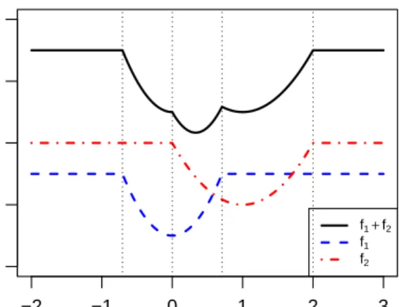
2.1 The sum of two truncated quadratic functions f1+f2 (in black), where f1(x) =

min{4x2_{+ 1,3} (in blue) andf}

2(x) = min{2(x−1)2+ 2,4}(in red). . . 6

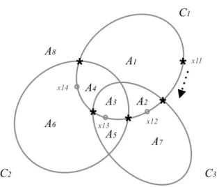
2.2 The corresponding Ci’s of three convex functions f1, f2, f3 define on R2, where

Ci ={x :fi(x)≤0}. The boundaries of {Ci}3i=1 partition R

2 _{into eight disjoint}

pieces {Aj}8

j=1. . . 13

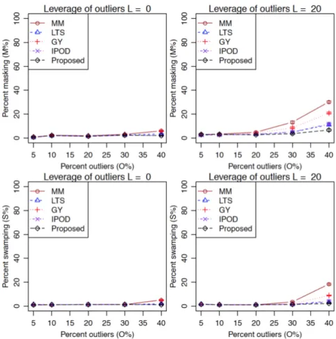
2.3 Comparison of different methods for outlier detection in simple linear regression. The figures show the mean percents of masking (top) and swamping (bottom) for different leverages of outliers: L= 0 (left) andL= 20 (right) and different percents of outliers (O%) for all the methods using 100 simulated replicates. The standard errors of the means are shown as error bars. When estimating the regression coef-ficients and identifying the outliers, we assume that the σ2 _{is known and is 1. In}

other words, we estimate only β and γ in (2.2). When implementing MM, LTS and GY estimators, the fact thatσ2_{is known is not exploited because we use}

pack-aged functions for these methods, which assume σ2 _{to be unknown and have no}

arguments for specifyingσ2_{. . . . . 21}

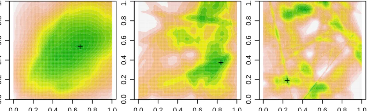
2.4 Contour plots of randomly generated sum of truncated quadratic functions inR2_.

Global minima are marked with the plus sign. . . 23 2.5 Comparison of different algorithms for minimizing the sum of 50 randomly

gen-erated truncated quardratic funstions in 2-D. The figure shows the mean success rates (in percents) for all the methods using 100 simulated replicates for different complexities of the functions (C). The standard errors of the means are shown as error bars. . . 24 2.6 Simulated random signal (left) and restored signal (right) are shown in solid lines.

The underlying true signal are shown in dashed lines. . . 25 2.7 Restoration of synthetic and real images. For each row, from left to right: original

image, image with Gaussian noise added, image restored using Gaussian smoothing with a 5×5 kernel and image restored using proposed algorithm. . . 27 3.1 mRNA isolation, adopted from [21]. In the process of RNA-seq library preparation,

RNAs are first isolated from tissue samples using commercial kits. Then mRNAs are isolated from total RNAs by annealing to oligo-dT beads. rRNAs and tRNAs are washed away before mRNAs are released from the beads. . . 31 3.2 RNA-seq workflow, adopted from [27]. The purified mRNAs are first fragmented

into smaller pieces and reverse-transcribed to complementary DNAs (cDNAs). Af-ter formation of one strand of cDNA, the mRNA strand is removed and replaced by another strand of cDNA to generate a double-stranded cDNAs. Each end of the double-stranded DNA is then repaired, adenylated and ligated by adaptor before being enriched by polymerase chain reaction (PCR). Once a library has passed the quality control, it can be sent to various sequencing platforms and generate read counts data. . . 32

tureSeq libraries had a difference from the poly(A) measurements as -2.7, -1.5, -1.1, -0.6, 0.1, and 0.7. The RINs range from 2.5 from 10 with a mean of 8.6 and a median of 9.2. The 1st and the 3rd quartiles are 8.1 and 9.6. . . 34 3.4 Cluster analysis on the paired CaptureSeq and Poly(A) log2(CPM) measurements

from 25 prostate cancer patients. Each row represent a gene and each column represent either a library of CaptureSeq ( columns with purple tags on the top) or Poly(A) (columns with orange tags on the top) measurements. The genes are the top 50 most varied genes across the 50 libraries. We used the Euclidean distance and the complete method of Hierarchical clustering on the genes. . . 36 3.5 Box plots of the number of significant genes in each experiment comparing two

groups of randomly drawn subjects . . . 38 3.6 Prediction by the mixed model and genewise fixed effect models on libraries with

RIN≥7: correlation of predicted and actual poly(A) log2-CPMs across all genes and all samples, based on 30 replicates for each sample size. . . 41 3.7 Prediction by the mixed model and genewise fixed effect models on libraries with

RIN≥7: RMSE of predicted and actual poly(A) log2-CPMs across all genes and all samples, based on 30 replicates for each sample size. . . 41 3.8 Cluster analysis on the paired predicted Poly(A) measurements based on

cap-ture sequencing measurements and true Poly(A) log2(CPM) measurements from 25 prostate cancer patients. Each row represents a gene, and each column rep-resent either a predicted Poly(A) library ( columns with purple tags on the top) or true Poly(A) (columns with orange tags on the top) measurements. The genes are the top 50 most varied genes across the 50 libraries. We used the Euclidean distance and the complete method of Hierarchical clustering on the genes. The clustering is now by subject, which is suggested by the neighboring of same subject identification numbers. . . 42 3.9 Distribution of the gene-wise ordinary least squares (OLS) estimates by having

the paired the Exome Capture RNA-Seq measurements regressed on the Poly(A) Capture RNA-Seq measurements. The arrows indicate identified causes for some of the gene-specific random effects to be outliers of the assumed bivariate normal distribution. . . 44 3.10 Examples of genes whose OLS estimates lie in the right lower quadrant of in

Fig-ure 3.9. The smaller clusters of observations shared the same sample identifiers across multiple genes, which suggests the existence of batch effects. . . 44 3.11 The distribution of and the correlations between the total length of exons in a

gene, the proportion of the bases in the exons that are either ”G” or ”C”, and the proportion of the length that is covered by the first generation probes of CaptureSeq designed by our collaborative biotech company, the intercepts, the slopes and the residual standard error of the genewise simple regressions by regressing Poly(A) log2(CPM) measurements on CaptureSeq log2(CPM) measurements. . . 45 3.12 Distributions of the Exome Capture RNA-Seq and the Poly(A) Capture RNA-Seq

measurements. The first row shows the distribution of mean log2 count per million (CPM) for each gene. The second row displays the inverse relationship between the variance of log2CPM and the mean raw count. The third row illustrates the libraries sizes for all samples, which are measured by both Exome Capture and Poly(A) Capture methods. . . 46 4.1 Estimation scheme of the proposed method. . . 51

for 18,000 genes from 100 subjects. We use a mixed model to the predict Poly(A) measurements based on a single predictor, the Capture RNA-Seq measurements with gene-specific random intercepts and slopes. Because the outlying gene-specific effects will be estimated as zeros in the proposed method, we use estimated coef-ficients from the simple regression in to demonstrate the relative positions of the detected outlying random effects (red) and normal random effects (black). . . 70 4.3 The scatter plot of Capture and Poly(A) RNA-Seq measurements from one of the

undetected outlying genes whose OLS estimates lies in the right upper quadrant in Figure 4.2. The gene-specific OLS estimates the standard error to be 1.1 while the common standard error assumed by the proposed method across all genes is 0.46. There are also unequal variances among observations within a gene. . . 71 4.4 The scatter plot of Capture and Poly(A) RNA-Seq measurements from one of the

undetected outlying genes whose OLS estimates lies in the left upper quadrant in Figure 4.2. The gene-specific OLS estimates the standard error to be 0.72 while the common standard error assumed by the proposed method across all genes is 0.46. There are also unequal variances among observations within a gene. . . 72 4.5 The scatter plot of Capture and Poly(A) RNA-Seq measurements from one of

the detected genes whose OLS estimates are not outlying. The gene-specific OLS estimates the standard error to be 1.9 while the common standard error assumed by the proposed method across all genes is 0.46. There are also unequal variances among observations within a gene. . . 72 A1 Placement of different convex shapes to cover the maximum number of points

uni-formly sampled from the unit square. . . 87 A2 Restoration of images. For each row, from left to right: original image, image with

Gaussian noise added, image restored using Gaussian smoothing with a 5×5 kernel and image restored using proposed algorithm. . . 87

Table

2.1 Comparison of different algorithms for signal restoration. The table shows the mean success rates (in percents), relative losses, root mean square errors (RMSE), as well as running times (in seconds) for all the methods using 100 simulated replicates. The standard errors of the means are given in parentheses. . . 26 3.1 Origins of cancer tissues of the 372 patients. . . 33 3.2 Nonzero coefficients of the penalized regression for classifying samples

from the two technologies. We tuned the Elastic Net regression model using a sequence ofα(from 0 to 1, with a step of 0.1), which determined the proportion of quadratic and L1 norm in the penalty term, and 10-fold cross-validation to choose λ. We trained the model on 272 pairs of measurements and then tested the model on the other 100 pairs. The misclassification rate on the test set is 0.005.

. . . 37 3.3 Differential expression experiments of randomly drawn subjects.

Num-ber of genes found to be significantly differentially expressed for more than 50 times in a total of 1000 experiments. . . 37 4.1 Summary of the estimates with corresponding outlyingness . . . 60 4.2 Outlier detection for small data sets composed of 20 genes, each with10 paired

measurements. The results are based on the medians of the 100 replicates. For the proposed method, the ideal masking (false negative) rate is 0 and the swamping (false positive) rate should be close to the user-defined thresholdα, which is 5% in the simulation setting. . . 68 4.3 Outlier detection for data sets composed of 2000 genes, each with10 paired

mea-surements. The results are based on the medians of the 100 replicates. For the proposed method, the ideal masking (false negative) rate is 0 and the swamping (false positive) rate should be close to the user-defined thresholdα, which is 5% in the simulation setting. . . 69 4.4 Parameter estimation by the naive method and the proposed method based on

data sets composed of 20 genes, each with 10 paired measurements. The results are based on the medians of the 100 replicates. . . 69 4.5 Parameter estimation by the naive method and the proposed method based data

sets composed of 2000 genes, each with 10 paired measurements. The results are based on the medians of the 100 replicates. . . 69 A1 Comparison of different methods for outlier detection in simple linear regression.

The table shows the leverages of outliers (L), percents of outliers (O%) and mean percents of masking and swamping for all the methods using 100 simulated repli-cates. The standard errors of the means are given in parentheses. . . 88 A2 Stopping criteria of the simulation studies in Sections 2.4.2 and 2.4.4 . . . 88 A3 Comparison of different algorithms for global optimization of the sum of 50

ran-domly generated truncated quadratic functions in 2-D. The table shows the com-plexities of the functions (C) as well as mean success rates (in percents) and running times (in seconds) for all the methods using 100 simulated replicates. The standard errors of the means are given in parentheses. . . 89

Extracting messenger RNA (mRNA) molecules using oligo-dT probes targeting on the Poly(A) tail is common in RNA-sequencing (RNA-seq) experiments. This approach, however, is limited when the specimen is profoundly degraded or formalin-fixed such that either the majority of mRNAs have lost their Poly(A) tails or the oligo-dT probes do not anneal with the formalin-altered adenines. For this prob-lem, a new protocol called capture RNA sequencing was developed using probes for target sequences, which gives unbiased estimates of RNA abundance even when the specimens are degraded. However, despite the effectiveness of capture sequencing, mRNA purification by the traditional Poly(A) protocol still underlies most refer-ence libraries. A bridging mechanism that makes the two types of measurements comparable is needed for data integration and efficient use of information.

In the first project, we developed an optimization algorithm that was later applied to outlier detection in a linear mixed model for data integration. In particular, we minimized the sum of truncated convex functions, which is often encountered in mod-els with L0 penalty. The solution is exact in one-dimensional and two-dimensional

spaces. For higher-dimensional problems, we applied the algorithm in a coordinate descent fashion. Although the global optimality is compromised, this approach gen-erates local solutions with much higher efficiency.

In the second project, we investigated the differences between Poly(A) libraries and capture sequencing libraries. We showed that without conversion, directly merg-ing the two types of measurements lead to biases in subsequent analyses. A practical solution was to use a linear mixed model to predict one type of measurements based

low errors and high efficiency compared with those based on the fixed model. More-over, the procedure eliminates false positive findings and biases introduced by the technology differences between the two measurements.

In the third project, we noted outlying observations and outlying random ef-fects when fitting the mixed model. As they lead to the discovery of dysfunctional probes and batch effects, we developed an algorithm that screened for the outliers and provided a robust estimation. Specifically, we modified the mean-shift model with variable selection using L0 penalties, which was first introduced by Gannaz

(2007), McCann and Welsch (2007) and She and Owen (2012). By incorporating the optimization method proposed in the first project, the algorithm became scalable and yielded exact solutions for low-dimensional problems. In particular, under the assumption of normality, there existed analytic expressions for the penalty parame-ters. In simulation studies, we showed that the proposed algorithm attained reliable outlier detection, delivered robust estimation and achieved efficient computation.

Introduction

The first project was motivated by a problem of minimizing a sum of truncated quadratic functions, which is often encountered in regression models with L0

penal-ties. In the process solving the problem, we found that the algorithm can be applied to a more general problem of minimizing the sum of truncated convex functions. The merit of this general algorithm is that the solution is exact. However, the drawback is that the algorithm is hard to implement for problems with higher dimensions and when the functions are not quadratic. In this project, we demonstrate the accuracy of the algorithm in solving low dimensional sum of truncated quadratic functions. For higher dimensional problems, we resort to coordinate descent algorithm and iteratively minimize one-dimensional problems one at a time. Despite the loss of global optimality, we found this approach very efficient comparing to other global optimization algorithms.

The second project was motivated by a collaborative project where we need to in-tegrate two types of RNA-seq measurements. The first type of measurements, which is called Poly(A) capture, are based on mRNAs purified by oligo-dT probes targeting on the Poly(A) tails. This purification methods, however, is limited when the speci-men is profoundly degraded or formalin-fixed. A newer type of measurespeci-ments, called

capture RNA sequencing, is developed to overcome these difficulties. Despite the effectiveness of this newer protocol, most reference libraries in major databases are still based on the Poly(A) RNA-Seq measurements, and it is costly to reproduce the reference libraries for Capture RNA-Seq measurements. In this project, we examine whether there are differences between these two types of measurements. In particu-lar, we demonstrated that there are potential biases and false positive findings in the analyses if we combine the two types of data without conversion. To bridge these two types of measurement, we needed to build a model that converts measurements for more than 18,000 genes with a minimal number of samples. It turned out that heed-ing the hierarchical structure in the data by usheed-ing the mixed model rewards excellent efficiency in parameter estimation and high accuracy in prediction of gene-specific coefficients.

The third project evolved as we found outliers of the mixed model in the second project. There are two levels of outliers: outlying gene-specific effects that do not conform to the assumed multivariate normal distribution and outlying observations with residuals that do not fit the univariate normal distribution. Further investiga-tion revealed that these outlying effects were caused by various technical issues, such as dysfunctional probes, batch effects or genes associated with histone mRNA and mitochondrial mRNA. As identifying the underlying technical issue help improve the technology and accuracy of the measurements, we set off to develop a robust mixed model that detect these outliers.

We applied the idea of the mean-shift variable by [17] and [33] to the mixed model, creating a shift variable for each gene-specific effect and also a mean-shift variable for each observation. As the model is over-parameterized, we adopt the sparse estimation using L0 penalty proposed by [45]. The primary challenge is that

the objective function is not convex and hard to optimize. Under the assumption of independent observations, we were able to transform the objective function into a sum of truncated function and apply the optimization algorithm that we proposed in the first project. Also, the objective function is separable by groups, and thus the optimization can run in parallel. We compare the performance of the proposed method with a naive approach of combining robust regression and robust estimation for multivariate normal distribution in simulation studies. The results showed the proposed method effectively detected the outliers and delivered estimates close to the real values.

Minimizing Sum of Truncated Convex Functions

In this chapter, we study a class of problems where the sum of truncated convex functions is minimized. In statistical applications, they are commonly encountered when `0-penalized models are fitted and usually lead to NP-Hard non-convex

op-timization problems. We propose a general algorithm for the global minimizer in low-dimensional settings. We also extend the algorithm to high-dimensional prob-lems, where an approximate solution can be found efficiently. We compare our pro-posed algorithm with other existing algorithms in simulation studies and show its utility in edge-preserving image restoration on real data. This chapter is based on the following publication: ”Minimizing sum of truncated convex functions and its applications”, published in the Journal of Computational and Graphical Statistics.

2.1 Introduction

Regularization methods in statistical modeling have gain popularity in many fields, including variable selection, outlier detection, and signal processing. Recent studies [46, 45] have shown that models with non-convex penalties possess superior performance compared with those with convex penalties. While the latter in general can be obtained with ease by virtue of many well-developed methods for convex op-timization [5], there are limited options in terms of global solutions for non-convex

optimization, which are more and more commonly encountered in modern statistics and engineering. Current approaches often rely on convex relaxation [6], local solu-tions by iterative algorithms [16] or trading time for global optimality with stochastic search [53].

In this paper, we study a special class of non-convex optimization problems, for which the objective function can be written as a sum of truncated convex functions. That is, (2.1) x= arg min x n X i=1 min{fi(x), λi},

where fi : Rd → R, i = 1, . . . , n, are convex functions and the truncated levels

λi ∈R, i = 1, . . . , n,are constants. Due to the truncation offi(·) atλi, the objective

function is often non-convex. See Figure 2.1 for an example.

While in general, such problems are NP-Hard (see Section 2.3 for formal results), we show that for some fi(·) there is a polynomial-time algorithm for the global

minimizer in low-dimensional settings. The idea is simple: When the objective function is piecewise convex (e.g., see Figure 2.1), we can partition the domain so that the objective function becomes convex when restricted to each piece. This way, we can find the global minimizer by enumerating all the pieces, minimizing the objective function on each piece, and taking the minimum among all local minima.

The rest of the paper is organized as follows. In Section 2.2, we demonstrate the utility of our algorithm in several applications where the objective function can be transformed into a sum of truncated convex functions. In Section 2.3, we lay out the general algorithm for the global solution and its implementation in low-dimensional settings. As we will see in the complexity analysis, the running time grows expo-nentially with the number of dimensions. We, therefore, make a compromised but

−2 −1 0 1 2 3 0 2 4 6 8 x f f1+f2 f1 f2

Figure 2.1: The sum of two truncated quadratic functions f1+f2 (in black), where f1(x) =

min{4x2_{+ 1,3}(in blue) andf}

2(x) = min{2(x−1)2+ 2,4} (in red).

efficient extension of the algorithm in high-dimensional settings. In Section 2.4, we compare our proposed algorithm with existing methods in simulation studies and apply our proposed algorithm to real-life image restoration problems. Discussions are given in Section 2.5.

2.2 Applications

2.2.1 Outlier detection in linear models

The task of outlier detection in linear regression can be formulated as a problem of variable selection. As in [17] and [33], givenn observations and p covariates, we can add nadditional parameters {γi}ni=1 denoting the amount by which the observations

are outlying. That is,

(2.2) yi =xTi β+γi+i, i= 1, . . . , n,

whereyi ∈R,xi ∈Rp, i= 1, . . . , n,are the observations,β ∈Rp, γi ∈R, i= 1, . . . , n,

are the parameters of interest, and {i}ni=1 are i.i.d. N(0, σ2). Since there aren+p

parameters but only n observations, the model is non-identifiable. [17] used an `1

an outlier if γi 6= 0 and an observation conforming to the assumed distribution if

γi = 0. [33] treated (2.2) as a variable selection problem and applied the Least Angle

Regression. Similar idea for outlier detection has also been used for robust Lasso regression [36, 26], Poisson regression [22], logistic regression [47], clustering [49, 18], as well as a large class of regression and classification problems intoduced in [29].

[45] took into consideration the issues of masking and swamping when there are multiple outliers in the data. By definition, masking refers to the situation when a true outlier is not detected because of other outliers. Swamping, on the other hand, refers to the situation when an observation conforming to the assumed distribution is considered outlying under the influence of true outliers. They pointed out that using the `0 penalty instead of the `1 penalty in the objective function could resolve both

issues. Assuming σ is known, adding an `0 penalty to the negative log-likelihood

function for model (2.2), the objective function becomes

(2.3) f(β,γ) = n X i=1 (yi−xTi β−γi)2+λ n X i=1 1(γi 6= 0),

whereλis a tuning parameter and 1(·) is the indicator function. It can be shown that this problem can be solved by minimizing a sum of truncated quadratic functions. Proposition 2.1. Minimizing (2.3) in β andγ jointly is equivalent to minimizing the following sum of truncated quadratic functions in β

g(β) = n X i=1 min{(yi−xTi β) 2_{, λ}.}

This result is consistent with the proposition by [45] that the estimate ˆβ from minimizing (2.3) is an M-estimate associated with the skipped-mean loss. Since the objective function is non-convex, [45] proposed an iterative hard thresholding algorithm named Θ-IPOD (iterative procedure for outlier detection) to minimize it.

Similar to other iterative procedures, Θ-IPOD only guarantees local solutions. A simulation study comparing our proposed algorithm with Θ-IPOD and several other robust linear regression algorithms are presented in Section 2.4.1. We implement the Θ-IPOD algorithm in R (see Supplementary Algorithm 5 for details).

Furthermore, Proposition 2.1 can be extended to the class of generalized linear models (GLMs). Suppose that Yi ∈ R, i = 1, . . . , n, follow a distribution in the

exponential family, f(Yi =yi|θi, φ) = exp yiθi−b(θi) a(φ) +c(yi, φ) ,

where θi is the canonical parameter and φ is the dispersion parameter (assumed

known here). For a GLM with canonical link function g, θi =g(µi) = xTi β+γi, the

`0-penalized negative log-likelihood function is

(2.4) f(β,γ) = n X i=1 {b(xT_i β+γi)−(xTi β+γi)yi}+λ n X i=1 1(γi 6= 0).

It can be shown that minimizing (2.4) is equivalent to minimizing a sum of truncated convex functions.

Proposition 2.2. Minimizing (2.4) in β andγ jointly is equivalent to minimizing the following function inβ g(β) = n X i=1 min{b(xT_i β)−(xT_i β)yi, λ∗i},

where λ∗_i =b(g(yi))−g(yi)yi +λ, i = 1, . . . , n, are constants. Since b is convex [1],

the above is a sum of truncated convex function.

Example 2.3. Suppose that{Yi}ni=1follow Poisson distributions with mean{µi}ni=1,

respectively, and that g(µi) = logµi =xiTβ+γi, where γi = 0 if yi conforms to the

log-likelihood function is (2.5) f(β,γ) = n X i=1 n exTiβ+γi_−(xT i β+γi)yi o +λ n X i=1 1(γi 6= 0).

According to Proposition 2.2, minimizing (2.5) is equivalent to minimizing the fol-lowing function g(β) = n X i=1 min{exTiβ−(xT i β)yi, λ∗i}, where λ ∗ i =λ−yilogyi+yi,

which is a sum of truncated convex functions.

2.2.2 Convex shape placement

Given a convex shapeS ⊂Rd, andnpoints pi ∈Rd, i= 1, . . . , n, each associated

with weight wi > 0, the problem of finding a translation of S such that the total

weight of the points contained inS is maximized has applications in the placement of facilities or resources such as radio stations, power plants or satellites [34]. For some simple shapes (e.g., circles or polygons) in low-dimensional settings, this problem has been well studied [7, 3].

We show that this problem can be solved by minimizing a sum of truncated convex functions. Without loss of generality, let S0 ⊂ Rd denote the region covered by S

when it is placed at the origin. Here the location ofS can be defined as the location of its centroid. For each point pi, let Si ⊂ Rd be the set of locations for placing S

such that it coverspi. It is easy to see thatSi ={x:pi−x∈S0}={pi−y:y∈S0},

and that the shape ofSi is simply a mirror image ofS0and therefore it is also convex.

Furthermore, define convex function fi :Rd→R as

fi(x) =      −wi if x∈Si, ∞ otherwise.

Then the optimal placement of S can be found by minimizing the sum of truncated convex functions Pn

i=1min{fi(x), λi} as in (2.1) whereλi = 0, i= 1, . . . , n.

Some examples of this application are given in Section 2.4.3.

2.2.3 Signal and image restoration

Signal restoration aims to recover the original signal from observations corrupted by noise. Suppose that the observed data y are generated from the original data x

following the model [41]:

y=Hx+

whereHis a matrix performing some linear transformation on the data (e.g., smooth-ing) and is the vector the measurement errors, often modeled as additive white Gaussian noise (AWGN). The goal is to estimate (a.k.a. restore or reconstruct) x

from observed y and a known H. When both x and y are (vectorized) images, the problem is called image restoration.

During this restoration process, one often wants to preserve the edges in the original signal, if there were any. One popular approach is to minimize the following regularized objective function (a.k.a. energy function [38]):

ˆ

x= arg min

x

L(Hx−y) +αp(x)

where L(Hx−y) is the loss function, usually taken as the negative log-likelihood function (e.g., ||Hx−y||2 _{in case of Gaussian noise), p(x) is a penalty function to}

introduce the prior that one wishes to enforce on the original datax, andαis a tuning parameter. Many penalty functions have been studied in the literature. While convex penalty functions are generally easier to optimize, non-convex penalty functions can lead to better restoration quality [39]. In particular, the truncated quadratic penalty has been found to be quite effective [37, 41]. For instance, to promote both sharp

edges and smooth regions in the estimated ˆx, a truncated quadratic penalty on the differences between neighboring data points can be used:

p(x) = X

i,j∈I,i∈D(j)

min{(xi−xj)2, λ},

where I is the index set of all the data points (or pixels), and i ∈ D(j) means that data points (or pixels) i and j are neighbors of each other. Together with this penalty function, the energy function L(Hx−y) +αp(x) with the loss function for Gaussian noise is in the form of a sum of truncated quadratic functions, where the loss functionL(Hx−y) =||Hx−y||2_{can be regarded as a sum of quadratic functions}

truncated at infinity. A simulation study comparing our proposed algorithm with other algorithms for signal restoration and an application of our proposed algorithm to image restoration on real data are presented in Section 2.4.4.

2.3 Methods

First, the general problem of minimizing a sum of truncated convex functions is in the class of NP-Hard. This can be shown by reducing the 3-satisfiability (3-SAT) problem [10, 25], an NP-complete problem, to the problem of minimizing a sum of truncated convex functions.

Proposition 2.4. The 3-SAT problem can be reduced to the problem of minimizing a sum of truncated convex functions.

Consequently, a universal algorithm for solving the general problem of minimiz-ing a sum of truncated convex functions with polynomial runnminimiz-ing time is unlikely to exist [35]. However, when partitioning the search space such that the objective function is convex when restricted on each region and enumerating all the regions is feasible, a polynomial time algorithm does exist (note that here we consider

obser-vations as the input and hold dimensionality of the search space constant). Next, We show that it is, in fact, the case for some commonly used convex functions in low-dimensional settings.

2.3.1 Notations

Given n convex functions fi : Rd → R, i = 1, . . . , n, and constants λi ∈ R,

i= 1, . . . , n, we want to find x∈Rd _{such that the following sum is minimized at x}

(2.6) f(x) =

n

X

i=1

min{fi(x), λi}.

Without loss of generality, we further assume λi = 0 for all i, since minimizing (2.6)

is equivalent to minimizing g(x) = n X i=1 min{gi(x),0}+ n X i=1 λi.

wheregi :Rd→Ris defined asgi(x) = fi(x)−λi, which is also convex. Furthermore,

we define Ci ⊂Rd as the convex region on whichfi is less than or equal to zero,

Ci :={x:fi(x)≤0},

and we define∂Ci :={x:fi(x) = 0}, the boundary ofCi, as the truncation boundary

offi. Then, {∂Ci}ni=1, the truncation boundaries of all thefi’s, partition the domain

Rd into disjoint pieces A1, . . . , Am such that

Aj∩Ak =∅, ∀j 6=k and ∪mj=1Aj =Rd, where Aj is defined as Aj = ( ∩ k∈Ij Ck)∩(∩ l /∈Ij C_lc), Ij ⊂ {1, . . . , n}, j = 1, . . . , m,

Figure 2.2: The corresponding Ci’s of three convex functions f1, f2, f3 define on R2, where Ci = {x:fi(x)≤0}. The boundaries of{Ci}3i=1 partitionR

2 _{into eight disjoint pieces{Aj}}8

j=1.

where Ij is the index set for a subset of {f1, . . . , fn} such that given any x ∈ Aj,

fk(x)≤0 for all k ∈Ij and fk(x)>0 for all k /∈Ij. An example of partitioningR2

into disjoint pieces A1, . . . , Am is shown in Figure 2.2. The algorithms to find and

traverse through all Aj’s while constructing the correspondingIj’s will be described

in Sections 2.3.2 and 2.3.3.

2.3.2 The general algorithm

Our goal is to find the local minimum on each region Aj in the partition and take

the minimum of all local minima as the global solution. That is,

min x n X i=1 min{fi(x),0}= min j xmin∈Aj X k∈Ij fk(x).

To minimize f(x) when restricted to Aj, we need to find the index set Ij, and

minimize P

k∈Ijfk(x) subject to x∈Aj, which leads to a series of constrained opti-mization problems. Although the objective functionP

k∈Ijfk(x) is a sum of convex functions and therefore is also convex, the domain Aj can be a non-convex set. For

instance, except forA3, all otherAj’s in Figure 2.2 are non-convex sets. Solving such

follow-ing proposition shows that it is safe to ignore the constraintx∈Aj when minimizing

P

k∈Ijfk(x), and consequently, we only need to solve a series of unconstrained convex optimization problems, which is much easier.

Proposition 2.5. Using the notations defined in Section 2.3.1, we have

min x n X i=1 min{fi(x),0}= min j minx X k∈Ij fk(x)

Based on Proposition 2.5, a general framework for minimizing (2.6) is to enumerate all the regions {Aj}mj=1 and solve a unconstrained convex optimization problem for

each region. See Supplementary Algorithm 1 for details.

2.3.3 Implementation in low-dimensional settings

The implementation of the general algorithm described above depends on both the class of functions{fi}ni=1and the dimensiond. Whend= 1, eachCi is an interval

on the real line and the boundary ofCi,∂Ci, is composed of the two end-points ofCi,

which are the locations where fi crosses zero. Without loss of generality, assuming

that the 2nend-points of{Ci}ni=1are all distinct, we can then order them sequentially

along the real line which partitions R into m = 2n+ 1 fragments {Aj}mj=1. We can

then go through them one by one sequentially and in the same time keep track of functions entering and leaving the set of untruncated functions on each fragmentAj.

The detailed procedure for finding the global minimizer of f(x) in 1-D is described in Supplementary Algorithm 2.

When d = 2, eachCi is a convex region on R2, and its boundary ∂Ci is a curve.

One way to enumerate all the Aj’s is to travel along each ∂Ci, and record the

in-tersection points of ∂Ci and ∂Ck for k 6= i. We then use these intersection points

to keep track of functions entering and leaving the set of untruncated functions on each Aj. The detailed procedure for finding the global minimizer of f(x) in 2-D is

described in Supplementary Algorithm 3.

Using the notations in Section 2.3.1 and the example in Figure 2.2 as an illustra-tion, we start from an arbitrary point x11 on ∂C1. On one side we have the region

A1, on which there is only one untruncated function (I1 = {1}). On the other side

we have A8, on which every function is truncated (I8 = ∅). Traveling clockwise,

we come across ∂C3. At this point, we add f3, which gives the sets of untruncated

functions on A2 (I2 ={1,3}) and A7 (I7 ={3}). Similarly, we obtain I3 = {1,2,3}

and I5 ={2,3} when we come across ∂C2. When we come acoss∂C3 for the second

time, we removef3 from the set of untruncated function and obtain I4 ={1,2}and

I6 ={2}. By repeating the process for all Ci’s, we enumerate the set of untruncated

functions on allAj’s.

What remains to be supplied in the 1-D algorithm are methods to find the end-points of any givenCi, and to minimize the sum of a subset of untruncated functions.

Similarly, for the 2-D algorithm, we need ways to find the intersection points of any given ∂Ci and ∂Ck, and to minimize the sum of a subset of untruncated functions.

The implementation of these steps depends on the class of functions that we are dealing with. For some function classes, solutions for these steps are either straight-forward or already well-studied. For instance, for quadratic functions, finding the end-points (in 1-D) or finding the intersections (in 2-D) requires solving quadratic equations, for which closed-form solutions exist. Minimizing the sum of a subset of quadratic functions can also be solved in closed-form. For convex shape placement problem described in Section 2.2.2, published algorithms exist for these steps for com-monly encountered convex shapes such as circles or convex polygons [12]. For more general convex functions (e.g., those described in Section 2.2.1 for GLMs), iterative algorithms (e.g., gradient descent or the Newton-Raphson method for differential

convex functions; bisection for non-differentiable univariate convex functions ) can be used for these steps.

2.3.4 Extension to high-dimensional settings

In three or higher dimensions, our algorithm can be implemented by following the same idea of tracking all the intersection points as in the 2-D case. Essentially, each boundary ∂Ci is a d−1 dimensional surface and enumerating all the Aj’s can

be achieved by traversing through all the pieces on each ∂Ci that are formed by its

intersections with all other ∂Ck’s, which is, in turn, a d−1 dimensional problem.

For instance, when d = 3, we need to find all the intersection curves of ∂Ci and

∂Ck (both of which are surfaces) for i 6= k, and traverse along each intersection

curve while keep tracking all other surfaces ∂Cj, j 6= i 6= k, it crosses. Apparently,

this algorithm becomes increasingly complicated and inefficient for larger d, which renders it impractical.

Here, we propose a compromised but efficient extension of our proposed algorithm to high-dimensional settings. The price we pay is to give up the global minimizer, which is a sensible choice as Proposition (2.4) has shown that the general problem is NP-Hard. In particular, we propose to solve for an approximate solution using a cyclic coordinate descent algorithm, where we optimize one parameter a time while keeping all other parameters fixed, and cycle through all the parameters until con-verge. When restricting to only one parameter, the objective function is simply a sum of truncated convex functions in 1D. Therefore, we can use our 1-D algorithm to solve this subproblem in each iteration. This single-coordinate update algorithm, however, only guarantees the convergence of the sequence of objective function val-ues evaluated. It does not guarantee to converge to a local minimizer. That is, f(xi)

xi. See Supplementary Algorithm 4 for details. We will evaluate the performance of

this algorithm using both simulated and real data experiments in Section 2.4.4.

2.3.5 Time complexity analysis

For time complexity analysis of our proposed algorithms, in low-dimensional set-tings, we can regard the dimension das a constant. That is, any univariate function of d can be considered as O(1).

For the 1-D algorithm, finding the 2nend-points takesO(nS) time, whereS is the time for finding the two endpoints of a given function. Ordering the 2n end-points takesO(nlogn) time. Traversing through all the end-points takesO(nT) time, where

T is the time for minimizing the sum of a subset of untruncated functions. Similarly, for the 2-D algorithm, finding all the intersection points takesO(n2_{S) time, where S}

is the time for finding all the intersection points of any two given functions. Sorting all the intersection points along all the boundaries {∂Ci}ni=1 takes O(n2Klog(nK))

time, where K is the maximum number of intersection points any two boundaries

∂Ci and∂Cj can have. Traversing through all the intersection points takesO(n2KT)

time.

First, we show thatK =O(1) for a large class of truncated convex functions. That is, given any two truncated convex functions in the class, the maximum number of intersection points their boundaries can have is bounded by a constant.

Definition 2.6. For any positive integerk ∈Z+_{, a class of curvesC inR}2 _{is said to}

be k-intersecting if and only if for any two distinct curves in C, the number of their intersection points is at most k.

Definition 2.7. A class of truncated functions in R2 _{is said to be k-intersecting if}

Example 2.8. The class of truncated quadratic functions inR2with positive definite Hessian matrices isk-intersecting withk = 4. This is easy to see given the facts that the truncation boundary of a quadratic function inR2 with positive definite Hessian matrix is an ellipse, and two distinct ellipses can have at most four intersection points.

In fact, according to B´ezout’s theorem, the number of intersection points of two distinct plane algebraic curves is at most equal to the product of the degrees of the corresponding polynomials. Therefore, a class F of truncated bivariate polynomials is k2-intersecting if for any function f ∈ F its untruncated version is a polynomial of degree at most k.

While SandT depend on the class of functions that we are dealing with, for some function classes, we have S=O(1) andT =O(1). That is, they both take constant time.

Example 2.9. For quadratic functions with positive definite Hessian matrices, T =

O(1). This is easy to see given the following three facts:

1. Given n quadratic functions fi = 1₂xTAix+bTi x+ci, i = 1, . . . , n, their sum

is P ifi(x) = 1₂xTAx+bTx+c, where A= P iAi,b= P ibi, and c= P ici,

which is also a quadratic function.

2. To update the sum of quadratic functions when adding a new function to the sum or removing an existing function from the sum, we only need to update

A,b andc, which takesO(1) time (it is in fact O(d2_{) time but can be simplified}

as O(1) time since we considerd as a constant in low-dimensional settings).

3. The minimizer of any quadratic function 1₂xT_Ax+bT_{x+cwith positive definite}

time but can be simplified as O(1) time since we consider d as a constant in low-dimensional settings).

Furthermore, S=O(1), since all the intersection points (up to four of them) of any two given ellipses can be found using closed-form formulas [43].

Putting Examples 2.8 and 2.9 together, we know that the running time of the 1-D algorithm for sum of truncated quadratic functions with positive definite Hessian matrix isO(nlogn), and the running time of the 2-D Algorithm for sum of truncated quadratic functions with positive definite Hessian matrix is O(n2_{logn). The time}

complexity analysis for other class of functions can be conducted similarly.

In high-dimensional settings, however, the running time of the general algorithm will be at least O(nd_{logn), where dis the dimension. In another word, the running}

time grows exponentially as the dimension increases, which is typical for NP-Hard problems. It is easy to see that the running time of the cyclic coordinate descent algo-rithm is O(kdnlogn), wherek is the number iterations to converge, andO(dnlogn) is the time for each round of d one-dimensional updates.

2.4 Experiments

2.4.1 Outlier detection in simple linear regression

We simulate data for outlier detection in simple linear regression as described in Section 2.2.1 and compare the performance of our proposed method with the Θ-IPOD algorithm [45] and three other robust estimation methods: MM-estimator [51], least trimmed squares (LTS) [44] and [19] one-step procedure (denoted as GY). Our goal is to estimate the regression coefficients and identify the outliers with σ assumed to be known and set to be 1. In other words, we estimate onlyβ and γ in (2.2). Given

and L be a parameter controlling the leverage of the outliers. When L > 0, xi

is drawn from unif orm(L, L+ 1) for i = 1, . . . , k, and from unif orm(−15,15) for

i =k+ 1, . . . , n. γ = (γ1, . . . , γn)T represents deviations from the means, and each

γi is drawn fromexponential(0.1) + 3 fori= 1, . . . , k, and γi = 0 fori=k+ 1, . . . , n.

Based on a popular choice for√λ as 2.5ˆσ [45, 48, 32], we set √λ as 2.5.

We simulate 100 independent data sets, each with 100 observations (i.e.,n = 100). The results are shown in Figure 2.3 and Supplementary Table A1. The performance of each method is evaluated by the masking probability and the swamping probability under two scenarios: (i) No L applied (denotes as L= 0), that is, xi is drawn from

unif orm(−15,15) for i= 1, . . . , n, and (ii) L= 20. Masking probability, as in [45], is defined as the proportion of undetected true outliers among all outliers. Swamping probability, on the other hand, is the fraction of normal observations recognized as outliers. When implementing MM, LTS and GY estimators, the fact thatσ2 is known is not exploited because we use packaged functions for these methods, which assume

σ2 to be unknown and have no arguments for specifying σ2.

2.4.2 Sum of truncated quadratic functions

We simulate sum of truncated quadratic functions with positive definite Hessian matrix in R2 _{and compare the performance of the proposed algorithm with several}

other competing algorithms including a global search algorithm (the DIRECT al-gorithm) [24] and a branch-and-bound global optimization algorithm (StoGO) [31] both implemented in R packagenloptr, a generalized simulating annealing algorithm (SA) implemented in R packageGenSA[50], a particle swarm optimization algorithm (PSO) implemented in R package hydroPSO [52], as well as the difference of convex functions (DC) algorithm [2] which has been used to solve problems with truncated convex functions [46, 8]. We implement the DC algorithm in R (see Supplementary

Figure 2.3: Comparison of different methods for outlier detection in simple linear regression. The figures show the mean percents of masking (top) and swamping (bottom) for different leverages of outliers: L= 0 (left) andL= 20 (right) and different percents of outliers (O%) for all the methods using 100 simulated replicates. The standard errors of the means are shown as error bars. When estimating the regression coefficients and identifying the outliers, we assume that theσ2 _{is known}

and is 1. In other words, we estimate onlyβ and γ in (2.2). When implementing MM, LTS and GY estimators, the fact that σ2 is known is not exploited because we use packaged functions for these methods, which assumeσ2 to be unknown and have no arguments for specifyingσ2.

Section A1.4 for details).

Following [20], we compare the performance of all the algorithms in terms of their effectiveness in finding the global minimum. We measure effectiveness by the success rate, where a success for a given algorithm in a given run is defined as having the estimated minimum no greater than any other algorithms by 10−5. This tolerance value is allowed to accommodate numerical precision issues. We set a maximum number of 104 function evaluations, a maximum number of 104 iterations and a convergence tolerance level of 10−8 for all competing algorithms whenever possible. See Supplementary Table A2 for details.

We randomly generate truncated quadratic functions in R2 with varying degrees of complexity. Specifically, given a quadratic function with a positive definite Hessian matrix in R2 truncated at zero, the truncation boundary is an ellipse. Let a and

b be the lengths of the two axes of the ellipse, u and v be the x and y coordinates of the center of the ellipse, θ be the angle between the long axis of the ellipse and the x-axis, and −z be the lowest value of the function. For simplicity, we use a single tuning parameter C to control the complexity of the objective function. The larger the C, the more local minima the objective function will have. Examples of objective functions with different values of C are given in Figure 2.4. In particular, we randomly sample θ from unif orm(0, π), a from unif orm(0.01,0.5)/C, b from

unif orm(0.01,0.5), uandv fromunif orm(0,1) and z fromunif orm(−10,−1). We simulate three scenarios where C is 1, 5, and 10, respectively, and we compute the coefficients of the corresponding quadratic functions based on the above six parameters. For each value of C, we simulate 100 independent data sets each with 50 random quadratic functions (i.e., n= 50) truncated at λ= 0.

0.0 0.2 0.4 0.6 0.8 1.0 0.0 0.2 0.4 0.6 0.8 1.0 C = 1 0.0 0.2 0.4 0.6 0.8 1.0 0.0 0.2 0.4 0.6 0.8 1.0 C = 5 0.0 0.2 0.4 0.6 0.8 1.0 0.0 0.2 0.4 0.6 0.8 1.0 C = 10

Figure 2.4: Contour plots of randomly generated sum of truncated quadratic functions in R2_.

Global minima are marked with the plus sign.

shown in Figure 2.5 and Supplementary Table A3. We can see that our proposed algorithm has a success rate of 100% regardless of the value of C, as it guarantees to find the global minimizer. For all other competing algorithms, their success rates decline whenC increases.

2.4.3 Convex shape placement

Following Section 2.2.2, we randomly sample 30 points (i.e., n = 30) uniformly from the [0,1]×[0,1] unit square, and use our proposed algorithm to find a location to place S such that it covers the maximum number of points. To demonstrate the generality of our proposed algorithm, we consider three shapes here: circle, square and hexagon. The results are shown in Supplementary Figure A1.

2.4.4 Signal and image restoration

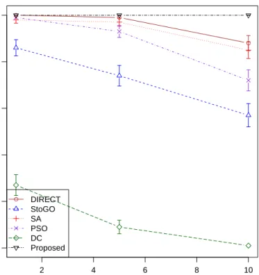
Following Section 2.2.3, we simulate 1-D signal with additive Gaussian noise, and compare the performance of the proposed algorithm with several other algorithms including DIRECT, StoGO, SA, PSO (See Section 2.4.2 for more details of these algorithms) and a recently published iterative marginal optimization (IMO) algo-rithm [41], which was specifically designed for signal and image restoration. We implement the IMO algorithm in R (see Supplementary Section A1.5 for details).

2 4 6 8 10 0 20 40 60 80 100 C P ercent success ● _● ● ● _DIRECT StoGO SA PSO DC Proposed

Figure 2.5: Comparison of different algorithms for minimizing the sum of 50 randomly generated truncated quardratic funstions in 2-D. The figure shows the mean success rates (in percents) for all the methods using 100 simulated replicates for different complexities of the functions (C). The standard errors of the means are shown as error bars.

The DC algorithm turns out to be numerically equivalent to the IMO algorithm, but much slower. Therefore, we did not include the DC algorithm in the comparison and simply named the IMO algorithm as IMO/DC.

The data are simulated by adding random Gaussian noise sampled i.i.d. from

N(0,1) to an underlying true signal. Each data set contains 100 data points equally spaced on the interval [0,1]. The true signal is design to be piece-wise smooth with different pieces being constant, linear, quadratic or sine waves (see Figure 2.6). All the algorithms are used to restore the signal by minimizing the following objective function, ˆ y= arg min ˆ y d X i=1 (ˆyi−yi)2+w d−1 X i=1 min{(ˆyi−yˆi+1)2, λ},

0.0 0.2 0.4 0.6 0.8 1.0 −5 0 5 10 x y 0.0 0.2 0.4 0.6 0.8 1.0 −5 0 5 10 x y

Figure 2.6: Simulated random signal (left) and restored signal (right) are shown in solid lines. The underlying true signal are shown in dashed lines.

point i, respectively. That is, we are solving the sum of 199 truncated quadratic functions (99 of them are truncated at λ, and the remaining 100 of them are trun-cated at infinity) in a 100-dimensional parameter space. The tuning parameters are empirically set as w= 4 and λ= 9, respectively.

We measure the performance of these algorithms using four different metrics:

1. Success rate, which is defined in Section 2.4.2. Note a success here only means that a given algorithm has found the best solution among all algorithms, which may or may not be the global minimizer.

2. Relative loss, which is defined as |f(ˆy)−f(y∗)|/|f(y∗)|, where ˆy and y∗ are the solution found by a given algorithm and the best solution found by all algorithms, respectively.

3. Root mean square error (RMSE), which is defined as

q

d−1Pd

i=1(ˆyi−y˜i)2,

where ˆy and ˜y are the solution found by a given algorithm and the underlying true signal, respectively.

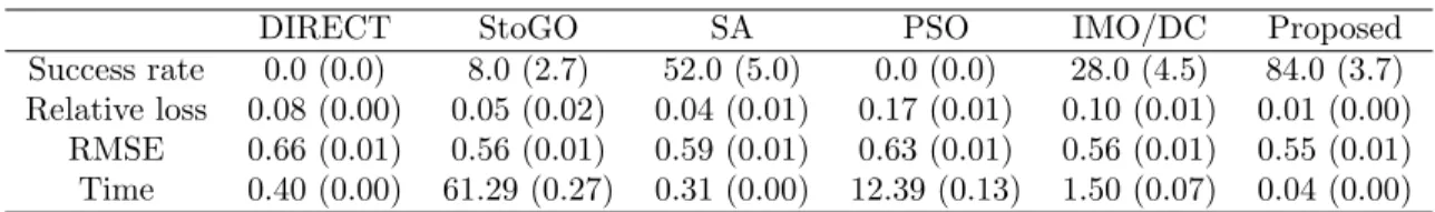
Table 2.1: Comparison of different algorithms for signal restoration. The table shows the mean success rates (in percents), relative losses, root mean square errors (RMSE), as well as running times (in seconds) for all the methods using 100 simulated replicates. The standard errors of the means are given in parentheses.

DIRECT StoGO SA PSO IMO/DC Proposed

Success rate 0.0 (0.0) 8.0 (2.7) 52.0 (5.0) 0.0 (0.0) 28.0 (4.5) 84.0 (3.7) Relative loss 0.08 (0.00) 0.05 (0.02) 0.04 (0.01) 0.17 (0.01) 0.10 (0.01) 0.01 (0.00)

RMSE 0.66 (0.01) 0.56 (0.01) 0.59 (0.01) 0.63 (0.01) 0.56 (0.01) 0.55 (0.01) Time 0.40 (0.00) 61.29 (0.27) 0.31 (0.00) 12.39 (0.13) 1.50 (0.07) 0.04 (0.00)

The performance of the proposed algorithm and other competing algorithms are summarized in Table 2.1. In general, the proposed algorithm outperforms all other methods in terms of success rate, relative loss, and RMSE. It is also significantly faster than all other algorithms.

Finally, we apply the proposed algorithm for image restoration. Both synthetic and real images are used for this experiment (see Figure 2.7 and Supplementary Fig-ure A2). All images are resized to 256×256, converted to gray scale and normalized to have pixel intensity levels in [0,1]. Independent Gaussian noise sampled from

N(µ = 0, σ2 = 0.01) is added to each pixel, and the proposed algorithm is used to restore the original image via minimizing the following objective function,

ˆ z= arg min ˆ z X i∈I (ˆzi −zi)2+w X i,j∈I,i∈D(j) min{(ˆzi−zˆj)2, λ},

where zi and ˆzi, i ∈ I, are the observed and restored intensity values at pixel i,

respectively, i ∈ D(j) means that pixels i and j are neighbors of each other, and the tuning parameters are empirically set as w = 2 and λ = 0.02, respectively. From Figure 2.7 and Supplementary Figure A2, we see that compared with Gaussian smoothing, the proposed algorithm can restore the smoothness in the image while maintaining the sharp edges. Even though this problem has a dimension of d = 256×256 = 65,536 and the number of truncated quadratic functions is n = 256×

Figure 2.7: Restoration of synthetic and real images. For each row, from left to right: original image, image with Gaussian noise added, image restored using Gaussian smoothing with a 5×5 kernel and image restored using proposed algorithm.

converge.

2.5 Discussion

We know that summing convex functions together still gives us a convex function. Although simply truncating the function at a given level does not seem to add much complexity to a convex function, the sum of truncated convex functions is not neces-sarily convex, which makes this class very powerful and flexible in modeling various kinds of problems, as illustrated in several examples given in Section 2.2. Figure 2.4 further demonstrates the diverse landscape that can be achieved by a sum of trun-cated quadratic functions. This flexibility is supported by Proposition 2.4, which implies that any problem in the class of NP can be reduced to the minimization of a sum of truncated convex functions. A potential future work is to approximate a given non-convex function by a sum of truncated quadratic functions and then use our proposed algorithm to minimize it.

In the cyclic coordinate descent algorithm, instead of performing a univariate update in each round, we can also perform a bivariate update in each round using the 2-D algorithm (i.e., using a block coordinate descent algorithm), which may help increase the chance of finding the global minimizer, at the cost of more intensive computation.

Besides the applications described in this paper, minimizing a sum of truncated convex functions also has many other applications, such as detecting differential gene expression [23] (See Supplementary Section A1.1) and personalized dose finding [8]. This paper demonstrates that the proposed algorithm can be quite efficient when the truncation boundaries of the class of convex functions are simple shapes such as an ellipse and convex polygon, which cover the cases of truncated quadratic functions and truncated`1 penalty (TLP [46]). Although these functions are seemingly limited,

their applications are abundant, and we have shown only a few selected examples in this paper. In our future work, we will investigate the application of our proposed algorithm to other classes of convex functions.

R programs for reproducing the results in this paper are available at http: //www-personal.umich.edu/~jianghui/stcf/ [42]. We used Rcpp package that substantially decreased the run time of our algorithm [15, 14, 4]. We used the al-gorithm created by David Eberly (2015) to find intersections of ellipses in our 2D algorithm [13].

Integrating Poly(A) Capture and Exome Capture RNA-Seq

Data

This chapter is motivated by a project for which we need to predict one type of RNA-seq measurements from another so that data from different types of measure-ments can be combined into one analysis. An initial attempt is to use gene-wise regressions. However, as there are more than 18,000 genes, this approach leads to a large number of parameters. Also, it would take at least 30 subjects to build a simple regression while 5 to 10 subjects is the desired sample size. In this chapter, we explain the differences between the two types of RNA-seq measurements and demonstrate potential biases when the differences are not eliminated before combining the data. Then we show that by using a linear mixed model, we not only reduce the technical differences between the two types of measurements but also improve the efficiency of the prediction. Finally, we described the discovery of outliers when fitting the data to a mixed model, which leads to the third project: outlier detection for the linear mixed model.

3.1 Introduction

Measuring the amount of messenger RNA (mRNA) molecules provides proxies for gene expression levels. A common way to extract mRNA molecules is to use oligo-dT

probes targeting on the Poly(A) tails, which distinguishes mRNAs from other types of RNA molecules (Figure 3.1). This approach, however, is limited when the specimen is profoundly degraded or formalin-fixed. When the samples are degraded, mRNA molecules could lose the Poly(A) tails. On the other hand, when the specimens are formalin fixed, the adenines of the Poly(A) tails are altered such that the oligo-dT probes no longer anneal well.

A new protocol called capture RNA sequencing was developed to overcome these difficulties: instead of oligo-dT molecules, the probes are made of short sequences designed for targeted genes. [9] showed that RNAseq measurements (Figure 3.2)based on this new protocol leads to more accurate measurements when the specimens are degraded.

Despite the effectiveness of capture sequencing for degraded or formalin-fixed samples, most RNA-seq reference libraries in major databases are based on samples process by the traditional Poly(A) protocol. However, we will show that there are differences between RNA-seq measurements from these two types protocols and di-rectly combining these two types of libraries in analyses could introduce technical biases. Therefore, for studies requiring comparison with reference libraries, it would be costly to re-build these reference libraries based on capture sequencing protocol.

In this chapter, we demonstrate the differences between poly(A) libraries and CaptureSeq libraries. Then we show that the Poly(A) measurements can be pre-dicted from the CaptureSeq measurements efficiently using the linear mixed model. With the prediction model, we can eliminate technology biases and combine the cap-ture sequencing measurements from degraded or formalin-fixed samples and Poly(A) based measurements from most reference libraries for efficient data use.

Figure 3.1: mRNA isolation, adopted from [21]. In the process of RNA-seq library preparation, RNAs are first isolated from tissue samples using commercial kits. Then mRNAs are isolated from total RNAs by annealing to oligo-dT beads. rRNAs and tRNAs are washed away before mRNAs are released from the beads.

Figure 3.2: RNA-seq workflow, adopted from [27]. The purified mRNAs are first fragmented into smaller pieces and reverse-transcribed to complementary DNAs (cDNAs). After formation of one strand of cDNA, the mRNA strand is removed and replaced by another strand of cDNA to generate a double-stranded cDNAs. Each end of the double-stranded DNA is then repaired, adenylated and ligated by adaptor before being enriched by polymerase chain reaction (PCR). Once a library has passed the quality control, it can be sent to various sequencing platforms and generate read counts data.

Table 3.1: Origins of cancer tissues of the 372 patients. Tissue origins and Number of patients

Breast 67 Prostate 64 Sarcomatoid 42

Unknown 24 Skin 20 Gall Bladder 19

Lung 18 Bladder 14 Esophagus 14

Ovary 11 Pancrease 10 Colon 9

Oral 9 Other 8 Stomach 7

Parotid Gland 7 Adrenal Gland 7 Brain 6

Kidney 5 Liver 5 Testis 3

Thymus 2 Thyroid Gland 1

3.2 The Data

We received paired capture sequencing and Poly(A) RNA-seq read counts data from 372 cancer samples. There are a total of 23 types of cancers: prostate cancer and breast cancer account for 17 percents and 18 percents of the patients (Table 3.1). Of the 372 samples, 366 of them were frozen; two of them were refrigerated, and 4 were fresh. For each sample, a capture sequencing library and a poly(A) library were prepared. As the sample tissues were obtained by core needle biopsy, there were various degrees of tissue degradation. , and the RNA integrity numbers (RINs) of all 372 pairs of libraries were recorded except for 9 libraries. Figure 3.3 shows the distribution of the RINs. In general, a RIN≥7 is considered sufficient and it is often preferred to have a RIN≥ 8 [11].

For 18236 genes out of the 18955 genes, we were able to obtain information on gene lengths, lengths of sequences overlapping with those of probes, GC contents by matching Ensembl gene id in the Genome Reference Consortium Human genome build 38 (GRCh38) (Appendix, Figure 3.11). For subsequent analyses, we normalize the read data by counts per million (CPM) and take the base two logarithms.

Figure 3.3: Distribution of the RINs of 363 poly(A) libraries. Of the 363 CaptureSeq libraries, 357 had exactly the same RINs as their poly(A) counterparts. The other 6 CaptureSeq libraries had a difference from the poly(A) measurements as -2.7, -1.5, -1.1, -0.6, 0.1, and 0.7. The RINs range from 2.5 from 10 with a mean of 8.6 and a median of 9.2. The 1st and the 3rd quartiles are 8.1 and 9.6.

3.3 Evidence of differences between the two types of measurements

To investigate the differences in measurements between the poly(A) and capture sequencing libraries, we performed cluster analyses on the poly(A) and capture se-quencing log2CPM for patients with prostate cancers based on the top 50 most varied genes across the 50 libraries. The result, as shown in Figure 3.4, suggested that the mixed measurements clustered more by protocols than by individuals.

To see if there are specific genes that cause the clustering by different protocols, we used Elastic Net logistic regression to regress the two measurement types on the log2(CPM) measurements of all genes and found four genes with non-zero coefficients (Table 3.2). The classification error rate on the testing was 0.005. Gene ontology (GO) analysis for the four genes using David 6.7 found one keyword: ”UBl conjuga-tion” with a p-value of 0.03 after Benjamini-Hochberg adjustment (FDR). We also performed differential expression analysis on the two types of measurements using DESeq2 and found 14608 significant genes among a total of 18236 genes with ad-justed p-value <0.05, which suggests diffuse differences between these two types of measurements.

Finally, to confirm that without correction, the differences in measurements based on these two types of protocol would introduce biases and false positive findings, we randomly draw 25 patients’ poly(A) log₂CPM measurements out of 50 prostate can-cer patients and compare the gene expression of these 25 patients with the remaining 25 patients using the function ”limma trend”. We perform such experiment for 1000 times and record: 1. the number of significant genes in each experiment (summarized in Figure 3.5), and 2. the number of genes found to be significantly differentially expressed in more than 50 experiments (summarized in Table 3.3) out of the 1000 experiments. We repeat the same comparison between 25 randomly drawn Poly(A)

Figure 3.4: Cluster anal ys is on the paired CaptureSeq and P oly(A) log2(CPM) measuremen ts from 25 prostate cancer patien ts. Eac h ro w represen t a gene and eac h column represen t either a library of CaptureSeq ( columns with purple tags on the top) or P oly(A) (columns with orange tags on the top) measuremen ts. The genes are the top 50 most v aried genes across th e 50 libraries. W e used the Euclidean distance and the complete metho d of Hierarc hical clu sterin g on the gene s.

Table 3.2: Nonzero coefficients of the penalized regression for classifying samples from the two technologies. We tuned the Elastic Net regression model using a sequence of α(from 0 to 1, with a step of 0.1), which determined the proportion of quadratic and L1 norm in the penalty term, and 10-fold cross-validation to chooseλ. We trained the model on 272 pairs of measurements and then tested the model on the other 100 pairs. The misclassification rate on the test set is 0.005.

Coefficient / Gene Name Coefficient Value Intercept 0.17948 ENSG00000120948 0.00017 ENSG00000115760 -0.00091 ENSG00000165119 0.00048 ENSG00000197714 -0.00042

Table 3.3: Differential expression experiments of randomly drawn subjects. Number of genes found to be significantly differentially expressed for more than 50 times in a total of 1000 experiments. Poly(A) v.s. Poly(A) Poly(A) v.s. capture sequencing Poly(A) v.s. predicted Poly(A) 0 830 0

measurements and their paired capture sequencing measurements. The results sug-gest that without correction, we can have on average more than 600 falsely positive genes in each experiment and that there are about 830 genes tend to be erroneously recognized.

3.4 Converting capture sequencing measurements to Poly(A) measure-ments

As there are various differences between the two types of measurements, using these two types of measures as if they were based on the same purification protocol could introduce biases. One solution is to convert one type of measurement to the other before combining these two types of measures into the analyses. There are several factors assumed to influence the conversion, including the degree of RNA degradation, gene length, GC content, and the length of overlapping sequence be-tween the gene and the probe. However, when these factors were incorporated, the prediction accuracy was not better. This is possibly caused by measurement errors in