Grid Synchronization and Voltage Analysis Based on the Kalman Filter

Selection of our books indexed in the Book Citation Index in Web of Science™ Core Collection (BKCI)

Interested in publishing with us?

Contact [email protected]

Numbers displayed above are based on latest data collected.

For more information visit www.intechopen.com Open access books available

Countries delivered to _{Contributors from top 500 universities} International authors and editors

Our authors are among the

most cited scientists

Downloads

We are IntechOpen,

the world’s leading publisher of

Open Access books

Built by scientists, for scientists

12.2%

122,000

135M

TOP 1%

154

Grid Synchronization and Voltage Analysis

Based on the Kalman Filter

Rafael Cardoso

1

_{and Hilton Abílio Gründling}

2

1

_{Federal University of Technology – Paraná}

Energy Processing and Analysis Research Group

2

_{Federal University of Santa Maria}

Power Electronics and Control Research Group

Brazil

1. Introduction

This chapter deals with the problem of grid synchronization in the presence of several perturbations such as harmonics, voltage unbalance, measurement noise, transients and frequency deviation. The development of two synchronization structures is presented, one for single-phase systems and the other for three-phase systems. These schemes are based on the Kalman filter and all the aforementioned perturbations are incorporated, explicitly, in the problem formulation. A voltage analyser is also developed based on the three-phase synchronization structure.

Determining the phase angle of grid voltages is important for many power conditioning devices such as active power filters, reactive power compensators, uninterruptible power supplies, distributed power generation systems, among others, that must be appropriately synchronized with grid voltages. Due to the dynamic nature of the power system, the synchronization method chosen must be capable of rejecting many perturbations inherent to the system, such as harmonics, voltage sags and swells, imbalance, frequency deviations, measurement noise and phase angle jump (Svensson, 2001; Karimi-Ghartemani & Iravani, 2004; Blaabjerg et al., 2006).

A traditional approach to the extraction of the phase angle is the use of closed-loop techniques, such as Phase-Locked Loops (PLLs) (Hsieh & Hung, 1996). For three-phase applications, the phase angle is usually obtained by means of the well-known synchronous reference frame PLL. Implementation of these methods is straightforward but they suffer from the presence of harmonics and voltage imbalance as described in (Chung, 2000). Further analysis of the behaviour of the synchronous reference frame PLL under distorted and unbalanced utility conditions can be found in (Kaura & Blasko, 1997), where some tuning recommendations are also made to minimize the impact of the harmonics and voltage unbalance in phase angle tracking. In (Timbus et al., 2006), an improved PLL, based on a repetitive controller, is proposed. This PLL has a simple structure and is capable of rejecting the negative sequence.

Another closed-loop approach is the Enhanced Phase-Locked Loop (EPLL) (Karimi-Ghartemani & Iravani, 2004). This structure is based on use of the gradient method and

Open

Access

Database

www.intechweb.org

three gains are used to tune the algorithm. Like the PLL, the choice of its gains will influence its tracking capability. Since there is no rule to guide the choice of gains, tuning them by trial and error can be tedious. The concept of the EPLL is further elaborated in (Rodríguez et al., 2006) and a new Dual EPLL (DEPLL) is discussed. According to the authors, the DEPLL can lead to detection errors under certain grid conditions. The Dual Second Order Generalized Integrator-Frequency Locked Loop (DSOGI-FLL) was later proposed to overcome the drawbacks of the DEPLL.

Open-loop techniques have also been described in the literature. In (Song & Nam, 2000) an approach based on weighted least-squares that is capable of rejecting the effects of the negative-sequence and of accommodating frequency variations is proposed. However, it is sensitive to the presence of noise and harmonics in the voltages and presents long transients in detecting frequency variations. Another simple method is the PLL based on low-pass filters (LPF-PLL) (Svensson, 2001). This method is simple but has shortcomings. The filtering process introduces a phase shift that must be compensated by a rotation matrix. The phase shift is a function of the frequency and, since this method does not consider frequency variations, full compensation of the phase shift is not possible. Voltage imbalance is also not considered and there must be a trade-off between harmonic rejection and convergence speed, defined by the cut-off frequency of the low-pass filters. Because of oscillatory behaviour, its use is not recommended for systems subjected to phase jumps (Svensson, 2001). The Normalized Positive Synchronous Frame (NPSF) is another synchronization method that is also based on low-pass filters and considers voltage imbalance and frequency deviations (De Camargo & Pinheiro, 2006). In this method, the cut-off frequency of the low-pass filters tracks the grid frequency based on an adaptation algorithm. The main drawback is that the only tuning parameter is the convergence rate of the frequency identifier. Neither the convergence speed nor harmonic rejection can be modified since the cut-off frequencies of low-pass filters must be the same as the grid frequency.

A possible alternative to extract the phase angle of a signal is the use of the Kalman filter (Kalman, 1960). This filter is well known due to its ability to deal with linear systems corrupted by uncertainties in the states of the plant as well as measurement noise. The spectrum of this type of noise is usually distributed over a wide range of frequencies which can be modelled as white noise (Gelb et al., 1996). The elimination of this perturbation by traditional filtering methods is not straightforward because of the significant phase changes that the signal can suffer. Since the Kalman filter is an optimal algorithm that considers this type of perturbation in its formulation, it is a promising alternative for extracting the phase information from a noisy signal of interest.

Some authors have studied the relation between the Kalman filter and PLL (Gupta, 1975; Christiansen, 1994; Driessen 1994; Patapounian, 1999; Izadi & Leung, 2002). Synchronization methods based on the Kalman filter are mostly used in telecommunication systems and do not consider the presence of disturbances in the signal of interest, such as harmonics and voltage sags and swells that occur in the power system; nor are they appropriate for three-phase systems. Another approach is the use of the extended Kalman filter (Svensson, 2001). However, the extended Kalman filter uses linearizations around the estimates provided by the filter. Since the linearizations are applied using the last available estimate, the propagation equations are only valid if the estimate is not very distant from the actual state (Boutayeb et al., 1997). Moreover, an arbitrary choice of filter covariance matrices together with initial filter states not sufficiently close to the actual states may lead to a filter that fails to converge (Boutayeb et al., 1999).

This chapter describes single and three-phase synchronization methods based on the Kalman filter. They are termed the Kalman Filter-Phase Locked Loop (KF-PLL) and were first introduced in (Cardoso et al., 2006) with further developments presented in (Cardoso et al., 2008). As will be shown, the Kalman gain can be evaluated off-line, so that the filter can be implemented using fixed gains, simplifying its digital implementation. The proposed method is capable of generating synchronization signals even with input signals that contain harmonics and measurement noise. To achieve this, a mathematical model that considers the existence of harmonics in the signal, and also allows for the possible occurrence of transient voltages is used. As this model involves the grid frequency, the performance of the filter may be reduced if the grid frequency deviates from the value considered in the filter. Therefore, the fundamental grid frequency is also identified and is used to update the mathematical model used in the filter. The identification procedure is based on the internal model principle (Francis & Wonham, 1976) in a way similar to that presented in (Brown & Zhang, 2004). However, the present identification method uses a modified input signal and, in contrast to (Brown & Zhang, 2004), the algorithm is entirely derived in discrete form. The first discrete implementation of such an algorithm appeared in (Zhao & Brown, 2004) but their derivation is not clear. In this chapter, the discrete derivation is presented entirely for a better understanding of its discrete implementation. For the three-phase case, the possibility of voltage imbalance is also considered, and since the Kalman filter is an optimum algorithm, the results represent a good compromise between transient response and disturbance rejection. If the stochastic model of the process to be filtered is completely known, the obtained results are optimum according to several optimization criteria (Maybeck, 1979). Performance comparisons of the proposed synchronization structures with other methods presented in literature are available in (Cardoso et al., 2008). The use of the KF-PLL is also presented for purposes of voltage analysis, where several data about the grid voltages are extracted. For instance, harmonic content with their respective amplitudes, total harmonic distortion, positive, negative and zero sequence components, and further comments on synchronization with negative and zero sequences are also addressed.

This chapter is organized as follows: Section 2 presents the Kalman filter equations. Section 3 introduces the mathematical modeling of a signal with harmonics. The grid frequency identification is described in Section 4. The proposed synchronization methods are developed in Section 5. The use of the KF-PLL for voltage analysis is presented in Section 6. Digital implementation in a fixed point DSP TMS320F2812 is described in Section 7. Finally, the results of real time experiments are given in Section 8 and conclusions are presented in Section 9.

2. The Kalman filter

Consider a discrete linear dynamic stochastic system modeled by

k k k k k

Φ

x

Γ

x

₊₁

=

+

, (1) k k k k

F

x

υ

y

=

+

, (2)

1

dim

,

1

dim

,

1

dim

x

_k

=

n

×

y

_k

=

r

×

_k

=

p

×

, (3)

where _k and

υ

_k are independent Gaussian white noise sequences with means and covariances given by

{ }

{ }

i ij T j i i

E

E

=

0

,

=

Q

δ

, (4)

{ }

{ }

i ij T j i i

E

E

υ

=

0

,

υ

υ

=

R

δ

, (5)

{ }

E

{ }

E

{ }

i

j

E

_i

υ

T_j

=

0

,

_i

x

T_j

=

0

,

υ

_i

x

T_j

=

0

,

∀

,

, (6)

where

E

{}

⋅

denotes the expectation mathematical operator and

δ

_ij denotes the Kronecker Delta function. The matrices

Φ

_k,

Γ

_k and

F

_k have appropriate dimensions.

Denoting by

x

ˆ

_k+1|k the estimate of

x

_k+1 based on all the measurements up to

k

, the filtering equation as given in (Brown, 1992) is

(

| 1

)

1 | | 1

ˆ

ˆ

ˆ

_{k+ k}

=

Φ

_k

x

_kk−

+

K

_k

y

_k

−

F

_k

x

_kk−

x

(7) where

(

)

1 1 | 1 | − − −

+

=

T _k k k k k T k k k k k

Φ

P

F

F

P

F

R

K

(8)

is the Kalman gain and

T k k k T k k k k k T k k k k k k

Φ

P

Φ

K

F

P

Φ

Γ

Q

Γ

P

_+1|

=

_{| −1}

−

_{| −1}

+

(9)

is the covariance matrix of the estimation error of the vector xk+1 evaluated at time tk:

(

)(

)

{

T

}

k k k k k k k k 1|

E

+1

ˆ

+1| +1

ˆ

+1| Δ +

=

x

−

x

x

−

x

P

. (10)

The initial conditions are given by

x

ˆ

_0|−1and

P

_0|−1. Further details can be found in (Brown, 1992).

3. Describing a signal with harmonics

To use the Kalman filter presented in section 2 a mathematical model that describes the process to be filtered is needed. Thus, to obtain a mathematical model that adequately represents grid voltage dynamics, a signal that contains only the fundamental component is initially considered; harmonic components are introduced subsequently. Hence, consider a signal with amplitude

A

_k, angular frequency

ω

_k and phase

θ

_k

(

k k k

)

k k

A

t

S

=

sin

ω

+

θ

. (11) Let

(

k k k

)

k

t

A

x

k

=

sin

ω

+

θ

1 (12) and

(

k k k

)

k

t

A

x

k

=

cos

ω

+

θ

2 . (13)

Initially, consider

A

_k+1

≈

A

_k,

ω

_k+1

≈

ω

_k and

θ

_k+1

≈

θ

_k . At the time

t

_k+1

=

t

_k

+

T

_s the signal 1 + k

S

can be expressed as

(

)

(

k s

)

(

k s

)

k s k k k k k

T

x

T

x

x

T

t

A

S

k k k

ω

ω

θ

ω

ω

sin

cos

sin

2 1 1 1 1 1 ₁

+

=

=

+

+

=

_{+ + +} + (14)

where

T

_s is the sampling period. Additionally,

(

)

(

)

cos

(

)

.

sin

cos

2 1 1 1 2 1 s k s k k s k k k k

T

x

T

x

T

t

A

x

k k k

ω

ω

θ

ω

ω

+

−

=

+

+

=

_{+ +} + (15)

To model amplitude or phase variations in the signal, a perturbation vector

[

γ

₁

γ

₂

]

T_k in the system states is considered. The state-space representation of the signal then becomes

(

)

(

)

(

k s

)

(

k s

)

_{k k} s k s k k

x

x

T

T

T

T

x

x

⎥

⎦

⎤

⎢

⎣

⎡

+

⎥

⎦

⎤

⎢

⎣

⎡

⎥

⎦

⎤

⎢

⎣

⎡

−

=

⎥

⎦

⎤

⎢

⎣

⎡

+ 2 1 2 1 1 2 1

cos

sin

sin

cos

γ

γ

ω

ω

ω

ω

, (16)

[ ]

k k k

x

x

y

_⎥

+

υ

⎦

⎤

⎢

⎣

⎡

=

2 1

0

1

(17)

where

υ

_k represents the measurement noise. If there are

n

frequencies in the signal

S

_k, i. e.,

(

)

∑

=

+

=

n i i k k i k

A

_k

i

t

_k

S

1

sin

ω

θ

, (18)

the state-space representation of the signal becomes

k n n k n n k k n n

x

x

x

x

x

x

x

x

⎥

⎥

⎥

⎥

⎥

⎥

⎦

⎤

⎢

⎢

⎢

⎢

⎢

⎢

⎣

⎡

+

⎥

⎥

⎥

⎥

⎥

⎥

⎦

⎤

⎢

⎢

⎢

⎢

⎢

⎢

⎣

⎡

⎥

⎥

⎥

⎦

⎤

⎢

⎢

⎢

⎣

⎡

=

⎥

⎥

⎥

⎥

⎥

⎥

⎦

⎤

⎢

⎢

⎢

⎢

⎢

⎢

⎣

⎡

− − + − 2 1 2 2 1 2 1 2 2 1 1 2 1 2 2 1

0

0

γ

γ

γ

γ

B

B

A

B

D

B

A

B

n 1

M

M

, (19)

[

]

k k n n k

x

x

x

x

y

+

υ

⎥

⎥

⎥

⎥

⎥

⎥

⎦

⎤

⎢

⎢

⎢

⎢

⎢

⎢

⎣

⎡

=

− 2 1 2 2 1

0

1

0

1

A

B

(20) where

(

)

(

)

(

)

(

)

⎥

⎦

⎤

⎢

⎣

⎡

−

=

s k s k s k s k

T

i

T

i

T

i

T

i

ω

ω

ω

ω

cos

sin

sin

cos

i

M

. (21)

The perturbation vector

[

γ

1

γ

2

A

γ

2_n−1

γ

2_n

]

T_k models amplitude or phase variations

of each harmonic component of the signal and its covariance is given by matrix Q, defined by (4). The covariance of the measurement noise

υ

_k is given by R as defined in (5).

The mathematical model (19)-(21) has the same form as the mathematical model (1)-(2) used in the Kalman filter. Note that this model needs the value of the angular grid frequency that may be subject to deviations from its nominal value. If the frequency considered in the mathematical model differs from the real value, the estimates provided by the filter will not be accurate. It is therefore necessary to identify the grid frequency in real time to update the model used in the Kalman filter. This is accomplished by the method given in next section.

4. Real time frequency identification

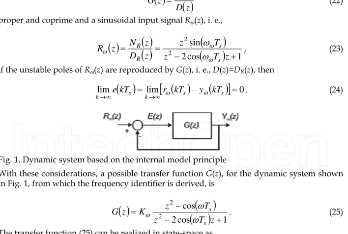
The grid frequency identification method proposed here is based on the internal model principle (Francis & Wonham, 1976), in which a stable closed-loop dynamic system is considered, as shown in Fig. 1, with

( )

_{( )}

( )

z

D

z

N

z

G

=

(22)

proper and coprime and a sinusoidal input signal Rω(z), i. e.,

( )

( )

_{( )}

(

)

(

)

1

cos

2

sin

2 2

+

−

=

=

z

T

z

T

z

z

D

z

N

z

R

s s R R ω ω ω

ω

ω

, (23)

if the unstable poles of Rω(z) are reproduced by G(z), i. e., D(z)=DR(z), then

( )

lim

[

( )

( )

]

0 lim = − = ∞ → ∞ → s k s s k kT y kT r kT e _{ω ω} . (24)

Fig. 1. Dynamic system based on the internal model principle

With these considerations, a possible transfer function G(z), for the dynamic system shown in Fig. 1, from which the frequency identifier is derived, is

( )

( )

( )

1 cos 2 cos 2 2 + − − = z T z T z K z G s s

ω

ω

ω . (25)

The transfer function (25) can be realized in state-space as

(

)

k k s k k e K x x T x x ⎥ ⎦ ⎤ ⎢ ⎣ ⎡ + ⎥ ⎦ ⎤ ⎢ ⎣ ⎡ ⎥ ⎦ ⎤ ⎢ ⎣ ⎡ − = ⎥ ⎦ ⎤ ⎢ ⎣ ⎡ + ω ω ω ω ω

ω

0 cos 2 1 1 0 2 1 1 2 1 , (26)

(

)

[

]

k k s k K e x x T y k ω ω ω ω

ω

⎥ + ⎦ ⎤ ⎢ ⎣ ⎡ − = 2 1 cos 1 (27)

where

ω

_k, at

k

=

0

, is initialized with the nominal value of the grid angular frequency. Subsequently, this value will be updated by the identification algorithm that will be developed to satisfy (24). The value of

ω

_k will be the identified grid frequency.

Let

(

_{k k}

)

k

k A tk

r_ω = _ω sin

ω

_ω +

θ

_ω (28)

be a sinusoidal reference with amplitude

k A_ω , angular frequency k ω

ω

and phase k ω

θ

at time

t

_k . Now, consider a reference as described by (28) with constant values for

k A_ω , k ω

ω

and k ω

θ

, i. e., ω ω ω A A A k k+1 = = , (29) ω ω ω

ω

ω

ω

₊ = = k k 1 , (30) ω ω ω

θ

θ

θ

₊

=

=

k k 1 (31)

and the model described by (26) and (27) with

ω

_k constant, i. e.,

ω

ω

ω

_k+1

=

_k

=

. (32) Then, if we define

(

T

s

)

( )

T

s

a

=

cos

ω

_ω

−

cos

ω

(33) and

(

T

s

)

b

=

sin

ω

_ω , (34) the state k

x

_ω2 , the output k

y

_ω and the error

e

_k will converge to

(

_ω

)

ω

ω

ω

θ

ω

ϕ

ω

A

y

t

k y

y

k

=

sin

+

+

, (35)

(

₂

)

sin

2 2 2 ω

ω

ω

θ

ω

ϕ

_ω ω k x y

t

b

a

A

x

k

+

+

+

=

, (36) and

(

ω

ω k

θ

ω

ϕ

xe_ω

)

e k

A

t

e

=

sin

+

+

, (37) respectively, where

(

)

2 2 2 2 2 2

2

K

a

K

b

b

a

K

A

A

_y ω ω ω ω ω

₊

₊

+

=

, (38)

(

)

2 2 2 2 2

2

2

b

K

a

K

a

A

A

_e ω ω ω

+

+

=

, (39)

(

)

⎟

⎟

⎠

⎞

⎜

⎜

⎝

⎛

+

+

=

2 2

2

2

arctan

b

K

a

K

ab

y ω ω ω

ϕ

, (40)

(

)

⎟⎟

_⎠

⎞

⎜⎜

⎝

⎛

+

−

=

a

K

b

K

x ω ω ω

ϕ

2

arctan

2 (41) and

(

)

⎟

⎟

_⎠

⎞

⎜

⎜

⎝

⎛

+

−

=

₂

2

arctan

a

K

ab

K

e x ω ω ω

ϕ

. (42)

When the angular frequency of the driving signal is the same as the frequency considered in the state space representation of

G

( )

z

, i. e., when

ω

_ω

=

ω

,

k

y

_ω will track the input signal

k

r

_ω by virtue of (35). Hence, from (37), in steady-state,

e

_k

=

0

. Therefore, the error

e

_k

provides useful information for the identification of the angular frequency

ω

_ω of the driving signal.

For the proposed discrete model (26)–(27), considering

ω

_ω

≈

ω

, in steady-state, two orthogonal signals are obtained,

(

ω ω

)

ω ω ≈ A

ω

tk +

θ

y k sin (43) and

( ) (

ω ω

)

ω ω ω ≈−

_ω

ω

tk +

θ

A x k _sin cos 2 . (44) Defining

φ

_k as ω ω

θ

ω

φ

_k = t_k + (45)

then, the frequency

ω

_ω can be obtained by

s k k T

φ

φ

ω

_ω = +1− ₍₄₆₎

Using (43) and (44) leads to

( )

(

₍

)

₎

₍

₎

k k x T y t t s k k k 2 sin cos sin tan ω ω ω ω ω ω ω

ω

θ

ω

θ

ω

φ

− = + + = , (47) which gives

( )

(

k

)

k

φ

φ

=arctan tan (48)

To obtain tan

( )

φ

_k in (47), we need to know the angular frequency

ω

_ω of the driving signal, which is unknown. By putting

ω

_ω ≈

ω

,

ω

_ω is replaced by

ω

. Hence,

( )

_{( )}

k k x T y s k 2 sin tan ω ω

ω

φ

− ≈ (49) and

( )

⎟

⎟

_⎠

⎞

⎜

⎜

⎝

⎛

−

≈

k k

x

T

y

s k 2

sin

arctan

ω ω

ω

φ

. (50)

Instead of using (46) to obtain the derivative of

φ

_k, (48) is used together with the definition of the continuous derivative of arctan. Then, the continuous values are replaced by the discrete ones available at time

t

_k, with continuous derivatives approximated by

( ) ( )

( )

s k k

T

dt

d

_⋅

_≈

⋅

₊₁

−

⋅

. (51)

The derivative of arctan is given by

( )

( )

[

]

( )

( )

dt

( )

( )

t

d

t

t

dt

d

_φ

φ

φ

tan

tan

1

1

tan

arctan

2

+

=

. (52)

which, by replacing

tan

( )

φ

( )

t

by its value at time

t

_k as given by (49), using (26)–(27) and re-introducing the subscript of time

k

, gives an estimate of the frequency

ω

_ω of the driving signal denoted by k ω

ω

ˆ _,

(

)

(

)

[

] [ ]

2 2 2 2

sin

sin

1

ˆ

k k k k

y

x

T

e

x

T

K

T

s k k s k s k ω ω ω ω ω

ω

ω

ω

ω

+

−

≈

(53)

giving the error _k

k

ω

ω

ˆ_ω − _,

(

)

(

)

[

] [ ]

k s s k k s k s k

T

y

x

T

e

x

T

K

T

k k k k

ε

ω

ω

ω

ω

ω ω ω ω ω

1

sin

sin

1

ˆ

2 2 2 2

₌

₋

+

−

≈

−

(54) where

(

)

(

)

[

] [ ]

2 2 2 2

sin

sin

k k k

y

x

T

e

x

T

K

s k k s k k ω ω ω ω

ω

ω

ε

+

=

. (55)

Therefore,

ω

_k can be updated by

k s u s k k

T

K

T

ε

ω

ω

₁

1

−

=

−

+ ₍₅₆₎

giving k u k k

ω

K

ε

ω

₊₁

=

−

(57)

where

K

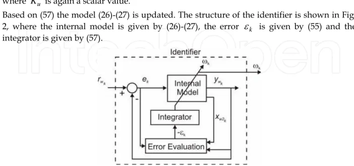
_u is again a scalar value.

Based on (57) the model (26)-(27) is updated. The structure of the identifier is shown in Fig. 2, where the internal model is given by (26)-(27), the error

ε

_k is given by (55) and the integrator is given by (57).

Fig. 2. Complete structure of the frequency identifier with signals involved.

Since the voltage measurements may be corrupted by measurement noise and harmonics and suffer from voltage sags and swells, the use of these measurements directly as

k

r

_ω may result in undesirable behavior of the frequency identifier. To avoid this, the synchronization signal is used, which is generated by the structures proposed in the next section. As will be shown, these signals are already filtered and normalized.

5. Synchronization methods

5.1 Single-phase synchronization

For single-phase synchronization, it is necessary to generate a signal in phase with the fundamental component of the grid voltage. From (19), it is clear that

(

_k

)

k Ak ktk x1 = sin

ω

+

θ

1 (58) and

(

_k

)

k

A

k k

t

k

x

₂

=

cos

ω

+

θ

₁ , (59)

are the orthogonal components of the fundamental voltage phasor of the grid voltage. Its instantaneous phase is

k k k k

V1

ω

t

θ

1

φ

= + . (60)

From the Kalman filter described in section 2, with a mathematical model of the signal

S

_k

given by (19)–(21), the estimates of the components of the fundamental voltage phasor

1 | 1

ˆ

− k k

x

and 1 | 2

ˆ

− k k

x

are obtained. Based on these estimates, and assuming

A

_k

≠

0

, the sine and cosine functions are given by

( )

kk _k k

_A

r

x

k V ω

φ

=

1| −1

=

1

ˆ

sin

(61) and

( )

k V

A

x

k k k 1 | 2 1

ˆ

cos

φ

=

− (62) where 2 2 2 1| 1

ˆ

| 1

ˆ

− −

+

=

k k k k

x

x

A

_k . (63)

The angular frequency

ω

_k needed in the mathematical model used by the Kalman filter is updated by the algorithm described in section 4. The reference signal

k

r_ω is obtained from (61). This signal contains only the fundamental component of the measured signal and is normalized. The influence of harmonics or amplitude variations of the measured signal is therefore minimized. Fig. 3 shows the proposed single-phase synchronization structure. In this figure, the block termed the Kalman Filter is implemented by (7)–(9). The input of the filter, that is,

y

_k in (7), is the voltage measurement of the phase of interest. In Fig. 3, the input of the filter is represented by

v

_k. The Kalman filter will provide the estimates of the harmonics included in the mathematical model (19)–(21) used to describe the signal. Since the interest is on the fundamental component, only the first two estimated states

1 | 1

ˆ

− k k

x

and 1 | 2

ˆ

− k k

x

are used. These estimates are the two orthogonal signals used to obtain the synchronization signals as depicted in Fig. 3.

Fig. 3. Single-phase synchronization structure.

From (61) and (62) the instantaneous phase of the fundamental grid voltage component is found to be

⎟

⎟

⎠

⎞

⎜

⎜

⎝

⎛

=

− − 1 | 1 | 2 1 1

ˆ

ˆ

arctan

k k k k k

_x

x

V

φ

. (64) 5.2 Three-phase synchronization

In some applications, such as power conditioning equipment (Campos et al., 1994; Song & Nam, 2000), distributed generation (Karimi-Ghartemani & Iravani, 2004; Blaabjerg et al., 2006), PWM rectifiers (De Camargo & Pinheiro, 2006) among others, it is desirable that the synchronization method be able to provide synchronism signals in phase with the positive sequence of the fundamental component of the grid voltages.

Given the fundamental phase voltages _af k

v

, _bf k

v

and _cf k

v

, the positive sequence components can be obtained through (Fortescue, 1918)

k f c f b f a k c b a

v

v

v

v

v

v

⎥

⎥

⎥

⎦

⎤

⎢

⎢

⎢

⎣

⎡

⎥

⎥

⎥

⎦

⎤

⎢

⎢

⎢

⎣

⎡

=

⎥

⎥

⎥

⎦

⎤

⎢

⎢

⎢

⎣

⎡

+ + +

1

1

1

3

1

2 2 2

α

α

α

α

α

α

(65) where

α

=

e

j120c . Considering

e

j120c

( )

1

₂

3

₂

⎟

e

j90c

⎠

⎞

⎜

⎝

⎛

±

−

=

±

and defining

S

₉₀ as the

90

c

phase shift operator, i. e.,

S

₉₀

=

e

j90c , (65) can be rewritten as

(

)

(

)

(

)

(

)

.

6

3

6

1

3

1

,

,

6

3

6

1

3

1

90 90 f b f a f b f a f c c c a b f c f b f c f b f a a k k k k k k k k k k k k k k k

v

v

S

v

v

v

v

v

v

v

v

v

S

v

v

v

v

−

+

+

−

=

−

−

=

−

+

+

−

=

+ + + + + (66) The values of _af k

v

, _bf k

v

, _cf k

v

and their orthogonal components

( )

_af

k

v

S

₉₀ ,

( )

_bf k

v

S

₉₀ and

( )

f ck

v

S

₉₀ are obtained directly from the Kalman filter due to (58) and (59). That is, a f ak

x

kk

v

1 | 1

ˆ

−

=

, _bf b k k k

x

v

1 | 1

ˆ

−

=

, _cf c k k k

x

v

1 | 1

ˆ

−

=

and

( )

_af a k k k

x

v

S

1 | 2 90

=

ˆ

₋ ,

( )

b f bk

x

kk

v

S

1 | 2 90

=

ˆ

₋ ,

( )

f c ck

x

kk

v

S

1 | 2

90

=

ˆ

₋ , where the superscripts a, b and c indicate the filter associated to each

phase. This avoids the need for additional filters to provide the phase shift required in the fundamental component to obtain the orthogonal components of the voltages.

To obtain the synchronism signals, the positive sequence components are represented in the stationary reference frame

αβ

:

k c b a k

_v

v

v

v

v

⎥

⎥

⎥

⎦

⎤

⎢

⎢

⎢

⎣

⎡

⎥

⎥

⎦

⎤

⎢

⎢

⎣

⎡

−

−

−

=

⎥

⎥

⎦

⎤

⎢

⎢

⎣

⎡

+ + + + +

2

3

2

3

0

2

1

2

1

1

3

2

β α . (67)

To simplify the transforms (66) and(67), they can be combined as

f abc 2 f abc 1 α

T

v

T

v

v

k k

+

S

90

=

+ (68) where k f c f b f a k

_v

v

v

v

v

k k

⎥

⎥

⎥

⎦

⎤

⎢

⎢

⎢

⎣

⎡

=

⎥

⎥

⎦

⎤

⎢

⎢

⎣

⎡

=

₊+ + f abc α

v

v

,

β α , (69)

⎥

⎥

⎦

⎤

⎢

⎢

⎣

⎡

−

−

−

=

4

3

4

3

0

4

1

4

1

2

1

3

2

1

T

, (70) and

⎥

⎥

⎦

⎤

⎢

⎢

⎣

⎡

−

−

−

=

4

1

4

1

2

1

4

3

4

3

0

3

2

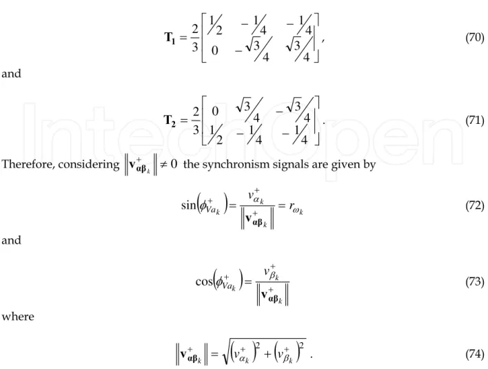
2

T

. (71) Therefore, considering +

≠

0

k α

v

the synchronism signals are given by

( )

_k k k k

r

v

Va ω α

φ

=

₊

=

+ + α

v

sin

(72) and

( )

₊+ +

₌

k k k

v

Va α

v

β

φ

cos

(73) where

( ) ( )

₊ 2 ₊ 2 +

₌

₊

k k k

v

α

v

β α

v

. (74)

The angular frequency in the mathematical model used by the Kalman filter is updated again by the algorithm set out in section 4. The reference signal

k

r

_ω is obtained from (72). Fig. 4 shows the proposed three-phase synchronization method. Similar to the single-phase case, the signals

k a

v

, k b

v

and k c

v

, in Fig. 4, are the inputs of three Kalman filters used to decompose the grid voltages of each phase in the harmonic components considered in the signal model. From each filter, the first two orthogonal estimated states are used by the positive sequence extractor block, i. e., _af

k

v

, _bf

k

v

, _cf

k

v

and its orthogonal components

( )

f ak

v

S

₉₀ ,

( )

_bf k

v

S

₉₀ and

( )

_cf k

v

S

₉₀ . Note that to reduce the processing time, the positive sequence extractor and abc to

αβ

blocks are combined as shown by (68).

The instantaneous phase can be obtained from (72) and (73),

⎟

⎟

⎠

⎞

⎜

⎜

⎝

⎛

=

₊ + + k k k

v

v

Va β α

φ

arctan

(75)

while the amplitude of the positive sequence component is

+ +

₌

k k

A

v

_α . (76)

6. Voltage analysis

In Fig. 4, which shows the structure of the three-phase KF-PLL, it can be observed that some information about the grid voltages can be directly obtained, for instance, fundamental components, harmonics, symmetrical components and frequency. This indicates that the KF-PLL can also be used for purposes of voltage analysis. This section describes how the information provided by the different blocks of the KF-PLL can be used for this purpose. The three-phase KF-PLL uses three Kalman filters in its first block. Each filter is associated to one of the phase voltages. Based on these filters, it is possible to optimally extract the harmonics of each phase voltage and their orthogonal components. Hence, the amplitude of the considered harmonic component can be obtained straightforwardly as shown by (58), (59) and (63). In this case, the fundamental component was considered. Obviously, it can be extended to any harmonic component considered in the model (19)-(21).

Based on the harmonic components extracted by the Kalman filters, the total harmonic distortion (THD) can also be evaluated in real time, that is,

k n i i k

A

A

THD

k

∑

=

=

2 2 (77)

where

A

_k is the amplitude of the fundamental component and

k

i

A

is the amplitude of the i-th harmonic component.

The detection of the symmetrical components is important for purposes of monitoring unbalance. In the KF-PLL, the positive sequence is promptly available. To measure the degree of unbalance, the negative and possibly the zero sequence components must be also detected. The zero sequence component can be obtained from

)

(

3

1

0 f c f b f a k

v

_k

v

_k

v

_k

v

=

+

+

_{, (78)}

while its magnitude can be evaluated from

( ) ( )

₀ 2 90 2 0 0 k k k

v

S

v

A

=

+

(79) where

)

(

3

1

90 90 90 0 90 f c f b f a k

S

v

_k

S

v

_k

S

v

_k

v

S

=

+

+

. (80)

The negative sequence components are obtained straightforwardly from

c

b

a

i

v

v

v

v

_{i i}f _{i k} k k k

,

,

,

0

₌

−

−

=

+ − , (81)

while its magnitude is given by

( ) ( ) ( )

⎟

_⎠

⎞

⎜

⎝

⎛

₊

₊

=

− − − − 2 2 2

3

2

k k k b c a k

v

v

v

A

. (82)

Note that representing the negative sequence components in the

αβ

reference frame, that is,

k c b a k

_v

v

v

v

v

⎥

⎥

⎥

⎦

⎤

⎢

⎢

⎢

⎣

⎡

⎥

⎥

⎦

⎤

⎢

⎢

⎣

⎡

−

−

−

=

⎥

⎥

⎦

⎤

⎢

⎢

⎣

⎡

− − − − −

2

3

2

3

0

2

1

2

1

1

3

2

β α , (83)

the synchronization signals with these components can be obtained by

( )

( )

₋− − − − −

₌

₌

k k k k k k

v

v

Va Va α α

v

v

β α

_φ

φ

,

cos

sin

(84) where

( ) ( )

₋ 2 ₋ 2 − −

₌

₌

₊

k k k

A

k

v

α

v

β α

v

. (85)

Hence, the instantaneous phase of the negative sequence component is

⎟

⎟

⎠

⎞

⎜

⎜

⎝

⎛

=

₋ − − k k k

v

v

Va β α

φ

arctan

. (86) Similarly,

( )

( )

₀0 90 0 0 0

cos

,

sin

k k Va k k V

A

v

S

A

v

k k

=

=

−

φ

φ

(87)

And the instantaneous phase of the zero sequence component is given by

⎟

⎟

⎠

⎞

⎜

⎜

⎝

⎛

=

₀ 90 0 0

arctan

k k V

v

S

v

k

φ

. (88)

Further details on voltage analysis based on Kalman filter can be found in (Cardoso et. al., 2007).

7. Digital implementation

This section describes the digital implementation of the synchronization methods in a 32 bits fixed-point DSP (TI-TMS320F2812). Because of the finite word length and precision of the device, the IQmath library (Texas Instruments, 2002) was used to improve the performance of the algorithms. To determine the sampling frequency, two factors must be considered: calculation time and the sampling frequency usually used in the power electronic apparatus. If neither the calculation time nor the equipment sampling frequency impose restrictions, higher sampling frequencies will provide better results. The sampling frequency used here is 10.5 kHz.

The mathematical model used in the Kalman filter incorporates the fundamental, 3rd_{, 5}th_{, 7}th

and 11th _{harmonics. The covariance of the measurement noise is set to}

_R

=

₂₀₀

_V

2 _{while the}

covariance of the process noise is set to

Q

=

0

.

05

I

_10×10

V

2. In fact, in practice, both matrices

Q

and

R

can be identified by using whitening techniques as presented in (Mehra, 1970; Cardoso et al., 2005).

To design the transfer function gain

K

_ω, see (25), the natural frequency is set equal to the nominal angular frequency of the grid, i. e.,

ω

_n

=

ω

=

377

rad

/

s

and a damping coefficient

707

.

0

=

ξ

is used. Therefore, from the well known relationships (Ogata, 1994)

n s T

e

z

=

− ξω (89) and

)

(

1

2

rad

T

z

=

_s

ω

_n

−

ξ

∠

(90)

replacing the values of

ω

_n and

ξ

by those defined for them gives the roots of the closed loop characteristic equation, i. e.,

025

.

0

975

.

0

j

z

=

±

. (91)

From (91) and the closed loop characteristic equation, solving for

K

_ω we have

K

_ω

=

0

.

052

. The gain

K

_u is responsible for the speed of convergence of the frequency identifier. For fast convergence,

K

_u must have a large value. However, a high value for

K

_u may lead to an undesirable behavior of the identifier. In the following experiments

K

_u

=

20

. This gain provides a satisfactory performance for the integrator.

When implementing the Kalman filter, it is necessary to evaluate the Kalman gain Kk, given

by (8), for which the covariance matrix (9) must be computed at every sampling time k. Since the standards (IEC 60034, 1996; IEC 61000-2-2, 2001; IEEE Std C37.106, 2003) limit the range of frequency deviation in the grid, a fixed Kalman gain can be evaluated at the nominal grid frequency. This simplification imposes a negligible reduction in the performance of the Kalman filter when compared with the use of the Kalman gain evaluated for the actual grid frequency, as will be shown below.

Considering

f

=

60

Hz

and based on the values

Q

=

0

.

05

I

_10×10

V

2 and

R

=

200

V

2, previously defined, the following steady-state Kalman filter gain is obtained

[

]

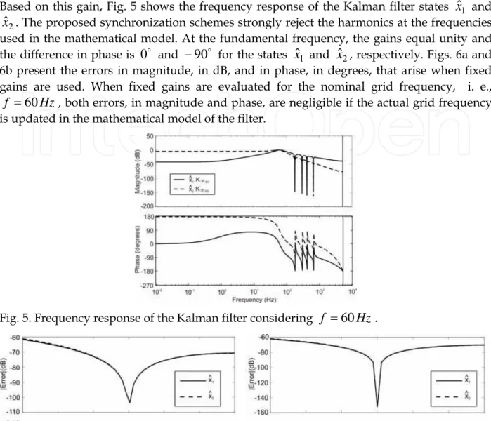
₁₀ 3 2893 . 2 0486 . 21 5481 . 1 1161 . 21 0693 . 0 1727 . 21 1728 . 0 1721 . 21 0848 . 0 1726 . 21 60 − ∞ × − − − = T A A K . (92)

Based on this gain, Fig. 5 shows the frequency response of the Kalman filter states

x

ˆ

₁ and

2

ˆ

x

. The proposed synchronization schemes strongly reject the harmonics at the frequencies used in the mathematical model. At the fundamental frequency, the gains equal unity and the difference in phase is

0

c and

−

90

c for the states

_x

ˆ

_{1 and}

_x

ˆ

_{2, respectively. Figs. 6a and} 6b present the errors in magnitude, in dB, and in phase, in degrees, that arise when fixed gains are used. When fixed gains are evaluated for the nominal grid frequency, i. e.,

Hz

f

=

60

, both errors, in magnitude and phase, are negligible if the actual grid frequency is updated in the mathematical model of the filter.

Fig. 5. Frequency response of the Kalman filter considering

f

=

60

Hz

.

a) Error introduced by using fixed Kalman gains but considering

f

=

57

Hz

in the mathematical model of the Kalman filter.

b) Error introduced by using fixed Kalman gains but considering

f

=

63

Hz

in the mathematical model of the Kalman filter. Fig. 6. Frequency response errors for different conditions of operation of the Kalman filter.

8. Experimental results

The single and three-phase synchronization methods were implemented in a fixed point DSP (TI-TMS320F2812) to evaluate their performance in real time. The Kalman gain used and sampling frequency are the same as described in section 7. Fig. 7a and Fig. 7b depict the synchronization signals obtained with the proposed single and the three-phase KF-PLLs

superimposed with the distorted grid voltage (

THD

=

5

.

8

%

).Fig. 7c and Fig. 7d show the synchronization signals for a sinusoidal grid voltage. The good behavior of both proposed structures can be noted, even when voltage waveforms are distorted.

a) Single-phase under distorted grid voltages (THD=5.8%)

b) Three-phase under distorted grid voltages (THD=5.8%)

c) Single-phase under sinusoidal grid voltages

d) Three-phase under sinusoidal grid voltages Fig. 7. Synchronization signals obtained.

The use of the KF-PLL for purposes of voltage analysis is exemplified in the following set of experimental results. Again, the results are based on a fixed point DSP (TI-TMS320F2812) implementation. The voltages are composed of a 220 V fundamental component and the following harmonics are present: 5th_{, 7}th_{, and 11}th_{, with amplitudes given by 0.3 p.u., 0.15}

p.u. and 0.09 p.u., respectively, referring to the fundamental peak value. Therefore, the total harmonic distortion of the voltages is

THD

=

34

.

7

%

. At

t

=

0

.

0832

s

a voltage drop of 30% occurs in all phases. Additionally, an unbalance of 50% is considered in phase c. The KF-PLL was tuned considering: Q=0.01I_10×10V2 ,

R

=

20

V

2,

Ku

=

20

and

Kw

=

0

.

052

.

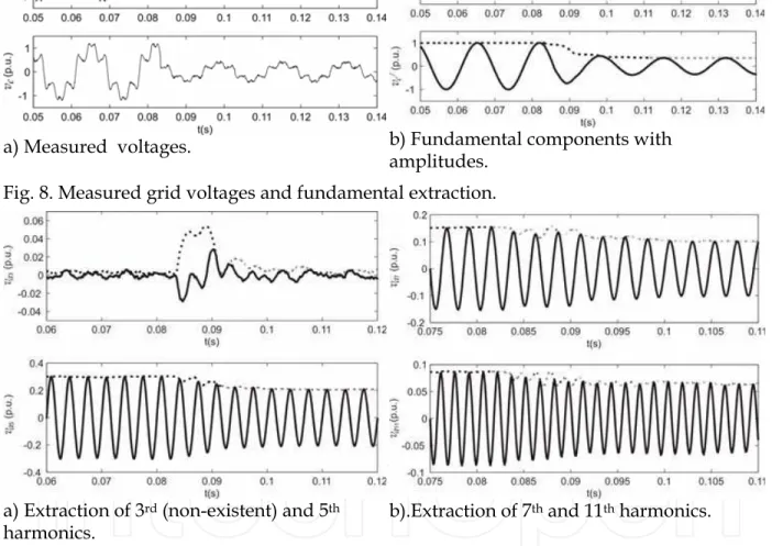
Fig. 8a shows the measured grid voltages while Fig 8b depicts the extracted fundamental components of each phase with their amplitudes. Note that the fundamental components are adequately detected. The same occurs with the peak values. The convergence of the signals is fast and occurs in less than one cycle.

Fig. 9 presents the extraction of the harmonics in the measured signal with their amplitudes evaluated in real time. Note that the non-existent 3rd harmonic is also correctly detected.

a) Measured voltages. b) Fundamental components with

amplitudes. Fig. 8. Measured grid voltages and fundamental extraction.

a) Extraction of 3rd _{(non-existent) and 5}th

harmonics.

b).Extraction of 7th _{and 11}th _harmonics.

Fig. 9. Harmonic decomposition and amplitude detection.

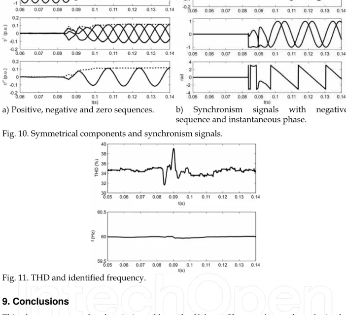
The detection of the symmetrical components is depicted in Fig. 10a. Until t=0.0832s the grid voltages are balanced and the negative and zero sequence are zero. After t=0.0832s, the voltages are unbalanced and the proposed method detects the presence of negative and zero sequences adequately. The amplitude of the positive, negative and zero sequences are also correctly identified.

Fig. 10b shows the generation of the synchronization signals with the negative sequence components of the fundamental voltages. It also presents the associated instantaneous phase. Similar results can also be obtained with the zero sequence component or any harmonic signal of interest.

Finally, Fig. 11 depicts the THD of the phase a voltage, evaluated in real time. It also shows the identified grid frequency, which due to the normalized signal used to drive the identifi_{er, is practically immune to transients in grid voltages.}

a) Positive, negative and zero sequences. b) Synchronism signals with negative sequence and instantaneous phase.

Fig. 10. Symmetrical components and synchronism signals.

Fig. 11. THD and identified frequency.

9. Conclusions

This chapter presented a description of how the Kalman filter can be used to obtain the synchronization signals with the grid voltages as well as how it can also be helpful for voltage analysis. As for synchronization, the described methods are capable of dealing with signals corrupted by harmonics and measurement noise. For three-phase systems the method also considers voltage imbalance.

To deal with voltage frequency variations, the fundamental grid frequency is identified in real time to update the Kalman filter model. It was shown that for frequency deviations within the limits allowed by several standards, fixed Kalman gains can be used, which simplifies digital implementation. The formulation of the proposed synchronization schemes deals explicitly with the following phenomena that can occur in a real system: presence of harmonics, voltage transients, measurement noise, voltage imbalance and frequency deviation.

As mentioned, the synchronization methods can also provide information about the grid voltages such as harmonic analysis, amplitude detection, instantaneous phase, extraction of symmetrical components and frequency, useful for the analysis of power quality.

The experimental results show that the proposed synchronization methods can be implemented without great difficulty in a fixed-point DSP. The implementation based on fixed Kalman gains simplifies the DSP implementation, and it was shown that the effect on performance of the fixed gains is small.

10. References

BLAABJERG, F.; TEODORESCU, R.; LISERRE, M.; TIMBUS, A. V. (2006). Overview of control and grid synchronization for distributed power generation systems. IEEE Transactions on Industrial Electronics, Vol. 53, No. 5, October 2006, pp. 1398-1409 BOUTAYEB, M., RAFARALAHY, H., DAROUACH, M. (1997). Convergence analysis of the

extended Kalman filter used as an observer for nonlinear deterministic discrete-time systems, IEEE Transactions on Automatic Control, Vol. 42, No. 4, April 1997, pp. 581-586 BOUTAYEB, M., AUBRY, D. (1999). A strong tracking extended Kalman observer for

nonlinear discrete-time systems, IEEE Transactions on Automatic Control, Vol. 44, No. 8, August 1999, pp. 1550-1556

BROWN, R. G. (1992) Introduction to Random Signals and Applied Kalman Filtering, John Wiley & Sons, New York

BROWN, L. J., ZHANG, Q. (2004). Periodic disturbance cancellation with uncertain frequency, Automatica, Vol. 40, No. 4, April 2004, pp. 631-637

CAMPOS, A., JOOS, G., ZIOGAS, P. D., LINDSAY, J. F. (1994). Analysis and design of a series voltage unbalance compensator based on a three-phase VSI operating with unbalance switching functions, IEEE Transactions on Power Electronics, Vol. 9, No. 3, May 1994, pp. 269-274

CARDOSO, R., CÂMARA, H. T., GRÜNDLING, H. A. (2005). Sensorless induction motor control using low cost electrical sensors, Proceedings of 36th _{IEEE Power Electronics}

Specialists Conference, pp. 1600-1606, June 2005, IEEE, Recife

CARDOSO, R., DE CAMARGO, R. F., PINHEIRO, H., GRÜNDLING, H. A. (2006). Kalman filter based synchronization methods, Proceedings of 37th _{IEEE Power Electronics}

Specialists Conference, pp. 1935-1941, June 2006, IEEE, Jeju

CARDOSO, R.; KANIESKI, J. M.; PINHEIRO, H. & GRÜNDLING, H. A. (2007). Power quality evaluation based on optimum filtering theory for time-varying frequencies,

Proceedings of 9th _{Brazilian Power Electronics Conference, pp. 462-467,}

September-October 2007, Sobraep, Blumenau

CARDOSO, R.; DE CAMARGO, R. F.; PINHEIRO, H. & GRÜNDLING, H. A. (2008). Kalman filter based synchronization methods. IET Generation, Transmition & Distribution, Vol. 2, No. 4, July 2008, pp. 542-555

CHUNG, S.-K. (2000). A phase tracking system for three phase utility interface inverters.

IEEE Transactions on Power Electronics, Vol. 15, No. 3, May 2000, pp. 431-438

CHRISTIANSEN, G. S. (1994). Modelling of a PRML timing loop as a Kalman filter,

Proceedings of IEEE Global Telecommunications Conference, pp. 1157-1161, November-December 1994, IEEE, San Francisco

DE CAMARGO, R. F., PINHEIRO, H. (2006). Synchronization method for three-phase PWM converters under unbalance and distorted grid. IEE Proceedings Electric Power Applications, Vol. 153, No. 5, September 2006, pp. 763-772

DRIESSEN, P. F. (1994). DPLL bit synchronizer with rapid acquisition using adaptive Kalman filtering techniques. IEEE Transactions on Communications, Vol. 42, No. 9, September 1994, pp. 2673-2675

FORTESCUE, C. L. (1918). Method of symmetrical coordinates applied to the solution of polyphase networks. Trans. AIEE, Vol. 37, 1918, pp. 1027-1140

FRANCIS, B. A., WONHAM, W. M. (1976). The internal model principle of control theory,

Automatica, Vol. 12, No. 5, 1976, pp. 457-465

GELB, A., KASPER JR., J. F., NASH JR., R. A., PRICE, C. F., SUTHERLAND JR. A. A. (1996).

Applied Optimal Estimation, M.I.T. Press, Cambridge

GUPTA, S. C. (1975). Phase-locked loops. Proceedings of the IEEE, Vol. 63, 1975, pp. 291-306 HSIEH, G.-C., HUNG, J. C. (1996). Phase-locked loop techniques-a survey. IEEE Transactions

on Industrial Electronics, Vol. 43, No. 6, December 1996, pp. 609-615

IZADI, M. H., LEUNG, B. (2002). PLL-based frequency discriminator using the loop filter as an estimator. IEEE Transactions on Circuit and Systems-II: Analog and Digital Signal Processing, Vol. 49, No. 11, November 2002, pp. 721-727

IEC 60034 (1996). Rotating electrical machines part 3: Specific requirements for turbine-type synchronous machines, IEC

IEC 61000-2-2 (2001). Electromagnetic compatibility (EMC) part 2-2: Environment-Compatibility levels for low frequency conducted disturbances and signaling in public low-voltage power supply systems, IEC

IEEE Std C37.106 (2003). IEEE guide for abnormal frequency protection for power generating plants, IEEE

KALMAN, R. E. (1960). A new approach to linear filtering and prediction problems. Journal of Basic Engineering, Series 82D, March 1960 , pp. 35-45

KARIMI-GHARTEMANI, M., IRAVANI, M. R. (2004). A method for synchronization of power electronic converters in polluted and variable-frequency environments. IEEE Transactions on Power Systems, Vol. 19, No. 3, August 2004, pp. 1263-1270

KAURA, V., BLASKO, V. (1997). Operation of a phase locked loop system under distorted utility conditions. IEEE Transactions on Industry Applications, Vol. 33, No. 1, January/February 1997, pp. 58-63

MAYBECK, P. S. (1979). Stochastic Models, Estimation and Control-Vol. 1, Academic Press, New York MEHRA, R. K. (1970). On the identification of variances and adaptive Kalman filtering. IEEE

Transactions on Automatic Control, Vol. AC-15, No. 3, April 1970, pp. 175-184 OGATA, K. (1994). Discrete-Time Control Systems, Prentice-Hall, Upper Saddle River

PATAPOUNIAN, A. (1999). On phase-locked loops and Kalman filters. IEEE Transactions on Communications, Vol. 47, No. 5, May 1999, pp. 670-672

RODRÍGUEZ, P., LUNA, A., CIOBOTARU, M., TEODORESCU, R., BLAABJERG, F. (2006). Advanced grid synchronization system for power converters under unbalanced and distorted operating conditions, Proceedings of Annual Conference of the IEEE Industrial Electronics Society, pp. 5173-5178, November 2006, IEEE, Paris

SONG, H.-S., NAM, K. (2000). Instantaneous phase-angle estimation algorithm under unbalanced voltage-sag conditions. IEE Proc. Gener. Transm. Distrib., Vol. 147, No. 6, November 2000, pp. 409-415

SVENSSON, J. (2001). Synchronization methods for grid-connected voltage source converters, IEE Proc. Gener. Transm. Distrib., Vol. 148, No. 3, May 2001, pp. 229-235 TEXAS INSTRUMENTS (2002). IQ Math Library-Module User’s Guide-C28x Foundation

Software, TI, Dallas

TIMBUS, A. V., BLAABJERG, F., TEODORESCU, R., LISERRE, M., RODRIGUEZ, P. (2006). PLL algorithm for power generation systems robust to grid voltage faults,

Proceedings of 37th _{IEEE Power Electronics Specialists Conference, pp. 1360-1366, June}

2006, IEEE, Jeju

ZHAO, Z., BROWN L. (2004). Fast estimation of power system frequency using adaptive internal-model control technique, Proceedings of 43rd _{IEEE Conference on Decision and}