Learning from the Mistakes of Others:
Matching Errors in Cross-Dataset Learning
Viktoriia Sharmanska and Novi Quadrianto
SMiLe CLiNiC, University of Sussex, Brighton, UK
[email protected]; [email protected]Abstract
Can we learn about object classes in images by looking at a collection of relevant 3D models? Or if we want to learn about human (inter-)actions in images, can we bene-fit from videos or abstract illustrations that show these ac-tions? A common aspect of these settings is the availabil-ity of additional or privileged data that can be exploited at training time and that will not be available and not of inter-est at tinter-est time. We seek to generalize the learning with priv-ileged information (LUPI) framework, which requires addi-tional information to be defined per image, to the setting where additional information is a data collection about the task of interest. Our framework minimizes the distribution mismatch between errors made in images and in privileged data. The proposed method is tested on four publicly avail-able datasets: Image+ClipArt, Image+3Dobject, and Im-age+Video. Experimental results reveal that our new LUPI paradigm naturally addresses the cross-dataset learning.
1. Introduction
Vapnik et al. [35, 24, 34] introduced learning with
privileged information (LUPI) as a learning with teacher paradigm, where at the training stage, a teacher gives some
additionalexplanationx⋆
i about an examplexi. LUPI has
been shown useful in a variety of learning scenarios such as
ranking [28], categorization [37], structured prediction [9],
data clustering [8], metric learning [10], face/gesture
recog-nition [38], glaucoma detection [7], and recently learning
with annotation disagreements [27]. Most LUPI methods
(e.g. [35,28,20,14]) follow the assumption that the
ex-tra information is useful to discriminate between easy and difficult examples. This knowledge is then used to deter-mine the influence of each instance in the training process. Specifically, one puts less emphasis or even ignores diffi-cult instances during training in hope that this will improve performance. Reflecting on how per-instance privileged in-formation can be used to identify whether this instance is
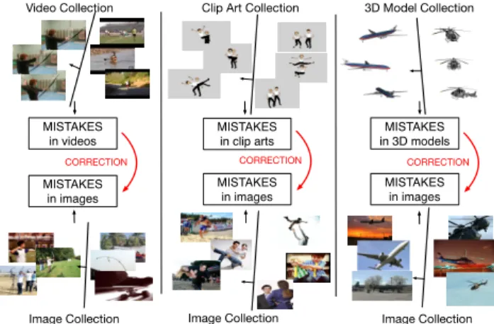
Video Collection MISTAKES in videos MISTAKES in images CORRECTION Image Collection
Clip Art Collection 3D Model Collection
MISTAKES in clip arts MISTAKES in images CORRECTION Image Collection MISTAKES in 3D models MISTAKES in images CORRECTION Image Collection
Figure 1: In this work, we propose a framework to solve
vi-sion tasksin imagesby acquiring knowledge from the
mis-takes committed by other data collections (videos, clip arts, and 3D models) when learning the same concepts.
an easy or a difficult one, we ask the following question: is
it possible to transfer easiness and hardness ina class sense
instead ofper-instance?
This paper seeks to advice the learner to acquire knowl-edge from the mistakes committed by others when learn-ing the same concept. One will learn that maklearn-ing errors on an example-by-example basis is unavoidable, but one will make the right decisions at a larger scale by minimizing di-vergence between own mistakes and others’. We will ex-plore a distribution matching over the mistakes in original and privileged representations as a principled approach to achieve the class-level information transfer. We will use the regularized risk functional framework and replace the em-pirical risk with an (emem-pirical) divergence term character-izing the mismatch between error distributions on the priv-ileged and original spaces. This approach is innovative in
two senses: (1) Prior knowledge is normally encoded in
the regularization term, instead we introduce bias into the
risk (loss) term. (2)Almost all distribution matching
meth-ods match input features and/or function outputs, instead we match error distributions.
2. Related work
In the literature, distribution matching has been proposed
for, among others, transduction learning (e.g. [25]) and
do-main adaptation (e.g. [21, 40]). Quadrianto et al. [25]
matched the distribution between function outputs on the
training data f(X) := {f(x1), . . . , f(xN)} and outputs
on the test dataf(X′) := {f(x′
1), . . . , f(x′N′)}to devise
a general transduction algorithm for classification, regres-sion, and structured prediction settings, whereas we
pro-pose to match error distributions on privileged and
origi-nal domains. The empirical Maximum Mean Discrepancy
(MMD) [12] is employed as the nonparametric metric of
difference between two distributions. In the domain
adapta-tion setting, Pan et al. [23] used the MMD metric to project
data from a target domain X := {x1, . . . ,xN} and a
re-lated source domainX′ :={x′
1, . . . ,x′N′}into a common
subspace such that the difference between the distributions of source and target domains is reduced. Recently, Zhang
et al. [40] proposed to also use the MMD metric to project
dataXandX′as well as function outputsf(X)andf(X′)
in the framework of deep neural networks.
In general, finding projection matrices involves either transformation of the data from source and target into a common subspace (two projection matrices) or transfortion of the data from source to target (one projectransfortion ma-trix). The projection methods can be expensive in both computational complexity and memory requirement (if the data dimensionality is high). Our method offers a refreshing look on domain adaptation problems that sidestep the pro-cess of finding projection matrices. The cross-dataset sce-nario in this paper overlaps with the work of, for example,
[32], which aims to overcome dataset bias across multiple
image datasets in the domain adaptation scenario. In con-trast, we explore cross-modal transfer in the cross-dataset
learning. Complementary to us, [13] recently use a
distilla-tion framework for cross-modal representadistilla-tion learning.
Modeldistillation or compression [15,2] has attracted
attention in the domain adaptation setting with deep
archi-tectures (e.g. [33,13]). The aim is to learn representations
for an unlabeled or sparsely labeled target domain by using a large labeled source domain as a supervisory signal. The framework uses output probability predictions on source domain as training labels for target domain and shows that this training is more accurate than using the original tar-get labels. Instead we propose to match error distributions across domains as knowledge distillation in a LUPI
frame-work. This is also supported by a work of [22] that connects
distillation and LUPI with one-to-one correspondences. In
Section3, we will describe related work on LUPI, followed
by our proposed generalization of the LUPI paradigm in
Section4. We choose to motivate our work in terms of LUPI
as it offers a unified framework for learning with additional information that is only available at training time.
3. LUPI with one-to-one correspondence
We formalize the LUPI setup for the task of supervised binary classification with a single source of privilegedinfor-mation. Assume that we are given a set ofNtraining
exam-ples, represented by feature vectorsX ={x1, . . . ,xN} ⊂
X =Rd, their label annotations,Y ={y
1, . . . , yN} ∈ Y=
{+1,−1}, and additional information, also in the form of
feature vectors,X⋆ ={x⋆
1, . . . ,x⋆N} ⊂ X
⋆ =Rd⋆ , where x⋆
i encodes the additional information we have about
sam-plexi. This additional information is only available at
train-ing time, thus is referred as the privileged information. We
now haveX as the original data space andX⋆
as the privi-leged data space. What we want is to learn a binary
classi-fication functionf :X → Y from a large space of possible
functionsFthat can then be used to infer the labelynewfor a
new input instancexnew. The goal of LUPI is to exploit the
privileged information in the learning process of the latent
functionf. This exploitation, however, should not involve
the usage ofX⋆information as a direct input to the function
f, becauseX⋆is not available for yet to be seen instances.
For this, a common approach found in the literature is to consider that the privileged information can be used to
dis-tinguish between easyanddifficult instances [35,28,14].
This extra knowledge can be used to bias the learning
pro-cess towards finding a latent functionf with better
general-ization properties.
Slack based methods. Vapnik and Vashist [35] intro-duced an SVM+ method as a generalization of the SVM-based framework to solve LUPI. SVM+ tries to upper bound
the mistake ati-th data point in the original spaceX based
on the privileged data X⋆
. Intuitively, we try to predict the difficulty of each data point based on the additional privileged data for that particular instance, thereby
creat-ing adata dependent upper boundξion the hinge loss. In
the context of binary classification with alinear classifier,
f(x;w) :=hw,xi+b, the SVM+ optimization admits the
following form: minimize w,w⋆,b,b⋆ k wk2 | {z } regularization +C⋆ kw⋆k2 | {z } regularization +C N X i=1 [hw⋆,x⋆ ii+b ⋆] | {z } loss:=upper bound of own mistakes (1a)
subject to, for alli= 1, . . . , N; hw⋆,x⋆
ii+b ⋆≥0, 1−yi[hw,xii+b] | {z } own mistake ≤ hw⋆,x⋆ ii+b ⋆ . | {z }
data dependent upper bound
(1b)
SVM+ parameterizes the slack value for each sample
ξi =hw⋆,x⋆ii+b⋆with unknownw⋆andb⋆parameters.
These slack variables indicate which instances areeasyand
which aredifficultto classify based on privileged
informa-tion. Specifically, a difficult instancex⋆
variable ξi, which makes the corresponding constraint in
(1b) have little impact or none at all in the estimation of
w. If an instance is easy, its slack variable is close to zero,
and the optimization task would concentrate on satisfying
the corresponding constraint in (1b).
Remark In a variant of SVM+, called dSVM+ [35], Vapnik and Vashist first train a standard SVM
parameter-ized by wˆ andˆb on X⋆, Y and then compute deviation
valuesd⋆
i of each training instance. These are defined as
d⋆
i = 1−yi[hwˆ,x⋆ii+ ˆb]. Finally, an SVM+ is trained
us-ingX,X⋆andY, whereX⋆ is a column vector with i-th
element that corresponds to the deviation value of i-th
train-ing instance,d⋆
i. This means the constraint in Eq. (1b) for a
data pointxiis now upper bounded by a scaled and shifted
version of other’s mistake: 1−yi[hw,xii+b] | {z } own mistake ≤ hw⋆,(1−yi[hwˆ,x⋆ii+ ˆb]) | {z } other’s mistake i+b⋆.
The idea is that if it is difficult to classify the instance in
the privileged domainX⋆, which is often assumed to have
better quality instances [35,28], then it is going to be even
more difficult in the originalXdomain.
Non-slack based methods. In an ensemble approach,
Chen et al. [4] described an Adaboost algorithm that uses
privileged information. The method proposed considers de-cision stumps as weak classifiers, which are trained on the
union ofX andX⋆ at each step. In the context of
Gaus-sian process classification, Hern´andez-Lobato et al. [14]
proposed a heteroscedastic Gaussian process classification model to address classification tasks with privileged
infor-mation. Wang et al. [36] proposed to solve a joint
regular-ized risk functional overf andf⋆with an extra
regulariza-tion term that couples the optimizaregulariza-tion problem in the form
ofPNi=1(f(xi)−f
⋆(x⋆
i))2. This extra term is similar to the
squared difference term in the co-regularization based multi
view semi-supervised learning approaches (e.g. [3, 29]).
The crucial difference is while co-regularization methods aim to improve the average performance of all single view classifiers, LUPI method is only interested in improving the performance of the classifier in the original space.
4. Correspondence-free LUPI
We seek to relax the one-to-one correspondence assump-tion in the standard LUPI formulaassump-tion. This is natural in the setting where we learn to recognize, for example, activi-ties in images while the same activiactivi-ties are also available in
videosas privileged information. We will of course not
ex-pect that there will be a one-to-one correspondence between images and videos. Nevertheless, learning about activities from videos could be informative about the action class and applicable to the same task with images. Another example
is learning about interactions among people like dancing
from real images and from abstract illustrations. Albeit the action does not appear the same way in abstract and real im-ages, both representations are informative about the action
and can learn from one another [1].
We argue that the LUPI framework can be generalized to such scenario by transferring the general class characteristic from the privileged to the original data via the distribution of the easy and hard samples. In the following we explain the idea of matching the distribution of slack variables as a model for the class-level information transfer.
4.1. Distribution matching
We assume a linear form of classifier in the privileged
and original spaces. Letpd⋆ denote a distribution over
de-viation valuesd⋆(i.e. unthresholded slack variables but we
might refer them simply as slack variables if the context is
clear). The deviation valuesd⋆, as in the dSVM+
formu-lation, are obtained by first training a linear SVM on X⋆,
Y⋆
and then evaluating the slack variables using training
data. The N⋆
samples from this distribution are denoted
as D⋆ = {d⋆
i | d⋆i = 1−y⋆ihw⋆,x⋆ii, i = 1, . . . , N⋆}.
The shape ofpd⋆reflects the distribution over easy and hard
instances of the class in the privileged space. This
distri-bution is class specific and can be seen as error
distribu-tion of the classifier in the privileged space. We assume that for a particular classification task like differentiating human actions, this error distribution stays similar across
modalities. So that a distribution pd over deviation
val-ues in the original space X with N samples denoted as
D = {di |di = 1−yihw,xii, i = 1, . . . , N}) andpd⋆ coincide. Therefore, our main assumption is that the error
distributions,pd⋆ andpd, could be matched even iffandf⋆
are learned from different modalities, images and videos, respectively.
Our main objective for theclass-levelinformation
trans-fer is based on the regularized risk minimization frame-work with a divergence term characterizing the mismatch between the class error distributions in the privileged and
original spaces acting as alossterm:
minimize w∈Rd kwk2 | {z } regularization +C KL(pd⋆||pd) | {z }
loss := divergence between own mistakes and others’ mistakes
(2)
where KL(pd⋆||pd)is the Kullback-Leibler divergence
be-tween distributionspd⋆ andpdandCis the trade-off
hyper-parameter that controls the relative influence of the diver-gence (loss) component and the regularization. Note that the KL divergence is asymmetric, the choice in expressing
the distribution distance measure as KL(pd⋆||pd)instead of
KL(pd||pd⋆)is deliberate. This will simplify our learning algorithm as it will become clear below. Contrasting our proposed method with SVM+, we notice that in SVM+,
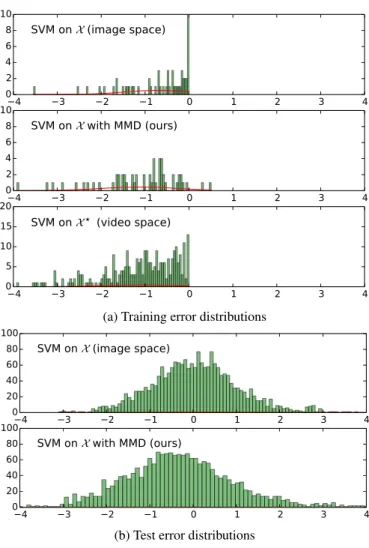
in-(a) Training error distributions
(b) Test error distributions
Figure 2: Visualization of the error distributions of three classifiers in the experiment with Image+Video dataset. For
a binary problem of differentiating akayakingaction from
others, we compare pd when training SVM on original
data spaceX,pdwith KL(pd⋆||pd)when training our proposed
SVM MMD on data fromX andX⋆, andpd⋆when training
SVM on privileged data spaceX⋆. In this case, our
pro-posed method successfully utilizes privileged information:
the peak of train (2a: middle) and test (2b: middle)
distri-butionspdwith KL(pd⋆||pd)are shifted to theleftcomparing to
pd. Train and test cases ofpd⋆ are the same as we use all
available datain the other datasetas privileged information.
stance based on its privileged data (requires one-to-one
cor-respondence). Instead in Eq. (2), we match the distribution
of errors in privileged and original spaces (correspondence-free setting). Our intuition is that making errors on an in-stance basis is unavoidable, but we will make better deci-sions at a large scale by comparing error distributions.
To compute the KL divergence, we require a
paramet-ric assumption on the distributionpd⋆ as well aspd. If we
assume thatX⋆ is of much better quality thanX as in for
example [35,28], the distribution of the slack variables on
privileged spaced⋆
will have a mean value in the negative region (for a correct prediction with a high confidence, the
functional margin y⋆
i hw⋆,x⋆iiwill be large and therefore
the slack variable will be negative). Whereas, the
distri-bution of the slack variables in the original space,pd, will
have a mean value around zero and tails that accounts for correctly (left tail) classified samples at negative region and incorrectly (right tail) classified samples at positive region. Please, refer to our visualization of the distribution over the
deviation values in Figure2.
In the simplest case, we could model thepddistribution
with the Gaussian exponential family, pd = N(d|µd, σ2
d).
With this assumption, minimizing KL(pd⋆||pd)reduces to
matchingthe first and secondmomentsof the two
distribu-tions, which are the mean and the variance.
4.2. Maximum Mean Discrepancy
We can go beyond the Gaussian assumption and match skewness, kurtosis (third and fourth moments) or even higher order moments. In a more general case, to avoid a parametric assumption on the distance estimate between distributions, we propose to use the Maximum Mean
Dis-crepancy (MMD) criterion [12], a non-parametric distance
estimate. Denote byHa Reproducing Kernel Hilbert Space
with kernelkdefined onX. In this case one can show [12]
that wheneverkis characteristic (or universal), the map
µ:p→µ[p] :=Ed∼pd[k(d,·)]
with associated distance
MMD(pd⋆, pd) :=kµ[pd⋆]−µ[pd]k2 (3)
characterizes a distribution uniquely. Examples of
char-acteristic kernels [31] are Gaussian RBF, Laplacian and
B2n+1-splines. With a this choice of kernel functions, the
MMD criterion matches infinitely many moments in the Re-producing Kernel Hilbert Space (RKHS). The mean and variance matching described in the previous section is a
spe-cial case when we use a polynomial kernel with degree2.
We use a biased estimate of MMD as follows: \ MMD= 1 N2 N X i N X i′ k(di, di′)− 2 N N⋆ N X i N⋆ X j k(di, d⋆ j)+ + 1 N⋆,2 N⋆ X j N⋆ X j′ k(d⋆ j, d ⋆ j′). (4)
The above quantity is then used as a plug-in estimator for
non-parametric KL(pd⋆||pd)in (2). Please refer to Alg. 1
for the summary of our proposed method.
RemarkUsing non universal kernels such as a polyno-mial kernel will only give necessary but not sufficient con-ditions for distribution matching. Hence we use RBF kernel
Algorithm 1Matching Error distributions onX⋆andX Inputoriginal data(X, Y), privileged data(X⋆, Y⋆),
assumef(x) :=hw,xiandf⋆(x⋆) :=hw⋆,x⋆i w⋆←solve||w⋆||2+ hingeloss(w⋆|X⋆, Y⋆) D∗={1−y⋆ i hw⋆,x⋆ii}N ⋆ i=1(errors onX⋆) w←solve||w||2+MMDloss (\ D⋆, D(w)|X, Y) s.t.D(w) ={1−yihw,xii}N i=1(errors onX) Returnw
in the MMD criterion, while maintaining a linear classifier form in the proposed method. Computing MMD criterion
in Eq. (4) costsO((N+N⋆)2)time [12], this is true for any
kernel. We plan to explore advancements in fast two-sample
test with cost that is linear in number of samples (e.g. [5]).
5. Experiments
We study the task of object as well as action recognition in images with three possible types of privileged
informa-tion available at training time:clip art illustrations,videos,
and3D models. The classification task is the same in both
modalities, so that the privileged data is informative about the objects/actions that we are primarily interested to recog-nize using the image modality.
Datasets. We use four publicly available datasets to test the performance of our cross-modal/dataset scenario:
the INTERACT1 dataset [1] with clip art illustrations
col-lected in addition to images that capture the interaction
be-tween people, the UCF1012 action recognition dataset of
videos [30], and the CrossLink3 dataset [16] of
3DWare-house4 models accompanied by the action and object
im-ages from the ImageNet dataset5[26].
Methods. We compare our SVM MMD model (SVM MMD) with a standard object classification baseline such
as SVM classifier trained on the image space X (SVM
Images). To put our method into perspective of do-main adaptation and provided that the feature
dimension-ality is the same across modalities X and X⋆
, we
com-pare the proposedSVM MMDwith theinstance-transfer
ap-proach that shares the data samples between the two modal-ities, i.e. SVM trained on union of image and privileged
data (SVM Combined); and the model-transfer method
that relies on parameter transfer from privileged (source)
to image (target) space, such as adaptive SVM [19, 39]
(SVM Adaptive). For a given solution of the source
task, wsource, and training data of the target task, SVM
Adaptivesolves the following optimization problem: 1 https://computing.ece.vt.edu/˜santol/projects/zsl_ via_visual_abstraction/interact/index.html 2http://crcv.ucf.edu/data/UCF101.php 3http://geometry.cs.ucl.ac.uk/projects/2015/crosslink 4https://3dwarehouse.sketchup.com/?hl=en 5http://www.image-net.org minimize w kw−wsourcek2+ C N N X j=1 ξj (5)
s.t. 1−yjhw,xji ≤ξj, ξj ≥0 for all 1≤j≤N.
To train a classifier on image data, we solve (5) using as
wsource the weight vector obtained from training using the
privileged data. From the perspective of domain adaptation, SVM Adaptivetransfers the information by introducing
thebias into the regularizationterm of SVM, whereas the
proposed MMD model introduces thebias into the lossterm
of the SVM. We also provide a reference comparison with
the SVM+ baseline (SVM+) [35] that relies on the
one-to-one correspondence between samples in the original and
privileged spaces if applicable (Section5.1).
Model selection. We perform a cross-validation model selection approach for choosing the regularization trade-off parameter(s) for each of the methods. In all our
ex-periments, we select C over 5 hyper-parameter values
{100,101. . . ,104} using5×3 fold cross-validation. We
setC⋆ to be 100everywhere except in SVM+. We use a
Gaussian RBF kernel for the MMD term with a fixed kernel
width of 10.0. From what we observed, theSVM+baseline
requires a broad range to infer its two hyper-parameters,C
andC⋆
, so we perform5×3fold joint cross-validation over
the range{10−4,10−3, . . . ,104}.
Evaluation metric. To evaluate the performance of the methods, we use the classification accuracy. We repeat each
experiment 20 times using different random splits of the
data into train and test sets and report mean and standard error across repeats.
5.1. Learning from the mistakes in abstract images
The INTERACT dataset contains60fine-grained classes
that capture a variety of interactions between a pair of
peo-ple, e.g., running after,running to,arguing with. Each of
the interaction is represented as a set of real images and
a set of clip art illustrations (on average, 50 images and
50 illustrations per class). The dataset has two settings:
category-level, in which images and illustrations are
col-lected independently given the category class, and
instance-levelwhere 2-3 illustrations are collected for a given image. Here, we detail the experimental results of the category-level setting, and the supplementary material contains the full table of results of the instance-level setting.
For each interaction class, we train a binary classifier to distinguish this interaction (positive class) against the
re-maining59interactions (negative class). To train a
classi-fier, we randomly sample25positive vs25negative images,
and for testing we use the remaining positive images bal-anced with the negative samples. For those methods that
use privileged data (for training only), we take 50clip art
illustrations as positive samples (all available per class) and balance them with the clip art images from the negative
(a) Image + Clip art (b) Image + 3D model (c) Image+Video (spatial+motion) (d) Image+Video (spatial) (e) Image+Video (motion)
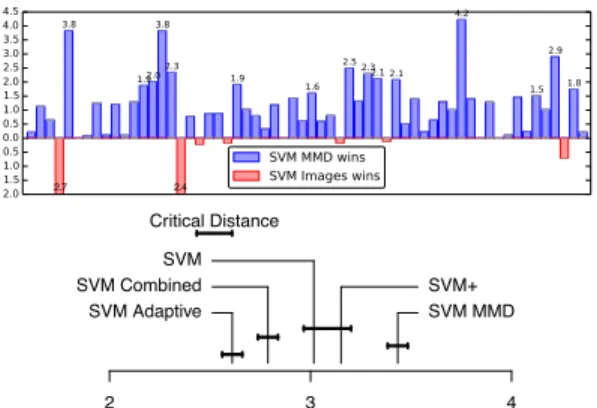
Figure 3: Learningimageclassifiers from the mistakes of
classifiers trained onotherdatasets:clip arts(3a),3D
mod-els(3b), andvideos(3c–3e) datasets. Pairwise comparison
of the proposed SVM MMD and the baseline method (SVM trained on images). The height of the bar corresponds to the relative accuracy improvement over the baselines for each
of the60one-versus-rest (Image + Clip art),36
one-versus-one (Image + 3D model), and15one-versus-rest (Image +
Video) problems. The full accuracy results are presented in
Tables1,2, and in the supplementary material.
● 2 3 4 SVM MMD SVM+ SVM Adaptive SVM Combined SVM Critical Distance
(a) Image + Clip art
● 2 3 4 SVM MMD SVM SVM Adaptive SVM Combined Critical Distance (b) Image + 3D model ● 1 2 3 4 5 6 7 SVM MMD (motion) SVM MMD (spatial) SVM MMD (spatial+motion) SVM (images) SVM Adaptive (motion) SVM Combined (motion) SVM Adaptive (spatial) SVM Combined (spatial) (c) Image + Video
Figure 4: Statistical summary of results based on
Demˇsar [6]. Average rank of the methods (x axis) is
com-puted based on accuracy (the higher the better). A critical distance measures significant differences between methods based on their ranks. We link two methods with a solid line
if they are not statistically different (p-value>5%).
classes. In this experiment, to train SVM+, we randomly pair images and illustrations of the same class label to define
the constraints in Eq. (1b). In the instance-level setting (in
the supplementary), we use one corresponding illustration per image. We noticed that within an action category, the variability of clip art illustrations is moderate, and SVM+ performs similarly in category and instance-level settings.
In this dataset, real images and clip art illustrations are
represented using765dimensional features that capture
hu-man poses, expressions, relation and appearance and are provided with the dataset. We use the features computed for Person A, who is performing the action with respect to Person B. In this case the privileged modality and the real images are expressed using the same feature representation, which makes it a perfect testbed to compare our proposed model with all baselines.
Results. The full result of this experiment is presented
in Table 1 and the summary in terms of a pairwise
com-parison between the proposed SVM MMD and the standard
SVM is in Figure 3a. We analyzed our experimental
re-sults on the INTERACT dataset using the multiple dataset
statistical comparison method of [6] in Figure4a. There is
statistical evidence that SVM MMD performs best among the five methods. SVM+ performs better than SVM and SVM Combined in terms of ranking, however there is not enough evidence to support that the differences are signifi-cant. This conclusion holds true also for the instance-level
setting (summarized in Figure 5). Advantageous
perfor-mance of SVM MMD shows that learning from the mis-takes of clip art classifiers help. We credit the significant improvement of SVM MMD over other methods to the prin-cipled idea of making the right decision at a larger scale by comparing error distributions rather than focusing on error
in example-by-example basis. From theaverage rank
per-spective, SVM Combined and SVM Adaptive do not lead to an improved performance w.r.t. SVM Images.
Look-ing closer at Table1, there are cases when SVM Combined
improves significantly (sitting with) and SVM Adaptive im-proves by a large margin (elbowing) but they are followed
by large performance dips in cases such as looking away
from(SVM Combined) andtalking with(SVM Adaptive).
In contrast, the drop in SVM MMD is only moderate at
worst (actionwaving at).
5.2. Learning from the mistakes in videos
In this experiment, we cross video data from the UCF101 dataset with image data from the ImageNet dataset to ad-dress the task of action recognition in images. Both datasets
intersect at sport activities, so we focus on the following15
actions: archery,basketball,biking,bowling,cricket shot,
golf swing,horse riding,kayaking,pole vault,rafting,
row-ing,skateboard,skiing,surfingandtennis swing. We
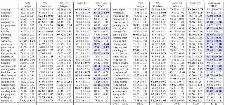
SVM SVM SVM[39] SVM+[35] SVM(ours)
Images Combined Adaptive MMD
carrying 97.21±0.33 94.50±0.55 96.36±0.46 97.64±0.39 97.43±0.46 catching 83.75±1.15 84.20±1.15 83.41±1.18 84.20±1.10 85.11±1.10 pushing 80.08±1.14 82.74±0.90 81.37±1.17 80.89±0.93 80.24±1.15 pulling 63.79±0.89 67.18±1.55 64.60±1.42 62.82±1.11 63.79±1.30 reaching for 66.42±0.86 68.58±1.02 67.17±1.18 66.50±1.36 68.50±1.04 jumping over 90.10±0.95 93.17±0.55 93.46±0.84 90.77±0.88 89.81±0.86 hitting 83.89±1.39 83.70±1.28 84.07±1.24 83.43±1.29 84.26±1.11 kicking 89.67±1.05 92.17±0.68 91.08±0.81 90.75±0.91 90.75±0.79 elbowing 82.39±1.00 84.43±1.19 86.82±0.87 83.86±1.15 83.86±0.95 tripping 86.36±0.79 84.39±0.96 85.23±1.05 86.82±0.61 87.88±0.74 waving at 71.20±1.29 67.72±1.50 68.04±1.43 70.33±1.05 69.67±1.11 pointing at 77.33±1.34 74.22±1.47 73.79±1.62 77.16±1.38 78.79±1.23 point. aw. fr. 66.50±1.67 66.00±1.74 63.62±1.76 67.00±1.39 67.88±1.72 looking at 67.42±1.37 68.95±1.75 66.13±1.28 67.50±1.71 66.69±1.49 looking aw. fr. 73.91±1.61 67.66±0.91 70.55±1.25 73.12±1.22 75.23±1.29 laughing at 72.34±0.98 74.22±1.28 71.95±1.05 73.20±0.95 74.14±1.16 laughing with 82.29±0.90 81.88±1.10 79.90±1.32 80.21±1.12 80.83±1.05 hugging 87.89±0.96 87.66±1.16 88.36±0.96 88.44±0.75 87.42±0.91 wrestling with 88.75±0.87 85.80±0.98 87.39±0.81 89.66±0.87 90.11±0.95 dancing with 84.34±0.82 81.10±1.32 82.72±1.09 83.82±1.04 84.56±0.82 hold. hands w. 85.48±0.75 83.87±0.99 84.60±0.79 86.13±0.71 86.05±0.71 shak. hands w. 94.74±0.84 91.12±0.69 92.76±0.69 95.69±0.51 94.91±0.67 talking with 82.06±0.94 79.49±1.39 76.54±1.06 81.62±1.40 82.21±1.17 arguing with 83.62±1.02 83.97±0.80 85.17±0.88 83.88±1.13 83.28±0.85 walking with 91.93±0.63 90.00±0.89 89.43±1.06 93.30±0.57 93.41±0.58 running with 89.67±0.89 87.67±1.22 89.58±1.00 89.67±0.88 89.33±0.97 crawling with 79.76±1.47 82.38±0.85 80.12±1.23 81.19±1.46 82.02±1.24 jumping with 82.88±0.96 83.46±1.61 81.73±1.56 81.92±1.12 83.08±0.83 walking to 78.75±1.26 79.73±0.81 77.68±1.15 79.64±1.04 79.20±1.16 running to 78.12±1.10 77.81±0.79 77.42±0.97 77.81±1.14 78.05±1.20 SVM SVM SVM[39] SVM+[35] SVM(ours)
Images Combined Adaptive MMD
crawling to 82.14±0.79 79.02±1.16 79.55±1.19 83.39±0.78 83.12±0.76 jumping to 78.88±1.15 80.95±0.98 79.14±1.06 80.00±1.09 80.26±1.26 walking aw. fr. 78.87±1.12 78.15±0.80 76.69±1.24 78.47±0.86 79.03±0.95 running aw. fr. 84.29±1.36 83.04±0.77 84.64±0.91 83.12±1.21 84.11±1.06 crawling aw. fr. 78.64±1.48 80.23±1.36 76.59±1.84 77.73±1.44 81.82±1.60 jumping aw. fr. 83.98±0.94 83.59±0.87 82.66±1.04 83.44±1.00 83.75±0.79 walking after 84.20±0.98 81.40±0.98 82.80±0.88 85.50±1.11 87.10±0.78 running after 82.95±1.03 81.44±1.02 84.17±0.98 83.79±0.96 83.86±0.71 crawling after 86.67±0.91 84.88±1.01 83.57±1.04 86.19±1.06 86.67±1.04 jumping after 81.42±0.74 80.83±0.78 79.00±0.90 81.08±0.85 82.17±0.85 walking past 80.15±1.01 80.74±0.81 78.53±1.43 80.51±0.91 81.76±0.75 running past 76.09±1.40 77.27±1.18 75.23±1.41 77.58±1.45 78.12±1.10 crawling past 78.10±1.79 78.45±1.29 77.62±1.17 77.26±1.65 78.69±1.58 jumping past 77.41±1.31 73.15±1.71 74.54±1.70 76.67±1.84 77.41±1.45 stand. next to 84.35±0.61 84.89±0.71 81.63±0.95 83.80±0.78 83.70±0.82 sitting next to 85.70±1.03 84.69±0.85 83.52±0.83 84.77±1.06 86.33±0.90 lying next to 73.45±1.32 73.88±0.89 74.31±1.16 73.36±1.27 74.57±1.10 crouch. next to 80.31±1.56 80.16±1.00 78.59±1.37 80.78±1.55 80.16±1.37 stand. in fr. of 71.79±1.46 67.14±1.06 69.07±1.28 72.07±1.34 73.14±1.18 sitting in fr. of 78.56±0.95 79.70±1.08 79.09±0.96 78.48±1.12 79.85±1.02 lying in fr. of 81.98±1.01 81.12±0.92 83.10±0.86 82.76±0.98 81.47±1.16 crouch. in fr. of 87.27±0.91 87.05±1.25 86.93±1.20 86.70±0.82 88.75±0.78 standing behind 71.03±1.30 70.52±1.55 71.98±1.28 68.79±1.47 71.64±1.39 sitting behind 87.98±0.79 89.19±0.62 88.39±0.79 88.63±0.84 88.95±0.81 lying behind 80.68±1.17 83.11±1.09 82.27±0.99 81.14±1.08 82.42±0.95 crouch. behind 76.30±1.14 76.30±1.11 75.09±1.08 76.11±0.84 76.94±1.07 standing with 78.15±1.39 78.79±1.29 74.35±1.48 79.03±1.07 80.65±0.96 sitting with 81.90±1.21 85.83±1.23 84.29±1.17 82.50±1.01 83.33±1.06 lying with 70.50±1.13 70.92±1.22 68.25±1.24 71.58±1.02 71.33±1.14 crouch. with 79.78±1.34 81.09±1.01 80.33±0.95 80.00±1.08 79.89±1.12 avg. acc. 80.77 80.45 79.95 80.90 81.49 Table 1: Learning image classifiers with the mistakes of clip art classifiers (category-level setting). For instance-level setting,
please refer to the supplementary material. The best result is highlighted inboldfacewith an extra blue for our SVM MMD.
spatial+motion spatial motion
SVM SVM(ours) SVM SVM [39] SVM (ours) SVM SVM [39] SVM (ours) Images MMD Combined Adaptive MMD Combined Adaptive MMD Archery 83.87±0.50 85.44±0.30 83.48±0.24 82.81±0.36 85.69±0.27 79.75±0.70 73.47±0.61 85.67±0.28 Basketball 91.95±0.33 91.89±0.27 90.04±0.35 87.60±0.48 92.16±0.26 89.82±0.42 82.25±0.49 92.30±0.30 Biking 90.71±0.24 91.26±0.32 89.93±0.33 88.49±0.31 91.44±0.20 86.87±0.52 79.54±0.54 91.45±0.21 Bowling 94.66±0.29 94.18±0.38 93.24±0.32 90.09±0.47 94.27±0.34 90.61±0.59 85.72±0.50 94.59±0.34 CricketShot 84.96±0.28 85.29±0.66 83.77±0.24 82.92±0.33 85.90±0.22 82.44±0.43 78.97±0.54 85.84±0.22 GolfSwing 82.17±0.49 83.06±0.31 81.13±0.41 80.03±0.32 83.00±0.30 80.51±0.34 72.76±0.53 83.23±0.29 HorseRiding 90.39±0.15 90.60±0.18 90.18±0.24 89.05±0.32 90.63±0.20 87.37±0.55 79.56±0.43 90.49±0.25 Kayaking 83.14±0.45 85.45±0.19 82.27±0.37 81.97±0.46 85.35±0.23 81.16±0.47 75.28±0.50 85.37±0.26 PoleVault 87.86±0.44 88.20±0.41 84.41±0.33 83.97±0.37 88.11±0.37 83.53±0.66 77.34±0.35 88.54±0.39 Rafting 87.55±0.29 87.97±0.27 87.54±0.27 86.35±0.28 88.03±0.16 85.40±0.39 82.29±0.38 88.33±0.21 Rowing 87.80±0.46 87.71±0.36 89.49±0.18 88.32±0.23 87.84±0.35 85.05±0.52 80.13±0.36 87.91±0.31 SkateBoarding 81.13±0.54 82.39±0.42 81.46±0.43 79.83±0.48 82.37±0.36 77.48±0.67 72.32±0.50 82.70±0.40 Skiing 90.24±0.45 90.61±0.45 90.24±0.24 88.49±0.38 90.59±0.31 86.93±0.52 79.62±0.39 91.18±0.25 Surfing 88.52±0.39 88.85±0.28 88.64±0.26 87.76±0.32 88.65±0.35 86.34±0.26 82.87±0.46 89.15±0.21 TennisSwing 83.35±0.47 83.59±0.42 82.78±0.32 81.62±0.31 83.69±0.36 79.49±0.64 72.58±0.67 83.82±0.41 avg. acc. 87.22 87.77 86.57 85.29 87.85 84.18 78.31 88.04
Table 2: Learning image classifiers with the mistakes of video classifiers. Video data contain complementary information from still frames (spatial) and motion between frames (motion). The best result, for each of the video information (spatial,
motion, and spatial+motion), is highlighted inboldfaceand an extra blue for our SVM MMD.
dataset to these action classes to form the image data
modal-ity. On average, each action class has1000images and100
videos to train/test the models. Similarly to our previous
experiment, we form 15 one-vs-rest binary classification
tasks by randomly sampling28 vs28 images for training
and1000vs1000images to test the methods (or as much
as the class size allows). For those methods that use priv-ileged data (for training only), we take all videos from the positive class and balance them with the same amount ran-domly sampled from the negative classes. As our image
representation, we use4096dimensional features extracted
from the fc7 activation layer in CaffeNet [17] fine-tuned on
ImageNet VOC2012 [26]. As our video representation, we
extract spatial and temporal representations from the Caffe models fine-tuned on ImageNet VOC2012 (the same as im-age data) and on optical flow of the UCF101 dataset as
pro-vided in [11]. This video representation allows us to study
the effects of three types of privileged data in this scenario:
the spatial signal alone (4096dimensional), the motion
sig-nal alone (4096dimensional), and the spatial+motion
sig-nals combined (8192dimensional). The first two types, as
2.7 2.4 ● 2 3 4 SVM MMD SVM+ SVM Adaptive SVM Combined SVM Critical Distance
Figure 5: Learning image classifiers with the mistakes of clip art classifiers (instance-level setting). The full results are in the supplementary material.
used by the two domain adaptation baselines (SVM Adap-tive and SVM Combined), whereas the spatial+motion in-formation can not be used unless projection matrices are learned. Our SVM MMD does not depend on the dimen-sionality of the privileged data space.
Results. The results of this experiment are presented in
Table 2, the summary in terms of a pairwise comparison
between the proposed SVM MMD and the standard SVM
is depicted in Figure 3c–3e, and statistical comparison of
all methods is reported in Figure4c. Overall, SVM MMD
clearly improves over SVM Images in all settings of video information: spatial, motion, and spatial+motion.
Specif-ically, in all cases but one, bowling, we can see positive
improvements when using video modality as privileged in-formation. The largest improvement appears when SVM MMD learns only from the mistakes of video classifiers
withmotionfeatures. This can be credited to the
comple-mentary view of motion features w.r.t. the original image space and a good motion feature representation (deep fea-tures fine-tuned on optical flow of the UCF101 dataset).
5.3. Learning from the mistakes in 3D models
In contrast to our main task of object/action recognition in images, the CrossLink dataset was primarily designed to improve the performance of the 3D retrieval by leveraging images from the Bing search. We explore the setting where 3D models from the 3DWarehouse collection are used as privileged data to the images from the more complex
Im-ageNet dataset. We collect 3D models by crawling the
3DWarehouse as described in [16], and manually checked
all the models. Each 3D model is retrieved as a collection
of36views of the object taken against no background. We
use ImageNet synsets as our main image data. We focus on
the following9 classes: airplane,backpack,bicycle,boat,
car,chair,couch,helicopter,laptop. Each object class has
1300images on average and903D models, ranging from15
to153instances per class. As our image representation, we
use4096dimensional deep features from the fc7 activation
layer in CaffeNet fine-tuned on ImageNet VOC2012. As
3D model representation, we extract the same4096
dimen-sional deep features from each of the views, and consider
them as36data samples in the privileged space. For each
pair of the9classes (36in total) we train a one-vs-one
bi-nary classifier using50images (class balanced) for training
and 2000images (class balanced) for testing the models.
For those methods that use privileged data, we balance25
vs25instances of 3D models randomly sampled from the
positive and negative classes.
Results. The full result of this experiment is presented in Table 1 of the supplementary material and the summary in terms of a pairwise comparison between the proposed
SVM MMD and the standard SVM is in Figure3b. Overall,
SVM MMD improves over SVM Images (also supported by
statistical summary in Figure4b), but the actual
improve-ment is minor. We credit this to the fact, that this recogni-tion problem is rather simple, and the SVM Images baseline
alone has achieved an average accuracy of95.78%.
6. Conclusion and future work
A fool learns from his mistakes, but a truly wise man learns from the mistakes of others.
Otto von Bismarck Learning with privileged information (LUPI) aims to
ex-ploit extra information that is available foreach instanceat
training time. A typical assumption made is that these
ex-tra data are useful to discriminate betweeneasyanddifficult
instances. We generalize this idea by describing a model
that uses a divergence between distribution ofour own
er-rorsand ofothers’ errorsas the loss function. Our approach
can handle setting with no strict one-to-one correspondence between privileged and original data. We have shown the usefulness of this correspondence-free LUPI in the setting of cross-dataset learning of image classifiers. Our results reveal that learning image classifiers with the mistakes of clip art classifiers, or 3D classifiers, or video classifiers can be more accurate than learning using images only.
We seek to generalize our findings on correspondence-free LUPI for regression and multiple privileged informa-tion settings. We also aim to unify the LUPI setting and the setting where the extra attributes are available at test
time but not at training time [18] under our framework of
divergence minimization between the classifier errors in the privileged and original spaces. Finally, in the direction of deep model compression or distillation, we will assess the benefits of error matching as an alternative to matching the output class-probabilities commonly used in the literature.
Acknowledgment
We gratefully acknowledge NVIDIA for GPU donation and Amazon for AWS Cloud Credits.
References
[1] S. Antol, C. L. Zitnick, and D. Parikh. Zero-shot learning via visual abstraction. InECCV, 2014.3,5
[2] J. Ba and R. Caruana. Do deep nets really need to be deep? InNIPS, 2014.2
[3] M. Belkin, P. Niyogi, and V. Sindhwani. Manifold regular-ization: A geometric framework for learning from labeled and unlabeled examples.JMLR, pages 2399–2434, 2006.3
[4] J. Chen, X. Liu, and S. Lyu. Boosting with side information. InACCV, 2013.3
[5] K. Chwialkowski et al. Fast two-sample testing with analytic representations of probability measures.NIPS, 2015.5
[6] J. Demˇsar. Statistical comparisons of classifiers over multi-ple data sets.JMLR, pages 1–30, 2006.6
[7] L. Duan, Y. Xu, W. Li, L. Chen, D. W. K. Wong, T. Y. Wong, and J. Liu. Incorporating privileged genetic info. for fundus image based glaucoma detection. InMICCAI, 2014.1
[8] J. Feyereisl and U. Aickelin. Privileged information for data clustering.Information Sciences, pages 4–23, 2012.1
[9] J. Feyereisl, S. Kwak, J. Son, and B. Han. Object localiza-tion based on structural svm using privileged informalocaliza-tion. In
NIPS, 2014.1
[10] S. Fouad, P. Tino, S. Raychaudhury, and P. Schneider. In-corporating privileged information through metric learning.
T-NNLS, 2013.1
[11] G. Gkioxari and J. Malik. Finding action tubes. InCVPR, 2015.7
[12] A. Gretton, K. Borgwardt, M. Rasch, B. Sch¨olkopf, and A. Smola. A kernel method for the two-sample-prob. In
NIPS, 2006.2,4,5
[13] S. Gupta, J. Hoffman, and J. Malik. Cross modal distillation for supervision transfer. InCVPR, 2016.2
[14] D. Hern´andez-Lobato, V. Sharmanska, K. Kersting, C. H. Lampert, and N. Quadrianto. Mind the nuisance: Gaussian process classification using privileged noise. InNIPS, 2014.
1,2,3
[15] G. E. Hinton, O. Vinyals, and J. Dean. Distilling the knowl-edge in a neural network.arXiv preprint arXiv:1503.02531, 2015.2
[16] M. Hueting, M. Ovsjanikov, and N. Mitra. Crosslink: Joint understanding of image and 3D model collections through shape and camera pose variations. SIGGRAPH Asia, 2015.
5,8
[17] Y. Jia, E. Shelhamer, J. Donahue, S. Karayev, J. Long, R. Gir-shick, S. Guadarrama, and T. Darrell. Caffe: Convolu-tional architecture for fast feature embedding.arXiv preprint arXiv:1408.5093, 2014.7
[18] S. Khamis and C. H. Lampert. CoConut: Co-classification with output space regularization. InBMVC, 2014.8
[19] W. Kienzle and K. Chellapilla. Personalized handwriting recognition via biased regularization. InICML, 2006.5
[20] M. Lapin, M. Hein, and B. Schiele. Learning using privi-leged information: SVM+ and weighted SVM. Neural Net-works, pages 95–108, 2014.1
[21] W. Li, L. Duan, D. Xu, and I. W. Tsang. Learning with augmented features for supervised and semi-supervised het-erogeneous domain adaptation. T-PAMI, pages 1134–1148, 2014.2
[22] D. Lopez-Paz, L. Bottou, B. Sch¨olkopf, and V. Vapnik. Uni-fying distillation and privileged information. InICLR, 2016.
2
[23] S. J. Pan, I. W. Tsang, J. T. Kwok, and Q. Yang. Domain adaptation via transfer component analysis. InIJCAI, 2009.
2
[24] D. Pechyony and V. Vapnik. Fast optimization algorithms for solving SVM+. InStat. Learning and Data Science, 2011.1
[25] N. Quadrianto, J. Petterson, and A. Smola. Distribution matching for transduction. InNIPS, 2009.2
[26] O. Russakovsky, J. Deng, H. Su, J. Krause, S. Satheesh, S. Ma, Z. Huang, A. Karpathy, A. Khosla, M. Bernstein, A. C. Berg, and L. Fei-Fei. ImageNet Large Scale Visual Recognition Challenge.IJCV, pages 1–42, 2015.5,7
[27] V. Sharmanska, D. Lobato, J. M. Hern´andez-Lobato, and N. Quadrianto. Ambiguity helps: Classification with disagreements in crowdsourced annotations. InCVPR, 2016.1
[28] V. Sharmanska, N. Quadrianto, and C. H. Lampert. Learning to rank using privileged information. InICCV, 2013.1,2,3,
4
[29] V. Sindhwani and D. S. Rosenberg. An rkhs for multi-view learning and manifold co-regularization. InICML, 2008.3
[30] K. Soomro, A. R. Zamir, and M. Shah. UCF101: A dataset of 101 human actions classes from videos in the wild.arXiv preprint arXiv:1212.0402, 2012.5
[31] B. K. Sriperumbudur, K. Fukumizu, and G. R. G. Lanckriet. Universality, characteristic kernels and RKHS embedding of measures.JMLR, pages 2389–2410, 2011.4
[32] T. Tommasi and T. Tuytelaars. A testbed for cross-dataset analysis. InECCV Workshop, 2014.2
[33] E. Tzeng, J. Hoffman, T. Darrell, and K. Saenko. Simultane-ous deep transfer across domains and tasks. InICCV, 2015.
2
[34] V. Vapnik and R. Izmailov. Learning using privileged infor-mation: Similarity control and knowledge transfer. JMLR, pages 2023–2049, 2015. 1
[35] V. Vapnik and A. Vashist. A new learning paradigm: Learn-ing usLearn-ing privileged information. Neural Networks, pages 544–557, 2009.1,2,3,4,5,7
[36] Z. Wang, X. Wang, and Q. Ji. Learning with hidden infor-mation. InICPR, 2014.3
[37] D. X. Wen Li, Li Niu. Exploiting privileged information from web data for image categorization. InECCV, 2014.1
[38] H. Yang and I. Patras. Privileged information-based condi-tional regression forest for facial feature detection. In Auto-matic Face and Gesture Recognition (FG), 2013.1
[39] J. Yang, R. Yan, and A. G. Hauptmann. Cross-domain video concept detection using adaptive SVMs. InACM MM, 2007.
5,7
[40] X. Zhang, F. X. Yu, S.-F. Chang, and S. Wang. Deep transfer network: Unsupervised domain adaptation. arXiv preprint arXiv:1503.00591, 2015.2
![Figure 4: Statistical summary of results based on Demˇsar [6]. Average rank of the methods (x axis) is com-puted based on accuracy (the higher the better)](https://thumb-us.123doks.com/thumbv2/123dok_us/1453380.2694506/6.918.80.424.700.966/figure-statistical-summary-results-demˇsar-average-methods-accuracy.webp)