MATHICSE
Mathematics Institute of Computational Science and Engineering
School of Basic Sciences - Section of Mathematics
Address:
EPFL - SB - MATHICSE (Bâtiment MA) Station 8 - CH-1015 - Lausanne - Switzerland
http://mathicse.epfl.ch
Phone: +41 21 69 37648 Fax: +41 21 69 32545
Discrete least squares polynomial
approximation with random
evaluations – application to
parametric and stochastic
elliptic PDES
Abdellah Chkifa, Albert Cohen, Giovanni Migliorati, Fabio Nobile, Raul Tempone
MATHICSE Technical Report
Nr. 35.2013
Mod´elisation Math´ematique et Analyse Num´erique
DISCRETE LEAST SQUARES POLYNOMIAL APPROXIMATION
WITH RANDOM EVALUATIONS - APPLICATION TO PARAMETRIC
AND STOCHASTIC ELLIPTIC PDES
Abdellah Chkifa
1, Albert Cohen
2, Giovanni Migliorati
3, Fabio
Nobile
4and Raul Tempone
5Abstract. Motivated by the numerical treatment of parametric and stochastic PDEs, we analyze the least-squares method for polynomial approximation of multivariate func-tions based on random sampling according to a given probability measure. Recent work has shown that in the univariate case, the least-squares method is quasi-optimal in expec-tation in [8] and in probability in [20], under suitable conditions that relate the number of samples with respect to the dimension of the polynomial space. Here “quasi-optimal” means that the accuracy of the least-squares approximation is comparable with that of the best approximation in the given polynomial space. In this paper, we discuss the quasi-optimality of the polynomial least-squares method in arbitrary dimension. Our analysis applies to any arbitrary multivariate polynomial space (including tensor product, total degree or hyperbolic crosses), under the minimal requirement that its associated index set is downward closed. The optimality criterion only involves the relation between the number of samples and the dimension of the polynomial space, independently of the anisotropic shape and of the number of variables. We extend our results to the approx-imation of Hilbert space-valued functions in order to apply them to the approxapprox-imation of parametric and stochastic elliptic PDEs. As a particular case, we discuss “inclusion type” elliptic PDE models, and derive an exponential convergence estimate for the least-squares method. Numerical results confirm our estimate, yet pointing out a gap between the condition necessary to achieve optimality in the theory, and the condition that in practice yields the optimal convergence rate.
1991 Mathematics Subject Classification. 41A10, 41A25, 65N35, 65N12, 65N15, 35J25.
.
Keywords and phrases:approximation theory, polynomial approximation, least squares, parametric and stochas-tic PDEs, high-dimensional approximation.
1 UPMC Univ Paris 06, UMR 7598, Laboratoire Jacques-Louis Lions, F-75005, Paris, France. email:
2 UPMC Univ Paris 06, UMR 7598, Laboratoire Jacques-Louis Lions, F-75005, Paris, France. email:
3 MATHICSE-CSQI, ´Ecole Polytechnique F´ed´erale de Lausanne, Lausanne CH-1015, Switzerland and
MOX-Department of Mathematics, Politecnico di Milano, Milano 20133, Italy. email: [email protected]
4 MATHICSE-CSQI, ´Ecole Polytechnique F´ed´erale de Lausanne, Lausanne CH-1015, Switzerland and
MOX-Department of Mathematics, Politecnico di Milano, Milano 20133, Italy. email: [email protected]
5Applied Mathematics and Computational Sciences, and SRI Center for Uncertainty Quantification in
Compu-tational Science and Engineering, KAUST, Thuwal 23955-6900, Saudi Arabia. email: [email protected]
1.
Introduction
In recent years, various strategies have been proposed for the numerical treatment of parametric and stochastic partial differential equations
D(u, y) = 0, (1)
whereu7→ D(u, y) is a partial differential operator depending on ad-dimensional parameter vector
y:= (y1, . . . , yd)∈Γ⊂Rd. (2) Depending on the application, the parameter vector may be deterministic or stochastic. In the latter case y is a random variable distributed over Γ according to a probability measureρ. We denote by (Γ,Σ, ρ) the corresponding probability space, where Σ is the Borelσ-algebra. In certain applications one has to deal with a countable number of parametersy= (yj)j≥1which means that
d= +∞.
Assuming well-posedness of the problem in some Banach spaceX, the solution map
y7→u(y), (3)
is defined from the parameter domain Γ to the solution space X. In both deterministic and stochastic settings, the main challenge is to approximate the functiony7→u(y) with a reasonable cost. In the first setting, one typically searches for approximations that are uniformly accurate over the parameter space Γ, which amounts in measuring the error in L∞(Γ, X). In the second setting, one is typically interested in approximations that are accurate in a probabilistic sense, such as in the least-squares sense which amounts in measuring the error inL2(Γ, X, ρ).
Polynomial approximation methods of the solution map have been studied for various types of operators Dcorresponding to various PDEs. In such methods, the solution map is approximated by polynomial maps of the form
uΛ(y) =X
ν∈Λ
uνyν, (4)
where Λ⊂ F is a finite set of (multi-)indices. The set of multi-indicesF coincides withNd
0 where N0 = {0,1,2, . . .} in the case d < +∞ and denote the countable set of all finitely supported sequencesν= (ν1, ν2, . . . ,0,0, . . .)∈NN0 in the cased= +∞. Also, in both cases, the polynomials
y7→yν are defined by yν := d Y j=1 yνj j , (5)
with the convention 00 = 1. Note that the coefficients u
ν belong to the Banach space X and
therefore the construction ofuΛrequires in principle the computation of #(Λ) such functions. The functions uΛ are thus selected inXΛ:=X⊗PΛ, where
PΛ := Span
n
yν : ν∈Λo (6)
denotes the polynomial space associated with the index set Λ and with coefficients inR. Through-out this paper, we only work with index sets Λ that have the following natural property.
Definition 1. The index set Λ⊂ F is downward closed if
ν∈Λ and ν0≤ν⇒ν0∈Λ, (7)
whereν0≤ν means that νj0 ≤νj for allj≥1.
Following a more concise and established terminology in the literature, we will also denote by lower set a downward closed set. Note that a lower set always contains the null index
0F:= (0,0, . . .). (8)
Considering only polynomial spacesPΛ associated with such sets is very natural. In particular, the downward closedness property of the set Λ allows us to replace the monomialsyν in the definition of the spacesPΛ by any other tensorized basis of the formPν(y) =Qj≥1Pνj(yj) where (Pk)k≥0 is
a sequence of univariate polynomials such thatP0 = 1 andPk has degree exactly equal to k, for
example the Legendre polynomials. Polynomial spaces associated with lower index sets have been introduced in [16] in dimensiond= 2 and in [17] and [13] in higher dimension.
Polynomial approximation is well known to be effective when the solution map has some smooth-ness. In certain instances, it can even provably break the curse of dimensionality, in the sense that an algebraic convergence rate with respect to #(Λ) can be established even for functions of count-ably many parameters d = +∞. Such results are proven in [5, 9, 10] for the model parametric elliptic equation
−div(a∇u) =f in D⊂Rq, u= 0 on ∂D, (9)
whereD⊂Rq is a Lipschitz domain,f ∈H−1(D), and the diffusion coefficient has the form
a(x, y) := ¯a(x) +X
j≥1
yjψj(x), (10)
with the functions ψj and ¯a in L∞(D), and y ∈Γ := [−1,1]N. Assuming the uniform ellipticity
assumption
0< r≤a(x, y)≤R <+∞, x∈D, y∈Γ, (11) the solution map is well defined from Γ to the Hilbert spaceX :=H1
0(D). Then, it is proved in [5] that if (kψjkL∞)j≥1∈`p(N) for some 0< p <1, there exists a sequence of lower sets
Λ1⊂Λ2⊂ · · · ⊂ F, #(Λm) =m, (12) such that inf v∈XΛm ku−vkL∞(Γ,X)≤Cm−s, s:= 1 p−1>0. (13)
Similar results with a slightly improved convergence rate are obtained in [7,9,10] for theL2(Γ, X, ρ) norm, whereρdenotes the uniform probability measure: under the same assumptions there exists a sequence of lower sets such that
inf v∈XΛm ku−vkL2(Γ,X,ρ)≤Cm−s, s:= 1 p− 1 2 >0. (14)
The construction of sequences of sets (Λm)m≥1 which achieve the convergence rates (13) or (14), and therefore of the polynomial spacesPΛm, is critical in the design of algorithms for
high-dimensional approximation. Sequences of quasi-optimal sets giving such rates, with possibly a suboptimal constant C >0 can either be derived from a-priori estimates in [3, 6, 7, 9, 10] or by an adaptive search [5, 6, 14]. The resulting spacesPΛm typically differ from the standard multivariate
polynomial spacesPk of fixed total degree.
Given a finite index set Λ, several strategies can be used to compute uΛ∈XΛ:
(1) Taylor expansions [5] can be recursively computed in the case of problems with affine parameter dependence such as (9). Adaptive methods based on such expansions have been proved to converge uniformly with the same rate as in (13).
(2) Projection methods [2, 3, 9, 14] produce quasi-optimal approximations inXΛ for the metric
L2(Γ, X, ρ) whereρis a chosen measure in the parameter space. In addition, in the Galerkin framework, it is possible to use techniques of a-posteriori analysis in order to adaptively build the sequence of index sets (Λm)m≥1. This approach was developed in [14] for the
problem (9), and proved to converge with the same rate as in (14).
(3) Collocation methods [1,3,6,20,23,24] produce a polynomial approximation inXΛbased on the data of particular solution instances ui:=u(yi) for some chosen values yi ∈Γ of the parameter vector withi= 1, . . . , n. One significant advantage of this approach is that it is
non intrusive: theui can be computed by any given numerical solver for the problem (1)
and the polynomial approximation is built from these solutions by numerical techniques similar to those employed for scalar-valued maps such as interpolation or least-squares regression.
The convergence analysis of collocation methods is less satisfactory in the sense that conver-gence rates similar to (13) and (14) do not seem to have been established for such methods. This is in part due to the difficulty to control the stability of interpolation or least-squares projection for general multivariate polynomial spaces. For interpolation methods, several results have been recently established in [6] showing that the convergence rate in (13) can be achieved if the interpo-lation points are carefully selected. Least-squares methods have been recently analyzed in [8, 20] in the stochastic setting, assuming that the samplesyi are independent realizations of the random
variable y, therefore identically distributed according toρ. This analysis reveals that in the uni-variate case Γ = [−1,1] and for the uniform distribution, the least-squares method is stable with high probability under the condition that the number of samplesn scales quadratically (up to a logarithmic factor) with respect to the dimension mof the polynomial spacePm−1. By “stable”, one means that theL2(Γ, ρ) of the least squares projection is bounded up to a fixed multiplicative constant by the`2norm of the discrete observations. This analysis also shows that the least squares method produces quasi-optimal approximations in theL2(Γ, ρ) norm, either with high probability or in expectation.
The objective of this paper is to address the problem of the stability and convergence of the multivariate polynomial least-squares method in the general context of the spaces XΛ associated with arbitrary lower sets. The extension of the stability results given in [8, 20] to the multivariate case is not straightforward. One of our main results shows that the polynomial least-squares method with Γ = [−1,1]d is stable for any lower set Λ and arbitrary dimension d, in the case
of the uniform measure, under the same condition as in the univariate case. Namely, assuming thatnscales quadratically (up to a logarithmic factor) with respect to the dimension #(Λ) of the polynomial space, the least-square method is stable with probability at least 1−2n−rwherer >0
can be taken arbitrarily large. We have also extended this result to more general measures from the beta family. The strength of this result is that the stability condition depends only on the cardinality of the set (provided it is downward closed) and not on its “shape”. This allows us to establish effective quasi-optimal approximation results, even in infinite dimension, using suitable sequences of anisotropic lower sets.
The outline of the paper is as follows. We begin in§2 by discussing the least-squares method for real-valued functions in a general framework not limited to polynomials, recalling recent stability and approximation results established in [8], and introducing some variants for the case of noisy data. In §3 we focus on the particular framework of the multivariate polynomial spacesPΛ and derive our stability and convergence results with Γ = [−1,1]d for any lower set Λ and arbitrary
dimensiond. Then in§4, we show how a similar analysis applies toX-valued functions, whereX
is a Hilbert space, and therefore to the exact or discretized solutions of parametric and stochastic PDEs. As a relevant example, the equation (9) with random inclusions in the diffusion coefficient is discussed in §5, and numerical illustration for this example are given in§6.
2.
Discrete least-squares approximations
Let (Γ,Σ, ρ) be a probability space. We denote by L2(Γ, ρ) the Hilbert space of real-valued square integrable functions with respect to ρ and denote by h·,·i and k · k the associated inner product and norm, i.e.
hv, wi:=
Z
Γ
v(y)w(y)dρ(y), kvk:=phv, vi, v, w∈L2(Γ, ρ). (15)
We consider Vm a finite dimensional subspace of L2(Γ, ρ) with dim(Vm) = m. We assume that
the functions belonging to Vm are defined everywhere over Γ. We let BL := (Lj)1≤j≤m be any
orthonormal basis of Vm with respect to the above inner product. The best approximation of a
functionu∈L2(Γ, ρ) in the least-squares sense is given by
Pmu= m X j=1
cjLj, cj=hu, Lji, (16)
and its best approximation error by
em(u) := inf v∈Vm
ku−vk=ku−Pmuk. (17)
Ifuis unknown and if (zi)
i=1,···,nare noiseless or noisy observations ofuat the points (yi)i=1,···,n
where the yi are i.i.d. random variables distributed according to ρ, we introduce the discrete
least-squares approximation w:= argmin v∈Vm n X i=1 |zi−v(yi)|2. (18) More precisely, the observation model is
zi=u(yi) +ηi, i= 1, . . . , m, (19)
where yi are i.i.d. random variable distributed according to ρand whereηi represents the noise.
(1) Noiseless model: one hasηi= 0.
(2) Stochastic noise model: ηi are centered i.i.d. random variables, with uniformly bounded
variance
sup
y∈ΓE
(|η|2|y)<∞. (20)
(3) Deterministic noise model: ηi=η(y
i) whereη is a uniformly bounded function on Γ with
kηkL∞(Γ)<∞ (21)
In the framework of parametric PDE’s, the observation noise represents the discretization error between the exact solution u(y) and the solution computed by deterministic numerical solver, which is a function of y. The deterministic noise model is thererefore the appropriate one, with
kηkL∞(Γ) representing a uniform bound on the discretization error guaranteed by the numerical
solver.
This minimization problem always has a solution, which may not be unique. In particular, it is never unique in the regime m > n. In the following, we only consider the regime m≤n. In the noiseless case, zi =u(yi), the solution may be viewed as the orthogonal projection of uontoVm
with respect to the inner producth·,·in associated with the empirical semi-norm
kvkn= 1 n n X i=1 |v(yi)|2 1 2 . (22)
In this case, we denote the solutionw of the problem (18) byPmnu. The projection Pmnudepends on the sample (yj)
1≤j≤n, so thatPmn is a “random” least-squares projector. In both the noisy and
noiseless case, the coordinate vectorw∈Rmofwin the basisBL is the solution to the system
Gw=Jz, (23)
whereGandJare them×mandm×nmatrices given by
Gij :=hLi, Ljin, and Jij := Li(yj)
n (24)
andz∈Rn is the vector of coordinateszj. Note that
nJJt=G. (25)
WhenGis not singular, then the solutionwof (18) is given by
w=
n X j=1
zjπj. (26)
whereBπ:={π1, . . . , πn}are the elements ofVmgiven by
Bπ= G−1J t
BL, (27)
with the product matrix-basis to be understood in the obvious sense. In the case where G is singular, we set by conventionw:= 0.
If u satisfies a uniform bound |u(y)| ≤ b over Γ, where b > 0 is known, we introduce the truncated least-squares approximation
˜
w=Tb(w), Tb(t) := sign(t) min{b,|t|}, (28)
which we also denote by ˜Pn
muin the noiseless case.
The analysis in [8, 20] investigates the minimal amount of sampling n(m)≥m that allows an accurate approximation of the unknown function uby the random approximations wor ˜w. The accuracy here is to be understood in the sense of a comparison between the error ku−wk and the best approximation errorem(u). This analysis is based on probabilistic estimates comparing
the normk · kand its empirical counterpart k · kn uniformly over the spaceVm. This comparison
amounts in estimating the deviation of the random matrixGfrom its expectationE(G) =I, where
Iis them×m identity matrix, since forv∈Vm andvthe vector representing v in the basisBL,
one has
kvk2
n=v
TGv and kvk2=vTIv, (29)
so that, for any 0< δ <1,
|||G−I||| ≤δ ⇔ |kvk2
n− kvk
2| ≤δkvk2, v∈V
m, (30)
where||| · ||| denotes the spectral norm of a matrix. For this purpose, one introduces the quantity
K(Vm) := sup y∈Γ m X j=1 |Lj(y)|2. (31)
One can easily check, using Cauchy-Schwarz inequality, that
K(Vm) = sup v∈Vm,kvk=1
kvk2
L∞(Γ), (32)
from which we deduce thatK(Vm) does not depend on the choice of the orthonormal basisBLand
only depends onVmandρ. The quantityK(Vm) is also a uniform bound on the Froebenius norm
of the random matrixR = (Lj(y)Lk(y))j,k=1,...,m and therefore allows to bound the deviation of G which is its empirical average from its expectation I, based on concentration inequalities for matrix valued random variables.
One main result in [8] is that for anyr >0 and the number of samplesnlarge enough such that
n
lnn ≥
K(Vm)
κ , (33)
whereκ:= 1+ζr withζ:= 1−ln 2
2 ≈0.15, the deviation betweenGandIsatisfies the probabilistic estimate
Prn|||G−I|||> 1
2
o
≤2n−r. (34)
This estimate implies that with probability at least 1−2n−r the least square problem is stable:
indeed, with at least this probability, one has
|||G−1||| ≤2 and |||G||| ≤ 3
and therefore, according to (25) |||J||| ≤ r 3 2n −1/2. (36)
Therefore it follows from (23) that
kwk ≤61 n n X j=1 |zj|2 , (37)
also meaning, in the noiseless case, that
kPmnuk ≤6kuk2
n. (38)
Using this result, the following quasi-optimality results are proved in [8] for the truncated least-square approximation
• In the noiseless model, ifusatisfies a uniform boundbover Γ, then E(ku−P˜mnuk
2)≤(1 +(n))e
m(u)2+ 8b2n−r, (39)
where(n) := ln(4κn).
• In the stochastic noise model, ifusatisfies a uniform boundbover Γ, then E(ku−w˜k2)≤(1 + 2(n))em(u)2+ 8 b2n−r+σ2m n , (40) whereσ2:= sup
y∈ΓE(|η|2|y) is the noise level.
The deterministic noise model is not treated in [8]. As already mention, this model is relevant to describe the discretization error, and we therefore provide here an analogous result in this case.
Theorem 1. For any r >0, if n satisfies condition (33), andusatisfies a uniform boundb over
Γ, then under the deterministic noise model
E(ku−w˜k2)≤(1 + 2(n))em(u)2+ (8 + 2(n))kηk2+ 8b2n−r. (41)
If η= 0, corresponding to the noiseless model, the factor 2in from of (n)can be removed.
Proof: It is quite similar to that of [8, Theorem 3], and so we sketch it. Introducing the event Ωn +:={|||G−I||| ≤ 1 2} for which Pr(Ω n +)>1−2n−r by (34), we have E(ku−w˜k2)≤ Z Ωn + ku−w˜k2dρn+ 8b2n−r≤ Z Ωn + ku−wk2dρn+ 8b2n−r. (42) In the event Ωn + we have ku−wk2=ku−P mu+Pmn(u−Pmu) +Pmnu−wk 2 =ku−Pmuk2+kPmn(u−Pmu) +Pmnu−wk 2 ≤em(u)2+ 2kPmnhk 2+ 2kPn mηk 2, (43)
whereh:=u−Pmuandη is the noise function. It follows that
E(ku−w˜k2)≤em(u)2+ 2E(kPmnhk
2+kPn
mηk
In the noiseless model, we have η= 0 and the same computation thus leads to
E(ku−w˜k2)≤em(u)2+E(kPmnhk2) + 8b2n−r. (45)
Now for any functiong, we may write withg= (g(yj))t j=1,...,n, E(kPmngk 2)≤8 E(kJgk2`2) = 8E m X k=1 1 n n X j=1 g(yj)Lk(yj) 2 = 8 m X k=1 1 n2 n X i=1 E(g(yj)2Lk(yi)2) + X j6=i E g(yi)g(yj)Lk(yi)Lk(yj) = 8 m X k=1 1 n2 nE(g(y) 2L k(y)2) +n(n−1)E(g(y)Lk(y))2 . (46)
In the case g =h=u−Pmu, the second term is null sinceE(g(y)Lk(y)) = R
Γg(y)Lk(y)dρ, and we thus find that
E(kPmnhk
2)≤8K(Vm) n khk
2≤2(n)e
m(u)2. (47)
In the caseg=η, we find
E(kPmnηk 2)≤8K(Vm) n + 1− 1 n kηk2≤(8 + 2(n))kηk2. (48) We conclude the proof by combining these estimates.
It is also desirable to estimate the error betweenuand its estimator in probability rather than in expectation. In the following we give such an estimate, for the non-truncated estimatorw=Pmnu,
however using the best approximation error in the uniform norm
em(u)∞:= inf
v∈Vm
ku−vkL∞(Γ), (49)
which is obviously larger thanem(u). A similar result was already proven in [20] in the particular
case of discrete least squares on univariate polynomial spaces, and for the noiseless model. Here, we treat the more general deterministic noise model.
Theorem 2. For any r >0, under condition (33), one has under the deterministic noise model,
Prku−wk ≥(1 +√2)em(u)∞+ 2
√
3kηkL∞(Γ)
≤2n−r. (50)
Proof: As in the proof of Theorem 1, we use the event Ωn
+ :={|||G−I||| ≤ 1
2}, which satisfies Pr(Ωn+)≥1−2n−r. Given any draw in Ωn+, we have for anyv∈Vm
ku−wk ≤ ku−vk+kv−Pmnuk+kPmnηk ≤ ku−vk+√2kv−Pmnukn+ 2
√
3kηkn, (51)
where we have used (30) and (38). Sinceku−vk2
n =ku−Pmnuk2n+kPmnu−vk2n, we deduce ku−wk ≤ ku−vk+√2ku−vkn+ 2 √ 3kηkn≤(1 + √ 2)ku−vk∞+ 2 √ 3kηkL∞(Γ),
which completes the proof.
All these above results lead to the problem of understanding which minimal amountnof samples ensures the validity of condition (33). In the one-dimensional case d= 1, with Vm=Pm−1 being the space of polynomials of degree less or equal to m−1 and ρbeing the uniform measure over Γ = [−1,1], elementary computations using the Legendre polynomials show that K(Vm) = m2
and therefore (33) holds for lnnn ∼m2, meaning that nscales like m2 up to a logarithmic factor. This relation betweennandmwas also obtained in [20] to establish estimates for the the discrete least-squares error in probability, however, by different arguments which are more tied to the use of univariate polynomials and the uniform measure. The next section discusses the implications of condition (33) for the multivariate polynomial spacesPΛ.
3.
Least-squares approximation with multivariate polynomials
In this section, we investigate the implications of the condition (33) in the setting of multivariate polynomial spacesPΛ. We consider the domain Γ := [−1,1]d withd∈
Nand the uniform measure
ρover Γ, i.e.
dρ:=⊗d j=1
dyj
2 . (52)
We may also consider the case Γ := [−1,1]N for which d = +∞ and ρ is the uniform measure defined over Γ in the usual manner.
We use the notations L2(Γ, ρ), h·,·i andk · k of the previous section and denote F the set of multi-indices in the casesd <+∞andd= +∞as explained in the introduction. Given Λ a finite subset ofF, uan unknown real valued function, and (zi)
i=1,...,nnoiseless or noisy observations of uat the points (yi)
i=1,...,nwhere theyi are i.i.d. random variables distributed according toρ, we
introduce the polynomial discrete least-squares approximation
w:= argmin v∈PΛ n X i=1 |zi−v(yi)|2, (53)
where the polynomial spacePΛ is defined as in (6). In order to study the optimality of the least-squares approximation, we need to investigate the growth of the quantity K(Vm) introduced in
(32) with Vm=PΛ. We shall show that, under the minimal requirement that the index set Λ is downward closed, we have as in the one-dimensional case thatK(PΛ)≤(#Λ)2.
We introduce (Lk)k≥0 the univariate Legendre polynomials normalized according to
Z 1
−1
|Lk(t)|2 dt
2 = 1, (54)
and introduce (Lν)ν∈F the multivariate Legendre polynomials defined by
Lν(y) := d Y j=1
Lνj(yj). (55)
The family (Lν)ν∈F is an orthonormal basis of the spaceL2(Γ, ρ). Using the remarks on lower sets
downward closed. Therefore, the multivariate extension of (31) reads KL(PΛ) := sup y∈Γ X ν∈Λ |Lν(y)|2= X ν∈Λ kLνk2L∞(Γ), (56)
with the latter equality being valid since all the Legendre polynomials achieve their maximum on the boundary of Γ. Here, we use the subscript “L” to refer to the use of the uniform measure and therefore of mutivariate Legendre polynomials. To lighten the notation, in the following we shorten
KL(PΛ) toKL(Λ). Since the univariate Legendre polynomials satisfykLkkL∞([−1,1]) = √ 2k+ 1, then KL(Λ) = X ν∈Λ Y j (2νj+ 1) (57)
Theses quantities have already been studied in [6] and proved to have moderate growth for finite lower sets. To keep our document self contained, we recall the result of [6] with its proof in the cased= +∞. The cased <+∞is a straightforward consequence.
Lemma 1. For any finite lower setΛ⊂ F, the quantity KL(Λ) satisfies
#(Λ)≤KL(Λ)≤(#(Λ))2. (58)
Proof: The first inequality is obvious. To prove the second inequality, we use induction on
nΛ:= #(Λ)≥1. WhennΛ= 1, then Λ ={0F}and an equality holds. Letn≥1 and let Λ denote
a lower set withnΛ =n+ 1. Without loss of generality, we suppose thatν1 6= 0 for someν ∈Λ. We introduce the index sets
Λk := ˆ ν ∈ F: (k,νˆ)∈Λ , k≥0. (59)
Here (k,νˆ) denote the multi-index (k,νˆ1,νˆ2,· · ·). Since Λ is downward closed and finite, then it is easy to check that the sets Λk are finite, downward closed (when not empty) and satisfy
· · · ⊂Λk⊂ · · · ⊂Λ1⊂Λ0. (60) Let us also remark that there exists 0 ≤ J ≤ nΛ such that Λk = ∅ for any k > J and that
#(Λ0)≤nΛ−1 =n sinceν16= 0 for someν ∈Λ. Therefore the induction hypothesis applied to the sets Λk, implies
KL(Λ) = J X k=0 (2k+ 1)KL(Λk)≤ J X k=0 (2k+ 1)(#(Λk))2. (61)
Now, by the nestedness of the sets Λk, we have
k(#(Λk))2≤#(Λk)#(Λ0) +...+ #(Λk)#(Λk−1), 1≤k≤J. (62) Therefore KL(Λ)≤ J X k=0 (#(Λk))2+ 2 J X k=1 k−1 X k0=0 #(Λk)#(Λk0) = XJ k=0 #(Λk) 2 . (63)
The previous bound is valid for any lower set independently of its shape. In addition, the inequality is sharp, in the sense that the equality holds for certain types of lower sets. Indeed, givenν ∈ F supported in{1,· · · , J} and considering therectangle index set
Rν :={µ∈ F:µ≤ν}, (64) one has KL(Rν) = X µ≤ν Y 1≤j≤J (2µj+ 1) = Y 1≤j≤J X µj≤νj (2µj+ 1) = Y 1≤j≤J (νj+ 1)2= (#(Rν))2. (65)
However, we expect this bound to be pessimistic for lower sets that have shapes very different from rectangles. For instance, let k≥1 and consider the lower set
Sk,d:={ν ∈N0d:|ν| ≤k}, (66) where|ν|:=Pdj=1νj, associated with the polynomial spacePSk,d oftotal degree(TD)kin
dimen-siond.
By the inequality between the arithmetic and geometric means, one has for any ν∈Sk,d Y 1≤j≤d (2νj+ 1)≤ 1 d X 1≤j≤d (2νj+ 1) d =2|ν| d + 1 d ≤2k d + 1 d . (67)
Therefore (see also [18, Chapter 2 and Chapter 3])
KL(Sk,d)≤ 2k d + 1 d #(Sk,d), (68) and 2dk + 1 d
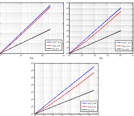
is very small compared to #(Sk,d) = d+kkfor large values of d. On Figure 1, we
provide a comparison between #(Sk,d),KL(Sk,d) and (#(Sk,d))2for various dimensions.
It is interesting to see if the estimates on the quantityK(PΛ) can be improved when using other standard probability measures over Γ. In what follows, we study this quantity when the measure
ρis the tensorized Chebyshev measure, i.e.
dρ:=⊗d j=1%(yj)dyj, with %(t) := 1 π 1 √ 1−t2. (69)
Using in this case the notationKT(Λ) =K(PΛ), we have
KT(Λ) := X ν∈Λ |Tν|2 L∞(Γ)= X ν∈Λ kTνk2L∞(Γ), (70)
whereTν(y) =Qj≥1Tνj(yj) is the tensorization of the Chebyshev polynomials (Tk)k≥0normalized
according to
Z 1
−1
|Tk(t)|2%(t)dt= 1. (71)
It is easily checked that these polynomials are related to the classical Chebyshev polynomials of the first kind byTk(cosθ) =
√
2 cos(kθ) for anyk≥1 andT0= 1. It follows that
KT(Λ) = X ν∈Λ
100 101 102 103 100 101 102 103 104 105 #Λ (#Λ)2 , d=2 K(Λ), d=2 #Λ, d=2 100 101 102 103 104 105 100 101 102 103 104 105 106 107 108 109 #Λ (#Λ)2 , d=4 K(Λ), d=4 #Λ, d=4 100 101 102 103 104 105 106 107 100 102 104 106 108 1010 1012 1014 #Λ (#Λ)2 , d=8 K(Λ), d=8 #Λ, d=8
Figure 1. Comparison between #(Λ), KL(Λ) and (#(Λ))2 in the case where
Λ =Sk,d (see (66)). Left: d= 2. Center: d= 4. Right: d= 8.
where supp(ν) := {1 ≤ j ≤d :νj 6= 0} is the support ofν ∈ F. Givenν in Λ, with Λ being a
lower set, the multi-indexµ that has the same support asν and has entries 1 satisfies µ≤ν, so that µ∈Λ andRµ⊂Λ. This implies that 2#(supp(ν))= #(Rµ)≤#(Λ). Therefore we obtain
KT(Λ)≤(#(Λ))2, (73)
which is the same bound as for the uniform measure.
Sharper bounds can be established by a finer analysis. We first prove an elementary lemma.
Proposition 1. For any real positive numbersa0≥a1≥...≥ak and any α≥ln 3ln 2, one has
aα0+ 2(aα1+. . .+aαk)≤(a0+. . .+ak)α. (74) Proof: We use induction on k. For k= 0, equality holds in (74). For k= 1, since the function
x7→(x+a1)α−xα is increasing in [a1,+∞[ then its value ata0 is greater than its value ata1, that is
2aα1 ≤(2α−1)aα1 ≤(a0+a1)α−aα0 (75)
where we have used 2α>3. Now letk≥1 anda
0≥a1≥...≥ak+1 be real positive numbers. By the induction hypothesis at steps 1 andk, we infer
(a0+...+ak+1)α = (a0+...+ak) +ak+1 α ≥(a0+...+ak)α+ 2aαk+1 ≥aα 0+ 2(aα1...+aαk) + 2aαk+1 =aα0+ 2(aα1...+aαk+1). (76)
The proof is then complete.
Lemma 2. For any lower set Λ⊂ F, the quantity KT(Λ)satisfies KT(Λ)≤(#(Λ))β, with β=
ln 3
ln 2. (77)
Proof: We use induction on nΛ := #(Λ). WhennΛ = 1, then Λ ={0F} and an equality holds.
Letn≥1 and Λ denote a lower set with nΛ=n+ 1. Without loss of generality, we suppose that
ν16= 0 for someν ∈Λ. DefiningJ ≥0 and the sets Λk as in the proof of Lemma 1 and using the
induction hypothesis with these sets, we obtain
KT(Λ) = J X k=0 γ(k)KT(Λk)≤ J X k=0 γ(k)(#(Λk)) ln 3 ln 2, (78)
whereγ is defined byγ(0) = 1 andγ(k) = 2 fork≥1. Using (74), we infer
KT(Λ)≤(#(Λ0)) ln 3 ln 2+ 2 J X k=1 (#(Λk)) ln 3 ln 2 ≤ #(Λ0) + #(Λ1) +· · ·+ #(ΛJ) ln 3ln 2 = (#(Λ))ln 3ln 2. (79)
The proof is then complete.
The bound (77) is sharp for certain type of lower sets. For instance ifν is the multi-index such that ν1=· · ·=νJ = 1 andνj = 0 forj > J, then
KT(Rν) = X µ≤ν 2#(supp(µ))=X µ≤ν 2µ1+···+µJ = J Y j=1 (1 + 2) = 3J= (2J)β = (#(Rν))β. (80)
In the case of finite dimensiond <+∞, the following bound can be easily obtained from the result of Lemma 2: KT(Λ)≤min n (#(Λ))ln 3ln 2,2d#(Λ) o .
Let us mention that similar algebraic bounds can also be obtained when the measureρis of the more general type
dρ:=⊗d j=1%(yj)dyj, %(t) = (1−t)α1(1 +t)α2 R1 −1(1−t) α1(1 +t)α2dt , α1, α2>−1, (81)
that is, the tensorization of theβ(α1, α2) measure. In this case, the relevant quantity,
KJ(Λ) = X ν∈Λ |Jα1,α2 ν | 2 L∞(Γ), (82) where Jα1,α2
ν are the tensorized Jacobi polynomials. For this quantity, the following has been
proven in [19], in the case where α1, α2 are natural exponents.
Lemma 3. For any lower set Λ ⊂ F, the quantity KJ(Λ) with Jacobi polynomials (Jαν1,α2)ν∈Λ
andα1, α2∈N0 satisfies
Note that this result includes the estimateKL(Λ)≤(#(Λ))2as the particular caseα1=α2= 0. Combining the estimates onKT(Λ) andKJ(Λ), with the results stated in the previous section, we
arrive at our main theorem for multivariate polynomial least-squares.
Theorem 3. For any r > 0, given a finite lower set Λ, if the measure ρ is the tensorized
beta(α1, α2)withα1, α2∈N0 and
n
lnn ≥
1 +r
ζ (#(Λ))
2 max{α1,α2}+2 (84)
or, if the measureρis the tensorized Chebyshev measure and
n lnn ≥ 1 +r ζ (#(Λ)) ln 3 ln 2, (85)
then the following holds true:
(i) The deviation between GandIsatisfies
Pr |||G−I|||> 1 2 ≤2n−r. (86)
(ii) Under the deterministic noise model, if usatisfies a uniform boundboverΓ, then one has
the estimate in expectation
E(ku−w˜k2)≤(1 + 2(n))em(u)2+ (8 + 2(n))kηk2+ 8b2n−r, (87)
where the factor 2in front of (n)can be removed whenη= 0.
(iii) Under the same deterministic noise model, one also has the estimate in probability Prku−wk ≥(1 +√2)em(u)∞+ 2
√
3kηkL∞
≤2n−r. (88)
4.
Discrete least-squares approximation of Hilbert space-valued
functions
In sections 2 and 3, the functions that we propose to approximate using the least-squares method are real valued. Motivated by the application to parametric PDEs, we investigate the applicability of the least-squares method in the approximation ofX-valued functions, withX being any Hilbert space. Similar to§2, we work in the abstract setting of a probability space (Γ,Σ, ρ). We study the least-squares approximation of functionsubelonging to the Bochner space
L2(Γ, X, ρ) := u: Γ→X,kuk:= Z Γ ku(y)k2Xdρ(y)<+∞ . (89)
ThereforeL2(Γ, X, ρ) =X⊗L2(Γ, ρ) and we are interested in the least-squares approximation in spaces of typeX⊗Vm whereVmis anm-dimensional subspace ofL2(Γ, ρ). Givenu∈L2(Γ, X, ρ)
an unknown function and (zi)
i=1,···,nnoiseless or noisy observations ofuat the points (yi)i=1,···,n
where the yi are i. i. d. random variables distributed according to ρ, we consider the discrete
least-squares approximation w:= argmin v∈X⊗Vm n X i=1 kzi−v(yi)k2 X. (90)
The purpose of this section is to briefly discuss the extension of the results from §2 to this frame-work.
LetBL be an orthonormal basis of the spaceVmwith respect to the measureρand consider the
matricesGandJand the familyBπ⊆Vmobtained from the basis BL and the points (yi)i=1,...,n
as in§2. When the matrixGis not singular, we claim that the solution to (90) has the same form
n X k=1
zkπk, (91)
withzk∈X for allk= 1, . . . , n, as in the real-valued case. Indeed, for anyg∈X, the real-valued
functionwg :=Pnk=1hzk, giπk ∈Vm is the solution to the least-squares problem
wg= argmin h∈Vm n X i=1 |hzi, gi −h(yi)|2, (92)
which implies the orthogonality relations
n X i=1 h n X k=1 zkπk(yi), gLj(yi)i= n X i=1 hzi, gLj(yi)i, g∈X, j∈ {1,· · ·, m}, (93)
showing thatPnk=1zkπk is the solution to (90). When the matrixGis singular, the solution (90)
is non-unique and we set by conventionw:= 0.
The explicit formula of the least-squares approximation (90) being established, we are interested in the stability and accuracy of the approximation. Similarly to the analysis in§2, we investigate the comparability over X⊗Vmof the normk · kand its empirical counterpartk · kn defined by
kvkn= 1 n n X j=1 kv(yj)k2 X 12 , v∈L2(Γ, X, ρ). (94)
It is easily checked that givenv:=
m X j=1 vjLj ∈X⊗Vm, one has kvk2 n− kvk2= m X i=1 m X j=1 (G−I)ijhvi, vjiX=hv,(G−I)viXm, (95)
wherev:= (v1,· · ·, vm)t∈Xmand the matrix-vector product is defined as in the real case. Here
the inner product h·,·iXm is the standard inner product over Xm constructed fromh·,·iX. Note
that we havekvk=kvkXm. We next observe that ifM is an m×m real symmetric matrix, one
has
sup
kvkXm=1
|hv,MviXm|=|||M|||, (96)
where |||M||| is the spectral norm of M (this is immediately checked by diagonalizing M in an orthonormal basis). Therefore it holds that
kvk2
n− kvk
and, similarly to the results discussed in §2, we find that under condition (33) the norm k · kand its counterpartk · kn are equivalent overX⊗Vm with probability greater than 1−2n−r, with
kvk 2 n− kvk 2 ≤ 1 2kvk 2. (98)
Similar to real valued functions, we want to compare the accuracy of the least-squares approxima-tion (90) with the error of best approximaapproxima-tion inL2(Γ, X, ρ)
em(u) := inf v∈X⊗Vm
ku−vk=ku−Pmuk, (99)
wherePmis the orthogonal projector ontoX⊗Vm.
We again use the notationPn
mufor the least-squares solution in the noiseless case. Ifusatisfies
a unifom bound ku(y)kX ≤ b over Γ where b is known, we define the truncated least-squares
approximation
˜
w=Tb(w), (100)
also denoted by ˜Pn
mu in the noiseless case, where Tb is the trunction operator, now defined as
follows Tb(v) = v if kvk ≤b, v kvkb ifkvk> b. (101)
Note that Tb is the projection map onto the closed disc {kvk ≤ b} and is therefore Lipschitz
continuous with constant equal to 1.
With such definitions, the result of Theorem 1 remains valid for Hilbert space valued functions with the exact same proof as for real valued functions. Likewise, with
em(u)∞= inf
v∈X⊗Vm
ku−vkL∞(Γ,X)
Theorem 2 remains valid for Hilbert space valued functions with the exact same proof as for real valued functions. In turn, the approximation results listed in (i) and (ii) of Theorem 3 are also valid for multivariate polynomial least-squares applied to Hilbert space valued functions.
As a general example of application, consider the model stochastic elliptic boundary value problem (9) with a diffusion coefficient given by (10) and satisfying (11). As recalled in the introduction, if (kψjkL∞(D))j≥1 ∈ `p(N) for some p < 1, then there exists a nested sequence of
lower sets
Λ1⊂Λ2⊂ · · · ⊂ F, #(Λm) =m, (102)
such that withX :=H1
0(D) andVm:=PΛm one has
em(u)≤Cm−s, s:=
1
p−
1
2 >0. (103)
Since the solution satisfies the uniform boundku(y)kX≤b:= kfkV
∗
r , we can compute its trunctated
least-squares approximation ˜Pmnubased onn observationsui=u(yi) where the yi are i.i.d. with respect to the uniform measure over Γ := [−1,1]N. Combining Theorem 1 for the noiseless model and (58), it follows that
E(ku−P˜mnuk
provided that lnnn ≥ m2
κ withκ:=
1−ln 2
2+2r. In particular, takingr=s, we obtain the estimate
E(ku−P˜mnuk
2)<
∼m−2s. (105)
Taking the minimal amount of samplensuch that lnnn ≥ m2
κ , this gives the convergence estimate
E(ku−P˜mnuk 2)< ∼ n lnn −s . (106)
Remark 1. The error in the evalution of u(yi) due to space discretization can be taken into
account in several ways. In the case where the space discretization is independent of the parameter
y, for example if one uses the same finite element space Xh independently of y, we may view
the polynomial least squares approximation as the noiseless approximation P˜n
muh of the discrete
solution map y7→uh(y)∈Xh. This allows to decompose the total error into
ku−P˜mnuhk ≤ kuh−P˜mnuhk+εdisc, (107)
where the second termεdisc is a uniform bound on the space discretization error, and where similar
convergence bounds to (106) can be obtained for the first term. An analogous approach was used
in [5] for the analysis of polynomial approximation obtained by truncated Taylor series. However,
in the more general case where the space discretization varies for different values ofy, one cannot
apply this strategy and a better adapted approach is to view the space discretization error as an additive deterministic noise in the observation model. Using Theorem 1 we then obtain the same
estimate as(106)for the errorku−w˜k, wherew˜ is the truncated polynomial least squares estimate
based on the discretized solution intances, up to the addition of the uniform bound εdisc on the
space discretization error. Both approaches therefore lead to the same type of estimate, but the second one applies to more general settings.
Remark 2. An analysis of the Chebyshev coefficients of u reveals that the same approximation
rate as (103) holds for theL2 norm with respect to the tensorized Chebyshev measure. However,
in view of (77), the condition betweenm andnis now lnnn ≥ mβ
κ withβ:=
ln 3
ln 2. It follows that the
rate in (106)can be improved into
E(ku−P˜mnuk 2)< ∼ n lnn −2 ln 3ln 2s , (108)
if we use samples yi that are i.i.d. with respect to the tensorized Chebyshev measure and if we
use theL2 error with respect to this measure. However, since theL2-norm with Chebyshev weight
controls the L2-norm with the uniform weight, i.e. kukL2
unif ≤
p
π/2kukL2
Cheb, estimate (108)
holds also withL2 norm with uniform weight.
5.
Application to elliptic PDEs with random inclusions
In this section, we focus on the subclass of stochastic PDEs (9)–(10) characterized by functions
ψj having nonoverlapping support. This situation allows to model, for instance, the diffusion
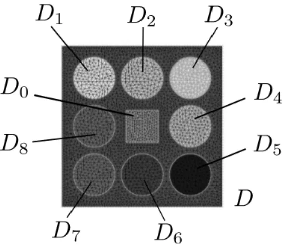
process in a medium with nonoverlapping inclusions of random conductivity (seee.g. Fig. 2). We show in what follows that exponential bounds for the discrete least-squares approximation error
in expectation can be obtained, in this case, however under a slightly more demanding condition
n ∼ m2+1/d than what shown in the previous section for algebraic convergence rates. It has
been shown in [4] that the solution map u = u(y) admits a holomorphic complex continuation
u∗:Cd→H1
0(Ω) in a polyellipse Ed ⊂Cd, whereEd =Ed(g1, . . . , gd) := Qd
n=1En,gn and En,gn :=
{z ∈ C, Re(z) = cosh(2gn) cos(θ), Im = sinh(2gn) sin(θ), θ ∈ [0,2π)} and such that Bu :=
supz∈E
dku
∗(z)k
H1
0(Ω) ≤ +∞. In this case, a priori estimates on the Legendre coefficients have
been obtainede.g. in [4] and have been shown numerically to be quite sharp. They read:
kuνkX≤C d Y j=1 exp{−νjgj}, ∀ν= (ν1, . . . , νd)∈Nd0, with X = H1
0(D), where C depends on d, (g1, . . . , gd) and Bu. Explicit expressions for the
constant Ccan be found in [4, Corollary 9 (with = 1/2)]. In practice, the coefficients (gj)1≤j≤d
can be estimated through ana posteriori procedure, that requires to solve only “one-dimensional” problems, i.e. analyzing the convergence when considering one random variable at a time and freezing all other variables to their expected value. As a consequence, quasi-optimal index sets associated with the problems in the aforementioned class are of the form
Λw=nν∈Nd0 : d X j=1 gjνj ≤w o , w = 0,1, . . . (109)
and correspond to anisotropic total degree spaces,i.e. the anisotropic variants of (66). Analogous estimates, showing the optimality of the total degree space, have been presented in [5].
In the remaining discussion, we consider the simple isotropic case where gj = g for all j =
1, . . . , d. Observe that this analysis can also be taken as a (crude) upper bound for the anisotropic case by taking g= minjgj. For convenience we introduce the following quantity:
φ:= C 2 (1−e−g)d exp ( 2e g d(1−e−1) 5 ) . (110)
Then, from the results in [4] the following estimate of the exactL2 projection error holds.
Lemma 4. In the isotropic case, i.e. gj =g for all j= 1, . . . , d, the following estimate holds for
the error of theL2 projectionPmon the quasi-optimal lower sets (109) with#(Λ) =m:
ku−Pmuk2≤φexp n
−g d e−1m1/do (111)
for any m >(2e/5)d.
Proof. The following estimate has been obtained in [4, Theorem 22]:
ku−Pmuk2≤ C2 (1−e−g)d exp n −g d e−1ln(1−ξ(m))−1m1/do, (112) with ξ(m) := (1−e−1) 1− 2e 5m1/d . (113)
Observe that we have omitted the factorCopt appearing in the mentioned theorem, as we look at the L2 projection error and not at the Galerkin error. If (2e/5)d < mthen (1−ξ(m))<1, and
the exponential term on the right-hand side in (112) can be bounded as
(1−ξ(m))gde −1m1/2 = e−1+2e(1−e −1) 5m1/d gde−1m1/d = exp{−g d e−1m1/d} 1 +2e 2(1−e−1) 5m1/d gde−1m1/d <exp 2e(1−e−1) 5 g d exp{−g d e−1m1/d}, (114)
and using the definition of φwe finally obtain the thesis.
Using the previous result and (87), we can now analyze the convergence in expectation of the discrete least-squares approximation based onnnoiseless observationsui=u(yi) where (yi)1≥i≥n
are i.i.d. with respect to the uniform measure over Γ := [−1,1]d. In particular, the parameter r
appearing in (87) has to be properly chosen as a function of nto balance the two error terms in (87). This leads to a conditionn∼m2+1/d.
Theorem 4. In the aforementioned PDE model class, when the number of points n distributed
according to the uniform measure is related to the cardinality m of the polynomial space by the
relation n≥ 2g d e ζ m 2+1 d, with ζ=1−ln 2 2 , (115)
then the convergence rate of the discrete least-squares approximation with an optimal choice of the polynomial space satisfies
E ku−P˜mnuk2≤(1 +(n)) ˜φ+ 8b2exp ( − (g d e−1)2dζ n 2 2d1+1) , (116)
with φ˜:=φexp{gde−1}.
Proof. We start from (87) in the noiseless case η = 0, and recall that, in the case of uniform
measure and polynomial spaces with downward closed index sets Λ, the cardinality of the set
m= #Λ should satisfy (84) (for α1=α2= 0). For a givennwe now take
m= $ ζ 2r n lnn 12% (117)
which satisfies (84) for any r ≥ 1. To achieve the fastest convergence, the value of r can be optimally selected as a function of the remaining parametersn,ζ,gandd. Replacing (117) in the
right-hand side of (111), we obtain for the bestL2 approximation error and anyr≥1 ku−Pmuk2≤φexp −gd e $ ζn 2rlnn 12% 1 d ≤φexp −gd e ζn 2rlnn 12 −1 !1d ≤φ˜exp ( −gd e ζn 2rlnn 21d) . (118)
Since we have embedded the stability condition (84) as a constraint, we can apply (87) in the noiseless caseη= 0 and use (118) to bound the best approximation error. Hence we obtain
E ku−P˜mnuk2≤(1 +(n)) ˜φexp ( −gd e ζn 2rlnn 21d) + 8b2 exp{−rlnn}. (119)
Now we can chooseras a function ofnanddsuch that the exponents of the two exponential terms in (119) are equal,i.e.
r= 1 lnn (g d e−1)2dζ n 2 2d1+1 . (120)
Finally, substituting this expression ofrinto (119) gives (116), which holds under condition (115) that is obtained after replacing (120) into (117).
In (116) we observe that the error converges to zero sub-exponentially as exp{−αn2d1+1} with
α:= (dg/e)2d2+1d (ζ/2) 1
2d+1. The dimensiondappears both in the factorα, favoring the convergence,
and in the exponent of n2d1+1, slowing down the convergence. A comparison with the convergence
rate of the best m-term exact L2 projection reveals that, to achieve the optimal exponential convergence rateO(exp{−gde−1m1/d}) in terms of the dimension of the polynomial space, one has to use a number of observations that scales asn∼m2+1/d.
6.
Numerical experiments
In this section we present some numerical examples that confirm the theoretical findings presented in Sections 2–5. In particular, we check that the convergence rate (116) is sharp when the number of sampling pointsnis chosen as in (115).
We consider the elliptic model (9) on the bounded domain D ⊂R2 with the random diffusion coefficienta defined in (121) by means of the geometry displayed in Fig. 2. The eight inclusions
D1, . . . , D8are circles with radius equal to 0.13, and are centered in the pointsx= (0.5,0.5±0.3),
x= (0.5±0.3,0.5) andx= (0.5±0.3,0.5±0.3). The 0.2-by-0.2 inner squareD0lies in the center ofD. The forcing termf is equal to 100 inD0and zero inD\D0. The random diffusion coefficient depends on ad-dimensional uniform random variableY ∼ U([−1,1]d), and is defined as
a(x, y) = ( 0.395 (yi+ 1) + 0.01, x∈Di, i= 1, . . . ,8, ∀y∈Γ, 1, x∈D\ ∪8 i=1Di, ∀y∈Γ, (121)
such that each component of the random variable is associated with an inclusion. The range of variation of the coefficient in each inclusion is therefore [0.01,0.8], of course satisfying the uniform
ellipticity assumption 11. All inclusions have therefore a similar influence on the solution (isotropic setting). This test case has been used in [3], and allows a direct comparison of our results with those obtained when employing the classical stochastic Galerkin method. The univariate convergence rate g= 1.9 of this example has been estimated in [4, Fig.7-left].
We consider the following quantity of interest related to the solution of the elliptic model (9),
Q(u(Y)) = 1
|D|
Z
D
u(x, y)dx,
and present the results obtained when approximating this function on polynomial spaces of fixed total degree. Similar results hold also with other quantities of interest, see [21]. We consider three cases withd= 2,d= 4,d= 8 independent random variables. In the cased= 2, the first random variable describes the diffusion coefficient in the four inclusions at the top, bottom, left, right of the center squareD0. The second random variable describes the diffusion coefficient in the other four inclusions. In the case d= 4, each one of the four random variables is associated with two opposite inclusions with respect to the center of the domain. Whend= 8 each one of the random variables is associated with a different inclusion.
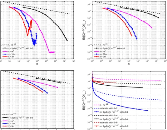
Fig. 3 shows the convergence plots obtained by the discrete least-squares approximation using a number of samples as in (115). The theoretical bound (116) is also shown as well as the reference slopen−1/2 of a standard Monte Carlo method. In the same figures we also show the convergence plots obtained when using a simple linear proportionalityn= 3morn= 10m.
Figure 2. Mesh discretization and geometries of the inclusions. The domainD is the unitary square. The inner square is namedD0, the eight circular inclusions areD1, . . . , D8.
We investigate the behaviour of the L∞ approximation error of the discrete least-squares pro-jection, approximated as E kQ(u)−P˜mnQ(u)k∞ ≈E kQ(u)−P˜mnQ(u)kcv ,
employing the cross-validation procedure described in [20, Section 4]: the expectation in the pre-vious formula is estimated by a sample average of the discrete least-squares approximation error
100 101 102 103 104 105 106 107 108 10−16 10−14 10−12 10−10 10−8 10−6 10−4 10−2 100 n E(||Q−P m nQ|| cv ) n ∼ m−1/2 n = 2gd(eζ)−1 m2+d−1 with d=2 n = m2 n = 10m n = 3m 100 101 102 103 104 105 106 107 108 10−16 10−14 10−12 10−10 10−8 10−6 10−4 10−2 100 n E(||Q−P m nQ|| cv ) n ∼ m−1/2 n = 2gd(eζ)−1 m2+d−1 with d=4 n = m2 n = 10m n = 3m 100 101 102 103 104 105 106 107 108 10−16 10−14 10−12 10−10 10−8 10−6 10−4 10−2 100 n E(||Q−P m nQ|| cv ) n ∼ m−1/2 n = 2gd(eζ)−1 m2+d−1 with d=8 n = m2 n = 10m n = 3m 0.5 1 1.5 2 2.5 x 10⁷ 10−16 10−14 10−12 10−10 10−8 10−6 10−4 10−2 100 n E(||Q−P m nQ|| cv ) n∼ m−1/2 estimate with d=2 n= 2gd(eζ)−1m2+d −1 with d=2 estimate with d=4 n= 2gd(eζ)−1m2+d −1 with d=4 estimate with d=8 n= 2gd(eζ)−1m2+d−1 with d=8
Figure 3. ErrorE(kQ−P˜mnQkcv), testing different relations between the number
of samples n and the dimension of the polynomial space m. Top-left: d = 2. Top-right: d = 4. Bottom-left: d = 8. Bottom-right: comparison between the numerical results and the theoretical bound (116), withd= 2,d= 4 and d= 8.
using 5 independent random samples of sizen. The cross-validation error is calculated as
kQ(u)−P˜mnQ(u)kcv := max i=1,...,1000 Q(u(˜yi))− ˜ PmnQ(u(˜yi)) ,
where (˜yi)1≤i≤1000 is the set of i.i.d. cross-validation points, which is kept fixed among the 5 replicas.
The results presented in Fig. 3 show that the theoretical bound (116) predicts quite sharply the error E(ku−P˜mnuk2), when the number of sampling pointsn is chosen according to (115). The
bound accurately describes the effect of the dimension d as well, in the case of moderately high dimensions.
On the other hand, a faster convergence of the errorE(ku−P˜n
muk2) with respect tonis observed,
with the linear proportionality n∼m that yields a lower number of sampling points than (115), for a given set Λ. The efficiency of the linear proportionality has been pointed out in [21], and its importance is motivated by the impossibility to employ the number of sampling points (115) when the dimensiondis large. Fig. 3 shows that already whend= 8, the exponential gain of the bound (116) with respect to a Monte Carlo rate becomes perceivable only with an astronomical number of samples, making the choice (115) less attractive for high-dimensional “isotropic” applications, whereas a linear proportionality, even with n= 3mleads to very good results. Observe, however,
that a linear proportionality might lead to instability of the discrete least-squares projection as clearly visible in Fig. 3 (top-left) in the cased= 2.
7.
Conclusion
In this work the approximation technique based on least squares with random evaluations has been analyzed. The condition between the number of sampling points and the dimension of the polynomial space, which is necessary to achieve stability and optimality, has been extended to any lower set of multi-indices identifying the polynomial space, in any dimension of the parameter set, and with the uniform and Chebyshev densities. When the measure is uniform, this condition requires the number of sampling points to scale as the square of the dimension of the polynomial space up to logarithmic factors, to achieve optimal convergence rate in expectation or in probability. As an application of this technique, we have considered a class elliptic PDE models with of “inclusion-type” stochastic coefficients. In this case, exponential convergence rates in expectation can be derived, which require, however, a slightly more demanding relation between the number of sampling points and the dimension of the polynomial space. This estimate clarifies the dependence of the convergence rate on the number of sampling points and on the dimension of the parameter set, and should be compared with the convergence rate of the best m-term exactL2 projection.
The numerical tests presented show that the proposed estimate is sharp, when the number of sampling points is chosen according to the condition that ensures stability and optimality. In addition, these results show that, in the aforementioned model class, a linear proportionality of the number of sampling points with respect to the dimension seems to be sufficient in high dimension to ensure the stability of the discrete projection, thus leading to faster convergence rates, although we have no rigourous explaination of this fact.
References
[1] I. Babuˇska, F. Nobile and R. Tempone,A stochastic collocation method for elliptic partial differential equations with random input data, SIAM J. Num. Anal. 45:1005–1034, 2007.
[2] I. Babuˇska, R. Tempone and G. E. Zouraris,Galerkin finite element approximations of stochastic elliptic partial differential equations, SIAM J. Numer. Anal. 42:800–825, 2004.
[3] J. B¨ack, F. Nobile, L. Tamellini and R. Tempone,On the optimal polynomial approximation of stochastic PDEs by Galerkin and Collocation methods, Math. Mod. Methods Appl. Sci. 22(9):1250023 (33 pages), 2012. [4] J. Beck, F. Nobile, L. Tamellini, R. Tempone,Convergence of quasi-optimal Stochastic Galerkin Methods for
a class of PDES with random coefficients, Comput. Math. Appl., 67(4):732–751, 2014.
[5] A. Chkifa, A. Cohen, R. DeVore and Ch. Schwab,Sparse adaptive Taylor approximation algorithms for para-metric and stochastic elliptic PDEs, Math. Model. Numer. Anal., 47:253–280, 2013.
[6] A. Chkifa, A. Cohen and Ch. Schwab,High-dimensional adaptive sparse polynomial interpolation and applica-tions to parametric PDEs, Found. Comp. Math., 14:601–633, 2014.
[7] A. Chkifa, A. Cohen and C. Schwab,Breaking the curse of dimensionality in sparse polynomial approximation of parametric PDEs, to appear in J. Math. Pures Appl.
[8] A. Cohen , M A. Davenport, D. Leviatan,On the stability and accuracy of least squares approximations, Found. Comput. Math., 13:819–834, 2013.
[9] A. Cohen, R. DeVore and C. Schwab,Convergence rates of bestN-term Galerkin approximations for a class of elliptic sPDEs, Found. Comp. Math. 10(6):615–646, 2010.
[10] A. Cohen, R. DeVore and C. Schwab, Analytic regularity and polynomial approximation of parametric and stochastic PDE’s, Analysis and Applications (Singapore) 9:1–37, 2011.
[11] D. Coppersmith and T.J. Rivlin,The growth of polynomials bounded at equally spaced points, SIAM J. Math. Anal, 23(4):970–983, 1992.
[13] C. de Boor and A. Ron,Computational aspects of polynomial interpolation in several variables, Mathematics of Computation 58:705–727, 1992.
[14] C.J. Gittelson,An adaptive stochastic Galerkin method, to appear in Math. Comp. 2012.
[15] M. Kleiber and T. D. Hien,The stochastic finite element methods, John Wiley & Sons, Chichester, 1992. [16] J. Kuntzman,M´ethodes num´eriques - Interpolation, d´eriv´ees, Dunod, Paris, 1959.
[17] G. Lorentz and R. Lorentz,Solvability problems of bivariate interpolation I, Constructive Approximation 2:153– 169, 1986.
[18] G.Migliorati, Polynomial approximation by means of the random discrete L2 projection and application to
inverse problems for PDEs with stochastic data, Ph.D. thesis, Dipartimento di Matematica “Francesco Brioschi” Politecnico di Milano, Milano, Italy, and Centre de Math´ematiques Appliqu´ees, ´Ecole Polytechnique, Palaiseau, France, 2013.
[19] G.Migliorati,Multivariate Markov-type and Nikolskii-type inequalities for polynomials associated with down-ward closed multi-index sets, J. Approx. Theory, 189:137–159, 2015.
[20] G. Migliorati, F. Nobile, E. von Schwerin, R. Tempone,Analysis of discreteL2projection on polynomial spaces
with random evaluations, Found. Comp. Math., 14:419–456, 2014.
[21] G. Migliorati, F. Nobile, E. von Schwerin, R. Tempone,Approximation of Quantities of Interest in stochastic PDEs by the random discreteL2projection on polynomial spaces, SIAM J. Sci. Comput., 35(3):A1440–A1460,
2013.
[22] V. Nistor and Ch. Schwab, High order Galerkin approximations for parametric, second order elliptic partial differential equations, Report 2012-22, Seminar for Applied Mathematics, ETH Z¨urich, Math. Models Methods Appl. Sci., 23, 2013.
[23] F. Nobile, R. Tempone and C.G. Webster, A sparse grid stochastic collocation method for elliptic partial differential equations with random input data, SIAM J. Num. Anal. 46:2309–2345, 2008.
[24] F. Nobile, R. Tempone and C.G. Webster,An anisotropic sparse grid stochastic collocation method for elliptic partial differential equations with random input data, SIAM J. Num. Anal. 46:2411–2442, 2008.