Facade Reconstruction Using Multiview Spaceborne
TomoSAR Point Clouds
Xiao Xiang Zhu,
Member, IEEE
, and Muhammad Shahzad,
Student Member, IEEE
Abstract—Recent advances in very high resolution tomographic synthetic aperture radar inversion (TomoSAR) using multiple data stacks from different viewing angles enables us to gener-ate 4-D (space-time) point clouds of the illumingener-ated area from space with a point density comparable to LiDAR. They can be potentially used for facade reconstruction and deformation mon-itoring in urban environment. In this paper, we present the first attempt to reconstruct facades from this class of data: First, the facade region is extracted using the density estimates of the points projected to the ground plane, the extracted facade points are then clustered into individual facades by means of orientation analysis, surface (flat or curved) model parameters of the seg-mented building facades are further estimated, and the geometric primitives such as intersection points of the adjacent facades are determined to complete the reconstruction process. The proposed approach is illustrated and validated by examples using TomoSAR point clouds generated from stacks of TerraSAR-X high-resolution spotlight images from two viewing angles, i.e., both ascending and descending orbits. The performance of the proposed approach is systematically analyzed. To explore the possible applications, we refine the elevation estimate of each raw TomoSAR point by using its more accurate azimuth and range coordinates and the corresponding reconstructed building facade model. Compared to the raw TomoSAR point clouds, significantly improved elevation positioning accuracy is achieved. Finally, a first example of the reconstructed 4-D city model is presented.
Index Terms—Facade reconstruction, point cloud, TerraSAR-X, tomographic synthetic aperture radar (SAR) inversion (To-moSAR), 4-D city model.
I. INTRODUCTION
T
HE automatic detection and reconstruction of buildings and other man-made structures from space is becoming increasingly important with the growing number of population in urban areas. Reconstructed models can serve as a major component in the realization and generation of 4-D (space-time) or even higher dimensional dynamic city models. Urban planning and management [1], tourism [2], architecture [3], damage assessment [4], and disaster management [5] are few among their various potential application areas.Manuscript received December 7, 2012; revised May 4, 2013; accepted June 19, 2013. Date of publication August 1, 2013; date of current version March 3, 2014. This work is part of the project “6.08 4D City” funded by the International Graduate School of Science and Engineering, Tech-nische Universität München, and the German Research Foundation (DFG, Förderkennzeichen BA2033/3-1).
X. Zhu is with the Remote Sensing Technology Institute (IMF), German Aerospace Center (DLR), 82234 Oberpfaffenhofen, Germany, and also with the Chair of Remote Sensing Technology, Technische Universität München, 80333 Munich, Germany (e-mail: [email protected]).
M. Shahzad is with the Chair of Remote Sensing Technology, Technische Universität München, 80333 Munich, Germany.
Color versions of one or more of the figures in this paper are available online at http://ieeexplore.ieee.org.
Digital Object Identifier 10.1109/TGRS.2013.2273619
Recent advances in very high resolution synthetic aperture radar (SAR) imagery and its key attributes—self-illumination and all-weather capability—have attracted the attention of many remote sensing analysts in the characterization of urban environments. Various techniques have been developed that make use of SAR imagery for building detection and recon-struction. Complex building shapes surrounded by roads and other structures make building detection a challenging problem. One possible solution is to discriminate buildings from other objects using the building height and width measurements extracted from SAR imagery [6]. The key issue is then the building height retrieval. For this purpose, various methods have been developed, including using sound electromagnetic models [7], layover [8] or shadow analysis [9] and simulation-based methods [10]. In [11], an approach particularly suited for the detection and extraction of large buildings based on information acquired from interferometric SAR (InSAR) data is proposed. Stochastic model-based and low level feature-based approaches for extracting and reconstructing buildings from a single SAR intensity image are presented in [12] and [13], respectively. Wanget al.[14] presented an approach for build-ing extraction from high-resolution sbuild-ingle-aspect polarimetric SAR data. Since, in urban areas, the structures are densely packed, the appearance of one particular building is dependent on the viewing angle of the sensor. Using a single-view SAR image, it is difficult to detect buildings that have no orientation component in the sensor’s azimuth direction [15]. To overcome this limit, multiview SAR acquisitions are required. In [16], an approach for estimating building dimensions using multi-view SAR images is presented. Bolter and Leberl [17] and Thieleet al.[18] proposed methods for building reconstruction based on multiview InSAR data. Building reconstruction in context to stereoscopic SAR radargrammetric and multiview polarimetric SAR acquisitions has also been used in [19] and [20], respectively.
Due to the complex urban scenes and inherent problems of SAR images such as speckle effect and layover [21], the previously presented approaches give solutions to building reconstruction but only to some extent. Spaceborne meter res-olution SAR data, together with multipass InSAR techniques, including persistent scatterer interferometry (PSI) and tomo-graphic SAR inversion (TomoSAR), allow us to reconstruct the shape and the undergoing motion of individual buildings and urban infrastructures [22]–[25]. PSI exploits bright and long-term stable objects, i.e., the persistent scatterers (PSs). However, it is restricted to single scatterers in an azimuth–range pixel. TomoSAR, on the other hand, extends the synthetic aperture principle into the elevation and temporal domain
0196-2892 © 2013 IEEE. Personal use is permitted, but republication/redistribution requires IEEE permission. See http://www.ieee.org/publications_standards/publications/rights/index.html for more information.
for 3-D and 4-D imaging [24]–[29]. It resolves the layover problem by separating multiple scatterers along the elevation direction [24]–[26], [28]. Without any preselection of pixels as PSI does, TomoSAR offers tremendous improvement in detailed reconstruction and monitoring of urban areas, par-ticularly man-made infrastructures [24]. Experiments using TerraSAR-X high-resolution spotlight data stacks show that the scatterer density obtained from TomoSAR is on the order of 600 000–1 000 000/km2 compared to a PS density on the order of40 000–100 000PS/km2[23], [24]. The rich scatterer information retrieved by TomoSAR from multiple viewing angles enables us for the first time to generate 3-D point clouds of the illuminated area with a point density comparable to LiDAR [23], [30]. These point clouds can be potentially used for building facade reconstruction in urban environment from space with the following considerations:
1) TomoSAR point clouds reconstructed from spaceborne data have a moderate 3-D positioning accuracy on the order of 1 m [31], while (airborne) LiDAR provides accu-racy typically on the order of 0.1 m [32]. Due to limited orbit spread and the small number of images, the location error of TomoSAR points is highly anisotropic with an elevation error typically one or two orders of magnitude higher than in range and azimuth. Another peculiarity of TomoSAR and PSI point clouds is that, due to multiple scattering, ghost scatterers may be generated that appear as outliers far away from a realistic 3-D position [33]. 2) Due to the coherent imaging nature and side-looking
geometry, TomoSAR point clouds emphasize different objects than LiDAR: 1) The side-looking SAR geometry enables TomoSAR point clouds to possess rich facade in-formation, and results using pixelwise TomoSAR for the high-resolution reconstruction of a building complex with very high level of detail from spaceborne SAR data are presented in [34]; 2) temporarily incoherent objects, e.g., trees, cannot be reconstructed from multipass spaceborne SAR image stacks; and 3) to obtain the full structure of individual buildings from space, facade reconstruction using TomoSAR point clouds from multiple viewing angles is required [35], [36].
3) Complementary to LiDAR and optical sensors, SAR is so far the only sensor capable of providing the fourth dimen-sion information from space, i.e., temporal deformation of the building complex [37], and microwave scattering properties of the facade reflect geometrical and material features.
However, in order to provide a high-quality spatiotemporal 4-D city model, object reconstruction from these TomoSAR point clouds is emergent. Motivated by these chances and needs, in this paper, we attempt to detect and reconstruct the building facades from TomoSAR point clouds.
Three-dimensional object reconstruction techniques from point clouds are widely employed using LiDAR data. They mostly make use of the fact that man-made structures such as buildings usually have parametric shapes. After selecting local sets of coplanar points using 3-D Hough transform or random sample consensus algorithms, 3-D objects are
recon-structed by surface fitting in the segmented building regions [38]. Numerous methods are employed for building roof seg-mentation and reconstruction such as unsupervised clustering approaches [39], region growing algorithms [40], and graph-based matching techniques [41]. These techniques, however, cannot be directly applied to TomoSAR point clouds due to different object contents captured by the side-looking SAR as mentioned earlier.
In this paper, we present an approach for the detection and reconstruction of building facades from these unstruc-tured TomoSAR point clouds. It consists of three main steps, including facade detection and extraction, segmentation, and reconstruction: First, the facade region is extracted by ana-lyzing the density of the point projected to the ground plane, the extracted facade points are then clustered into segments corresponding to individual facades by means of orientation analysis, and surface (flat or curved) model parameters of the segmented building facades are further estimated. Furthermore, we refine the elevation estimate of each raw TomoSAR point by using its more accurate azimuth and range coordinates and the corresponding reconstructed surface model of the facade. The proposed approach is illustrated and validated by examples us-ing TomoSAR point clouds generated from stacks of TerraSAR-X high-resolution spotlight images from two viewing angles, i.e., both ascending and descending orbits.
This paper is structured as follows. Section II introduces the facade surface model assumptions and describes the data set used in this paper. In Section III, the proposed approach is pre-sented, and the different processing steps are described in detail. In Section IV, the results obtained on the test buildings using TomoSAR point clouds generated from multiple viewing angles are presented, and the performance of the proposed approach is analyzed. Two application examples of the reconstructed facade models are presented in Section IV. Finally, in Section V, some conclusions are drawn, and future perspectives are outlined.
II. MODELASSUMPTION AND THEDATASET
A. Model Hypotheses/Assumptions
Many existing approaches assume polyhedral building struc-ture, i.e., roofs as planar surfaces and facades as vertical flat planes. The building model is then described by vertex points determined from intersections of ridges and boundary line segments. In most cases, the building footprint is assumed to be a rectangle polygon. As a consequence, boundary tracing algorithms usually regularize the identified boundary points to straight line segments such that the building footprints represent a polygonal shape. In our work, we assume the facades to be vertical but model their footprints by polynomial lines to allow a wider variety of architecture.
B. Data Set
The data set used in this paper is TomoSAR point clouds generated from two stacks (each comprising 25 images) of TerraSAR-X high-resolution spotlight images from ascending (36◦incidence angle) and descending (31◦incidence angle) or-bits as reported in [34]. Due to the different scattering properties
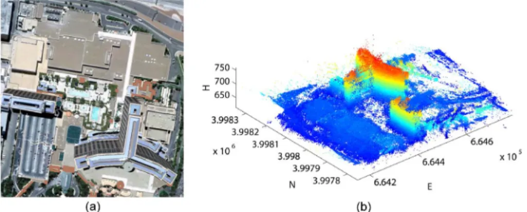
Fig. 1. Test buildings—Bellagio hotel, Las Vegas. (a) Optical image (Google). (b) Fused TomoSAR point clouds from both ascending and descending orbits in UTM coordinates.
from different geometries, there is little chance to identify a common reference point for both stacks. This problem results in a shift in the elevation directions of both point clouds recon-structed from these two stacks with different viewing angles. To obtain the full structure of individual buildings from space, the point clouds are first geodetically fused by determining this shift in elevation direction [30], [42]. The proposed facade reconstruction approach is then applied to the resulting fused point clouds. Fig. 1(a) shows the optical image of our test buildings, the Bellagio hotel complex in Las Vegas. Fig. 1(b) gives an overview of the fused input TomoSAR point cloud in universal transverse mercator (UTM) coordinates. The size of the test area is about520×570m2. The number of TomoSAR
points is approximately 0.4 million. III. METHODOLOGY
As illustrated in Fig. 2, the proposed approach consists of three main steps, including facades detection and extraction, segmentation, and reconstruction.
A. Facade Detection and Extraction
Building facade detection and extraction is generally the first and important step toward the reconstruction of 3-D building models from point clouds generated from aerial or spaceborne acquisitions. A common approach in LiDAR point cloud pro-cessing is to first compute a (or use an already existing) digital terrain model (DTM) by filtering techniques, e.g., morphologi-cal filtering [43]–[45], gradient analysis [46], or iterative densi-fication of triangular irregular network structure [47], [48], and then use the DTM to extract nonground points [49], [50] from the rasterized point cloud data. The rasterized nadir-looking LiDAR point cloud gives a digital surface model (DSM). The difference of DSM and DTM provides us a normalized DSM that gives us the height variations among nonground points. By exploiting geometrical features such as deviations from the surface model [51], local height measures [32], [45], roughness [45], and slope variations [43], [46], building points can be ex-tracted out. Some methods support the building detection prob-lem by explicitly using 2-D footprints [52], [53]. They help in reducing the building detection problem by providing the build-ing regions but can suffer from inaccurate positionbuild-ing accuracy [54] and artifacts introduced during data acquisition [38].
Fig. 2. Workflow of the proposed approach.
Our proposed approach for extracting building facades ex-ploits the idea of orthogonally projecting the points onto the 2-D ground plane as presented in [38]. However, instead of estimating local planes to refine the building outline, the 2-D scatterer (point) density (SD) in the horizontal x–y (ground) plane is used to extract facade points. The proposed method works directly on the unstructured 3-D TomoSAR points. SD is locally estimated for each grid point defined on the ground plane by first accumulating the number of points within a local window and then dividing by the window size. By exploiting the fact that, for a side-looking instrument like SAR, the point density is much higher for vertical structures (value depending on the building height), the building facades are extracted.
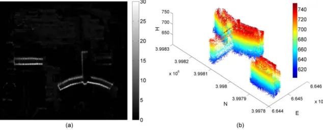
Fig. 3(a) shows the SD map of the input TomoSAR point cloud shown in Fig. 1(b). The grid spacing is set to1×1m2. The grid cells having a point density less than a specified threshold T H are removed. A mask is then generated after a morphological dilation which, in turn, is used for building
Fig. 3. Facade (detection) extraction. (a) Scatterer density map in the ground plane on a1×1m2grid. (b) Extracted building facade points. The color bar
indicates the (a) number of points/m2. (b) Sea-level height in meters of each 3-D building facade point. (facade) point extraction in each grid cell. Fig. 3(b) shows
the extracted points belonging to the facades of two different buildings. The number of buildings in the scene is found by analyzing the footprint in the generated mask (which is two in our case).
B. Segmentation
To reconstruct individual facades, the segmentation of the points belonging to the same facade is required. Most seg-mentation approaches make use of unsupervised clustering techniques. They typically search for local plane features and then perform neighborhood analysis using the detected features [38], [55]. Only considering the planar segments can be too re-strictive as in the appearance of the curved surfaces that can be better modeled using second-order or higher order polynomials. Therefore, we search for both planar and curved surfaces and further distinguish them by local footprint orientation analysis. a) Local Orientation Estimation: Given the set of pixels representing the building regions in thex–yplane, the local ori-entation angleθis estimated by weighted least squares (WLS) adjustment. The corresponding weight of the facade pixels within the estimation window is given by the corresponding estimated SD. If there is no point inside the window other than the considered point, that point is no longer considered as part of any facade footprint and hence removed. The estimated local orientation along the facade footprints for a10×10m2
window size is shown in Fig. 4. The orientation change between different facades is quite evident.
b) Feature Vector Selection: Extracted facade points from the preceding step are further clustered into segments cor-responding to individual facades. As mentioned earlier, the orientation estimates of different facade footprints are used to cluster the points. To distinguish grid pixels that are spatially far apart but having similar orientation, spatial parameters are also incorporated as features for clustering, i.e., a 3-D feature space(x, y, θ)is adopted.
c) K-Means Clustering: The well-known K-means cluster-ing algorithm is used here for segmentation with the aforemen-tioned 3-D feature vector incorporating spatial features(x, y)
and orientation angleθdepicted in Fig. 4.
Fig. 4. Orientation estimates in degrees on each grid point of Fig. 3(a). The color bar indicates the degree range[−90∼90].
A common problem related tok-means is to know the num-ber of clusters (facades)k in advance that is not pragmatic in our case. To overcome this limitation, an initial guess about the number of clusters is first computed such that it underestimates
k. The points are then clustered with the initial guess using
k-means. Points within each resulting cluster that are spatially disconnected are then further separated as smaller clusters. Based on this more detailed clustering result, the points near boundaries of adjacent facades that are normally far away from the corresponding cluster center are further finely clustered.
Initial guess about number of clusters: To determine the initial number of clusters, the within-cluster dispersion is de-termined in successive clustering runs for varying numbers of clusters.
Let us defineDras the mean deviation of points in clusterr from its respective center
Dr= nr i=1 di nr (1)
where nr is the number of points in cluster r anddi is the Euclidean distance of the ith point in r from its center. The dispersion index Ik for k clusters can then be determined as [55] Ik= k r=1 Dr k . (2)
A plot of such dispersion index against the number of clus-ters gives us an indication on how to choose an appropriate number of clusters [55]. The dispersion indexIk usually de-creases significantly with increasing number of clusters and becomes steady afterward. The location of the elbow point can be considered as a good estimate of the number of clusters [55], [56].
Separation of clusters Within clusters: With initially guessed and underestimatedk, it is common that facades hav-ing similar orientation estimates and relatively small spatial distances have been clustered into one group. It is therefore necessary to extract and treat clusters within clusters that are not spatially connected as separate clusters. For this reason, we perform a connectivity analysis to determine the number of contours and treat each contour as a separate cluster. However, if the contour is very small, i.e., the number of pixels is less thanTp, it is omitted.
Finer clustering: After separating clusters within clusters, the following procedure is adopted for refinement.
1) Appropriate polynomial models (first for flat and second for curved) are fitted to estimate the cluster footprints. Model parameters are estimated byL1 norm minimiza-tion that is robust against outliers.
2) Accept points in each corresponding cluster that are within the2σdistance from the estimated facade, where
σis the standard deviation of the residual.
3) Connectivity analysis is then carried out for the rejected points. Three possible cases can exist.
a) The point is isolated. In this case, it is removed. b) The point is connected to other discarded points. In
this case, the number of points is counted, and in case the number is less than Tp, they are removed. Otherwise, they are merged together to form a new cluster.
c) The point belongs to another cluster. In this case, the discarded point is assigned to another existing cluster. By following the aforementioned procedure, extracted facade points are clustered into segments.
C. Reconstruction
A facade is normally characterized by a flat or curved sur-face, edges (facade boundary), and the corresponding vertices. These features will be reconstructed in this section.
a) Model Identification (Flat or Curved Facade Surfaces): The facade surfaces to be modeled are first classified to flat and curved surfaces by analyzing derivatives of the local ori-entation angleθ. The curved surfaces have gradually changing orientations across their footprint compared to flat surfaces that have ideally constant orientations. We first compute the first derivativesθ of the orientation angleθ for each facade foot-print. Since the locally estimated θ is usually noisy, second-order polynomial fitting is applied for denoising. The decision on whether an individual facade footprint is flat or curved is based on the behavior ofθ. Facade footprints with too small orientation variation are considered to be flat while facade footprints with gradually changing orientation are considered to be curved.
TABLE I
PROCEDURE TOFIND THEADJACENTSEGMENTS OF APARTICULARFACADESEGMENT
b) Parameter Estimation: Finally, model parameters for each segmented facade are estimated. Each extracted point in Fig. 3(b) is assigned a weight corresponding to its SD depicted in Fig. 3(a). Two-dimensional facade footprints are then reconstructed by a WLS method. Polynomials are used to model the facade footprints in thex–yplane
fp(x, y) = p q=1
aqxiyj i+j≤q (3) where iandj are permuted accordingly,pis the order of the polynomial, and the number of terms in the above polynomial is equal to (p+ 1)(p+ 2)/2. Flat and curved surfaces are modeled using first-order (p= 1) and second-order (p= 2)
polynomial coefficients, respectively. Higher order polynomials could be used to model more complex building structures.
c) Vertex Determination: Once the facade model parameters are estimated, the final step is to describe the overall shape of the building footprint by further identifying adjacent facade pairs and determining the intersection of their facade surfaces.
The adjacency of facades is described by an adjacency matrix that is built up via connectivity analysis. Table I shows the procedure that we propose to decide the adjacency of one particular facade segment with other facade segments of the building.
Identified adjacent facade segments are then used to deter-mine the vertex points in 2-D (i.e., facade intersection lines in 3-D). They are found by computing the intersection points between any adjacent facade pair. Since polynomial models are used for facade parameter estimation, the problem of finding vertex points boils down to find the intersection point between the two polynomials corresponding to the two adjacent facades. Depending on flat or curved facades, two cases needed to be discussed.
1) Adjacent facades are flat: In this case, there is only one intersection point which is taken as the vertex point. 2) One of the two facades is curved, or both facades are
curved: There is more than one solution. In these cases, mean Euclidean distances of the possible intersection
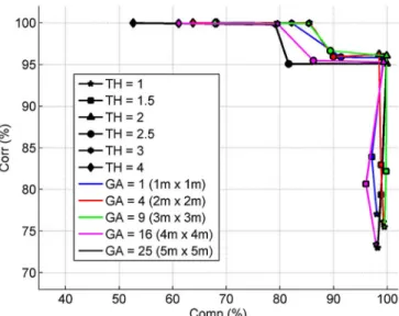
Fig. 5. Completeness versus correctness with the varying T H and GA
parameters.
points to both adjacent facades are computed. The point having the smaller mean distance to both facades is considered as the vertex point.
The computed vertex points and the estimated model param-eters are then used to finally reconstruct the 3-D model of the building facades.
IV. EXPERIMENTALRESULTS ANDVALIDATION
In this section, we discuss and assess the overall performance of the proposed method: The performance of the building facade extraction is evaluated, clustering issues are discussed, and the positioning accuracy of the facade models is further assessed.
A. Performance Assessment of Facade Extraction
To evaluate the quality of our facade extraction procedure, a pointwise comparison method is employed. Extracted facade points are compared to the reference data, and the results are analyzed for quantitative and qualitative evaluation.
Pseudoreference data: The absence of exact reference data representing the actual facade area restricts the accurate evaluation of the facade point extraction procedure, but since we are already incorporating prior knowledge (i.e., the fact that higher point density areas represent vertical structures) in estimating few facade parameters from a large number of points belonging to an individual building facade, it is highly probable that points closer to the reconstructed facade footprint are indeed points belonging to the corresponding facades. We therefore consider all points that are within 1.5σof the esti-mated facade footprints reported in Section IV-C to be true facade points and use them to assess the performance of the proposed facade extraction procedure.
Evaluation Metrics: To evaluate the performance of the proposed building facade extraction procedure, all the points in the input point cloud data are assumed to belong to one of the two categories, i.e., facade or nonfacade points. Any point detected as a facade point by the algorithm that also
TABLE II
OVERALLSUCCESS OF THEEXTRACTIONPROCEDURE INTERMS OFQUALITY FORSIXT HANDFIVEGAVALUES
corresponds to a facade in the reference data set is taken as true positive(T P). Similarly, a point labeled as a facade point but is not actually a facade point in the reference data set is treated as false positive(F P). A false negative(F N)corresponds to a point which belongs to the facade in the reference data set but is wrongly labeled as a nonfacade point by the facade extraction procedure. The performance of the (detection) extraction pro-cedure is then assessed by employing the following evaluation metrics [57], [58]: Completeness(%) : comp= 100× T P T P+F N Correctness(%) : corr= 100× T P T P+F P
Quality(%) : Q=comp+comp×corrcorr−comp×corr= T P+F PT P+F N
⎫ ⎪ ⎪ ⎬ ⎪ ⎪ ⎭ . (4) The metrics mentioned above assess the overall performance of the extraction algorithm. Completeness tells up to what percentage the algorithm has detected the facade points while correctness provides a measure of correct classification. Among them, completeness is particularly important in our application in order to preserve intact facade footprints. The quality Q
is crucial when comparing the results obtained from different algorithms [57].
Dependency on window sizeGAand thresholding param-eterT H: Two parameters that influence the number of facade points extracted by the algorithm are as follows: the threshold
T Hand window sizeGA. In order to assess the effect of these two parameters on the extraction procedure, the evaluation was carried out using the following sequence of GAs and THs, withGA={1×1,2×2,3×3,4×4,5×5}m2andT H=
{1.0,1.5,2.0,2.5,3.0,4.0}points/m2.
To characterize the performance of the extraction procedure, the dependence of completeness and correctness metrics on these two parameters is analyzed. A tradeoff between complete-ness and correctcomplete-ness can then be chosen based on the adjustable setting parameters. Fig. 5 depicts the completeness and cor-rectness achieved with differentT H andGAparameters. It is obvious that a lowerT Hvalue results in higher completeness. The higher theT Hvalue, the less the false positives observed, which results in higher correctness. This simply lies in the fact that it is more probable that the grid point with higher SD belongs to a facade. Table II gives us the overall success of the extraction procedure in terms of quality(Q)for sixT Hand five
GAvalues defined earlier. The performance of the extraction procedure is best under the following parameter settings:T H= 2points/m2andGA= 3×3m2. The overall quality of which
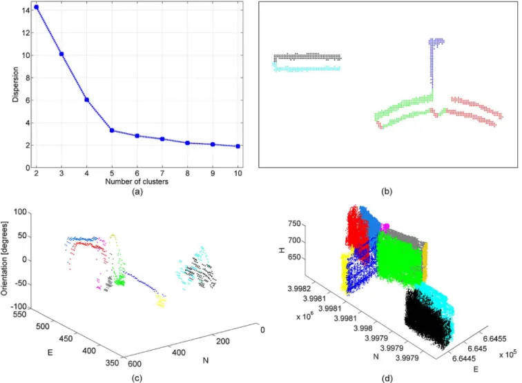
Fig. 6. Segmentation results. (a) Dispersion plot with elbow point atk= 5. (b) Corresponding clustering withk= 5. (c) Clustered grid points in feature space, i.e., orientation (in degrees) and spatial positions on the ground plane (in meters). (d) Corresponding clustered TomoSAR points.
is 95.94%. Generally better correctness and completeness can also be observed from Fig. 5 with this parameter setting, i.e., a completeness of 99.89% and a correctness of 96.04%.
Based on the aforementioned discussion, in our experiment, we estimate the SD on the ground plane with a grid distance of 1 m. The window size is set to be3×3m2. A facade mask
on the ground plane is obtained based on the resulting SD map by setting a threshold of 2 points/m2 that are finally used for facade extraction. It is worth to mention that aforementioned parameters are tuned to point clouds generated from TerraSAR-X high-resolution spotlight data, i.e., a resolution of 1.1 m× 0.6 m ×30 m, and the particular incidence angles. For other configurations, the optimal GA will be different.
B. Clustering
Extracted facade points from the previous step are further clustered into segments corresponding to individual facades. For a reasonable initial guess of the number of clusters, Fig. 6(a) shows the plot ofIk by assuming different numbers of clusters
k= 2, . . . ,10. We can observe that the dispersion index Ik decreases significantly with decreasing number of clusters with
kup to 5 and becomes steady afterward. The number of clusters at this elbow point has been chosen as the initial number
of clusters. Fig. 6(b) shows the preliminary clustering results withk= 5. It is evident that different facades having similar orientation estimates and relatively small spatial distance have been clustered in one group. Therefore, small clusters that are not spatially connected are separated. Very small contours, i.e., the number of pixels is less thanTp(Tp= 10in our case), are omitted. By following the procedure of the final fine clustering, the extracted points are clustered into ten segments. Fig. 6(c) and (d) shows the color-coded clustering of grid points in fea-ture space after refinement and their corresponding TomoSAR points in UTM coordinates, respectively.
C. Three-Dimensional Facade Reconstruction
By analyzing the orientation derivatives as described in Section III-C, the ten clustered facades in Fig. 6(d) are iden-tified as five curved and five flat facades. Each extracted facade footprint point in 2-D is assigned a weight corresponding to its SD depicted in Fig. 3(a). Two-dimensional facade footprints are then reconstructed using the WLS method.
Once the facade model parameters are estimated, the next step is to find the intersection of these facade surfaces to describe the overall shape of the building footprint. Following the procedure depicted in Table I, the corresponding adjacency
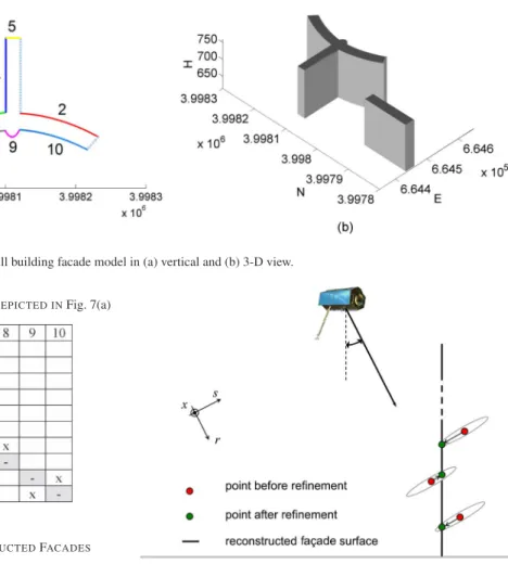
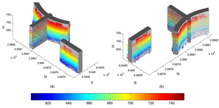
Fig. 7. Three-dimensional view of the reconstructed full building facade model in (a) vertical and (b) 3-D view. TABLE III
ADJACENCYMATRIX OF THEFACADESEGMENTSDEPICTED INFig. 7(a)
TABLE IV
STATISTICS ANDACCURACY OF THERECONSTRUCTEDFACADES
matrix for all the facade segments labeled in Fig. 7(a) is depicted in Table III. The crosses indicate the mutual adjacent facade pairs. The vertex points are found by computing the intersection points between any adjacent facade pair.
Fig. 7 shows the final reconstructed building facade mod-els using the estimated parameters and the determined vertex points. Table IV depicts the statistics of the reconstructed facades. It also assesses the accuracy of the estimated facade models by computing the root-mean-square error (RMSE) of all the points from their respective reconstructed facade. For comparison, facade parameters are also estimated by assigning
Fig. 8. Basic principle for the elevation estimate refinement of the TomoSAR points by using their more accurate azimuth and range coordinates and the reconstructed facade surfaces.
uniform weights. Compared to facade parameters estimated by assigning weights according to their SD, bigger mean RMSE is observed.
V. APPLICATIONEXAMPLES
In this section, the reconstructed model presented in Section IV is used to refine the elevation estimates of the raw TomoSAR point clouds, and an example of the reconstructed 4-D building model is presented.
A. Elevation Estimate Refinement
As briefly mentioned in Section I, due to the limited orbit spread and the small number of images, the location error of TomoSAR points is highly anisotropic with an elevation error typically one to two orders of magnitude higher than in range and azimuth. For TerraSAR-X high-resolution spotlight images with typical parameters, the theoretical relative localization precision of a PS is as follows [59]: 1.7–2.1 cm in range; 3.2–3.8 cm in azimuth, and 62–139 cm in elevation.
The elevation estimates of the TomoSAR points can be refined by using their more accurate azimuth and range coordi-nates and the identified and modeled facade surfaces as depicted in Fig. 8. This sketch illustrates the refinement principle in
Fig. 9. Elevation estimate refinement. (a) TerraSAR-X mean intensity map from ascending stacks (the red dots are the analyzed points) along with the projection geometry. Height estimates of the analyzed points (b) before and (c) after refinement.
the range–elevation plane. The red points represent the raw TomoSAR point locations at different heights along a facade. The ellipse indicates the error ellipse of the TomoSAR estimate in the range and elevation direction, i.e., much poorer accuracy in elevation compared to range. The black line indicates the reconstructed facade surface. We project the corresponding iso-azimuth-range lines of each point along elevation (directions are indicated by the arrows) to the identified and modeled facade surface that it belongs to. The final refined 3-D position is obtained by taking the elevation coordinate of the intersection point. This is an approximation of an optimal linear estimate. The green points represent the positions after elevation refine-ment. In this way, we expect to achieve much better elevation estimation accuracy that is on the order of several centimeters, although it is still slightly worse than the ones in azimuth and range due to error propagation.
To validate this improvement, we selected a row of bright points from the intensity image belonging to a facade portion of constant height as shown in Fig. 9(a). Fig. 9(b) and (c) compares the height estimates of the analyzed points before and after the refinement. It is obvious that their height estimates are improved significantly. The standard deviations before and after the refinement are 190 and 5.5 cm, respectively, an
im-provement by a factor of 35 which corresponds quite nicely to the ratio of inherent resolutions in elevation (on the order of 30–50 m) and range (1.1 m).
B. 4-D Building Model
To better monitor the detailed structures of individual build-ings, an example of the reconstructed 4-D building model is presented in Figs. 10–12. In Fig. 10, the fused point clouds with refined elevation are visualized by overplotting them onto the reconstructed facade model. The height of the points is color coded. The corresponding estimated motion parameter (in this case, the amplitude of seasonal motion caused by thermal dilation) is illustrated in Fig. 11. This information can be used for developing dynamic building models from spaceborne SAR data that can help to monitor individual buildings and even the whole city. Fig. 12 shows the reconstructed 3-D SAR image, i.e., the reflectivity map overlaid on the facade model. Such an image visualizes in detail how the Bellagio hotel would look like in X-band for our eyes, if they could sense microwaves, from the position of the SAR satellite. Such visualizations may lead to a better understanding of the nature of scattering.
Fig. 10. Point clouds with refined elevation overplotted on the reconstructed facade model. The height of the points is color coded (unit: meters).
Fig. 11. Reconstructed 4-D building facade model. The amplitude of seasonal motion is color coded (unit: millimeters).
VI. OUTLOOK ANDCONCLUSION
TomoSAR point clouds are very attractive for dynamic city model generation. As the first attempt, a facade reconstruction approach tailored to this class of data is proposed in this paper. It consists of three main steps: facade extraction, segmentation, and reconstruction. The proposed approach is illustrated by using fused TomoSAR point clouds from two stacks (ascend-ing and descend(ascend-ing) of TerraSAR-X high-resolution spotlight data. We use the reconstructed facade model to refine the
TomoSAR elevation estimates. Compared to the raw TomoSAR point clouds, significantly improved elevation positioning ac-curacy on the order of several centimeters is achieved. A first example of the reconstructed 4D building model is also presented.
There are several aspects of the proposed reconstruction procedure that can be improved in the future. Among them, the proposed approach is based on the assumption that facades are vertical and the footprint of each segment can be represented by
Fig. 12. Reconstructed 3-D SAR image overplotted on the reconstructed facade model. Note that this is not only a projection of the SAR image onto the building models. Rather, the lay-overed brightness contributions from facade and ground have been separated in the tomographic reconstruction step.
a set of polynomial coefficients. The fact that facade parameters are estimated from the segmented points makes the recon-struction performance strongly dependent on the quality of the segmentation. In our experiment, we rely on the assumption of having a high number of scatterers on the building facades and hence used the SD as the basis for various operations, including segmentation, orientation parameter estimation, and facade parameter estimation. In most cases, the assumption is valid because of the existence of strong corner reflectors, e.g., window frames, on the building facades. However, there are exceptional cases: 1) the facade structure is smooth, i.e., only very few scatterers can be detected on the facades, and 2) the building is low. In these cases, SD might not be the optimum choice. Alternatively, we can use other scatterer characteristics such as intensity and SNR for extraction and reconstruction purposes.
In the future, we will also concentrate on object-based To-moSAR point cloud fusion, building roof reconstruction, and automatic object reconstruction for large areas.
ACKNOWLEDGMENT
The authors would like to thank R. Bamler for proofreading the manuscript.
REFERENCES
[1] J. Benner, A. Geiger, and K. Leinemann, “Flexible generation of seman-tic 3D building models,” inProc. Int. ISPRS/EuroSDR/DGPF-Workshop Next Gen. 3D City Models, K. Gröger, Ed., Bonn, Germany, 2005, pp. 18– 22, EuroSDR Publication No. 49.
[2] J. Döllner, T. H. Kolbe, F. Liecke, T. Sgouros, and K. Teichmann, “The vir-tual 3D city model of Berlin—Managing, integrating, and communicating complex urban information,” inProc. 25th UDMS, Aalborg, Denmark, May 15–17, 2006, pp. 1–12.
[3] X. Yin, P. Wonka, and A. Razdan, “Generating 3D building models from architectural drawings: A survey,”IEEE Comput. Graph. Appl., vol. 29, no. 1, pp. 20–30, Jan./Feb. 2009.
[4] J. Lee and S. Zlatanova, “A 3D data model and topological analyses for emergency response in urban areas,” inGeospatial Information Technol-ogy for Emergency Response, L. Zlatanova, Ed. New York, NY, USA: Taylor & Francis, 2008.
[5] S. Kemec, S. Duzgun, S. Zlatanova, D. I. Dilmen, and A. C. Yalciner, “Se-lecting 3D urban visualization models for disaster management: Fethiye tsunami inundation case,” inProc. 3rd Int. Conf. Cartogr. GIS, Nessebar, Bulgaria, Jun. 15–20, 2010, pp. 1–9.
[6] A. Bennett and D. Blacknell, “Infrastructure analysis from high resolution SAR and InSAR imagery,” inProc. GRSS/ISPRS Joint Workshop Remote Sens. Data Fusion Over Urban Areas, 2003, pp. 230–235.
[7] R. Guida, A. Iodice, and D. Riccio, “Height retrieval of isolated buildings from single high-resolution SAR images,”IEEE Trans. Geosci. Remote Sens., vol. 48, no. 7, pp. 2967–2979, Jul. 2010.
[8] F. Tupin, “Extraction of 3D information using overlay detection on SAR images,” inProc. GRSS/ISPRS Joint Workshop Data Fusion Remote Sens. Over Urban Areas, 2003, pp. 72–76.
[9] A. J. Bennett and D. Blacknell, “The extraction of building dimensions from high resolution SAR imagery,” in Proc. Int. Radar Conf., 2003, pp. 182–187.
[10] D. Brunner, G. Lemoine, L. Bruzzone, and H. Greidanus, “Building height retrieval from VHR SAR imagery based on an iterative simulation and matching technique,”IEEE Trans. Geosci. Remote Sens., vol. 48, no. 3, pp. 1487–1504, Mar. 2010.
[11] P. Gamba, B. Houshmand, and M. Saccani, “Detection and extraction of buildings from interferometric SAR data,”IEEE Trans. Geosci. Remote Sens., vol. 38, no. 1, pp. 611–617, Jan. 2000.
[12] M. Quartulli and M. Datcu, “Stochastic geometrical modeling for built-up area understanding from a single SAR intensity image with meter resolution,”IEEE Trans. Geosci. Remote Sens., vol. 42, no. 9, pp. 1996– 2003, Sep. 2004.
[13] A. Ferro, D. Brunner, and L. Bruzzone, “An advanced technique for build-ing detection in VHR SAR images,” inProc. SPIE Conf. Image Signal Process. Remote Sens., 2009, vol. 7477, pp. 74770V-1–74770V-12. [14] Y. Wang, F. Tupin, C. Han, and J. M. Nicolas, “Building detection from
high resolution PolSAR data by combining region and edge information,” inProc. IEEE IGARSS, 2008, pp. IV-153–IV-156.
[15] J. D. Wegner, U. Soergel, and A. Thiele, “Building extraction in urban scenes from high resolution InSAR data and optical imagery,” inProc. Urban Remote Sens. Event, 2009, pp. 1–6.
[16] R. Hill, C. Moate, and D. Blacknell, “Estimating building dimensions from synthetic aperture radar image sequences,”IET Radar, Sonar Navig., vol. 2, no. 3, pp. 189–199, Jun. 2008.
[17] R. Bolter and F. Leberl, “Detection and reconstruction of human scale features from high resolution interferometric SAR data,” inProc. ICPR, 2000, pp. 291–294.
[18] A. Thiele, E. Cadario, K. Schulz, U. Thoennessen, and U. Soergel, “Build-ing recognition from multiaspect high-resolution InSAR data in urban areas,”IEEE Trans. Geosci. Remote Sens., vol. 45, no. 11, pp. 3583–3593, Nov. 2007.
[19] E. Simonetto, H. Oriot, and R. Garello, “Rectangular building extraction from stereoscopic airborne radar images,”IEEE Trans. Geosci. Remote Sens., vol. 43, no. 10, pp. 2386–2395, Oct. 2005.
[20] F. Xu and Y. Q. Jin, “Automatic reconstruction of building objects from multiaspect meter-resolution SAR images,”IEEE Trans. Geosci. Remote Sens., vol. 45, no. 7, pp. 2336–2353, Jul. 2007.
[21] U. Stilla, U. Soergel, and U. Thoennessen, “Potential and limits of InSAR data for building reconstruction in built-up areas,”ISPRS J. Photogramm. Remote Sens., vol. 58, no. 1/2, pp. 113–123, Jun. 2003.
[22] R. Bamler, M. Eineder, N. Adam, S. Gernhardt, and X. Zhu, “Interfero-metric potential of high resolution spaceborne SAR,” inProc. PGF, 2009, pp. 407–419.
[23] S. Gernhardt, N. Adam, M. Eineder, and R. Bamler, “Potential of very high resolution SAR for persistent scatterer interferometry in urban ar-eas,”Ann. GIS, vol. 16, no. 2, pp. 103–111, Jun. 2010.
[24] X. Zhu and R. Bamler, “Very high resolution spaceborne SAR tomogra-phy in urban environment,”IEEE Trans. Geosci. Remote Sens., vol. 48, no. 12, pp. 4296–4308, Dec. 2010.
[25] D. Reale, G. Fornaro, A. Pauciullo, X. Zhu, and R. Bamler, “Tomographic imaging and monitoring of buildings with very high resolution SAR data,”
IEEE Geosci. Remote Sens. Lett., vol. 8, no. 4, pp. 661–665, Jul. 2011. [26] G. Fornaro, F. Serafino, and F. Soldovieri, “Three-dimensional focusing
with multipass SAR data,”IEEE Trans. Geosci. Remote Sens., vol. 41, no. 3, pp. 507–517, Mar. 2003.
[27] F. Lombardini, “Differential tomography: A new framework for SAR interferometry,” inProc. IEEE IGARSS, Toulouse, France, 2003, pp. 1206–1208.
[28] G. Fornaro and F. Serafino, “Imaging of single and double scatterers in urban areas via SAR tomography,”IEEE Trans. Geosci. Remote Sens., vol. 44, no. 12, pp. 3497–3505, Dec. 2006.
[29] G. Fornaro, D. Reale, and F. Serafino, “Four-dimensional SAR imaging for height estimation and monitoring of single and double scatterers,”
IEEE Trans. Geosci. Remote Sens., vol. 47, no. 1, pp. 224–237, Jan. 2009. [30] S. Gernhardt, X. Cong, M. Eineder, S. Hinz, and R. Bamler, “Geometrical fusion of multitrack PS point clouds,”IEEE Geosci. Remote Sens. Lett., vol. 9, no. 1, pp. 38–42, Jan. 2012.
[31] X. Zhu and R. Bamler, “Super-resolution power and robustness of com-pressive sensing for spectral estimation with application to spaceborne tomographic SAR,”IEEE Trans. Geosci. Remote Sens., vol. 50, no. 1, pp. 247–258, Jan. 2012.
[32] F. Rottensteiner and C. Briese, “A new method for building extraction in urban areas from high resolution LIDAR data,” inProc. ISPRS Photogram. Comput. Vision, Graz, Austria, Sep. 9–13, 2002, pp. 295–301.
[33] S. Auer, S. Gernhardt, and R. Bamler, “Ghost persistent scatterers related to multiple signal reflections,”IEEE Geosci. Remote Sens. Lett., vol. 8, no. 5, pp. 919–923, Sep. 2011.
[34] X. Zhu and R. Bamler, “Demonstration of super-resolution for tomo-graphic SAR imaging in urban environment,”IEEE Trans. Geosci. Re-mote Sens., vol. 50, no. 8, pp. 3150–3157, Aug. 2012.
[35] M. Shahzad, X. Zhu, and R. Bamler, “Facade structure reconstruction us-ing spaceborne TomoSAR point clouds,” inProc. IEEE IGARSS, Munich, Germany, 2012, pp. 467–470.
[36] X. Zhu, M. Shahzad, and R. Bamler, “From TomoSAR point clouds to objects: Facade reconstruction,” inProc. TyWRRS, Naples, Italy, 2012, pp. 106–113.
[37] X. Zhu and R. Bamler, “Let’s do the time warp: Multi-component non-linear motion estimation in differential SAR tomography,”IEEE Geosci. Remote Sens. Lett., vol. 8, no. 4, pp. 735–739, Jul. 2011.
[38] P. Dorninger and N. Pfeifer, “A comprehensive automated 3D approach for building extraction, reconstruction, and regularization from airborne laser scanning point clouds,”Sensors, vol. 8, no. 11, pp. 7323–7343, Nov. 2008.
[39] S. Filin, “Surface clustering from airborne laser scanning data,”Int. Arch. Photogramm. Remote Sens. Spatial Inf. Sci., vol. 34, no. 3A, pp. 119–124, Sep. 2002.
[40] F. Ahmed and S. James, “Reconstructing 3D buildings from Lidar data,” inProc. ISPRS Commiss. III Symp., Graz, Austria, Sep. 9–13, 2002, pp. 1–6. [41] G. Forlani, C. Nardinocchi, M. Scaioni, and P. Zingaretti, “Complete classification of raw LIDAR data and 3D reconstruction of buildings,”
Pattern Anal. Appl., vol. 8, no. 4, pp. 357–374, Feb. 2006.
[42] Y. Wang, X. Zhu, Y. Shi, and R. Bamler, “Operational TomoSAR process-ing usprocess-ing multitrack TerraSAR-X high resolution spotlight data stacks,” inProc. IEEE IGARSS, Munich, Germany, 2012, pp. 7047–7050. [43] G. Sithole and G. Vosselman, “Experimental comparison of filtering
algorithms for bare-earth extraction from airborne laser scanning point clouds,”ISPRS J. Photogramm. Remote Sens., vol. 59, no. 1/2, pp. 85– 101, Aug. 2004.
[44] K. Zhang, S.-C. Cheng, D. Whitman, M.-L. Shyu, J. Yan, and C. Zhang, “A progressive morphological filter for removing non-ground measure-ments from airborne LIDAR data,”IEEE Trans. Geosci. Remote Sens., vol. 41, no. 4, pp. 872–882, Apr. 2002.
[45] F. Rottensteiner, J. Trinder, S. Clode, and K. Kubik, “Building detec-tion by fusion of airborne laser scanner data and multi-spectral images: Performance evaluation and sensitivity analysis,”ISPRS J. Photogramm. Remote Sens., vol. 62, no. 2, pp. 135–149, Jun. 2007.
[46] G. Vosselman, “Slope based filtering of laser altimetry data,” inProc. Int. Arch. Photogramm. Remote Sens. Spatial Inf. Sci. XXXIII (Pt. B3), 2000, pp. 935–942.
[47] G. Sohn and I. Dowman, “Terrain surface reconstruction by the use of tetrahedron model with the MDL criterion,” in Proc. Int. Arch. Photogramm. Remote Sens. Spatial Inf. Sci. XXXIV (Pt. 3A), 2002, pp. 336–344.
[48] P. Axelsson, “DEM generation form laser scanner data using adaptive TIN models,”Proc. Int. Arch. Photogramm. Remote Sens. Spatial Inf. Sci., vol. 33, no. B4/1, pp. 110–117, 2000.
[49] F. Rottensteiner and C. Briese, “A new method for building extraction in urban areas from high-resolution LIDAR data,”Proc. Int. Arch. Pho-togramm. Remote Sens. Spatial Inf. Sci., vol. 34, no. 3A, pp. 295–301, 2002.
[50] U. Weidner and W. Förstner, “Towards automatic building extraction from high-resolution digital elevation models,”ISPRS J. Photogramm. Remote Sens., vol. 50, no. 4, pp. 38–49, Aug. 1995.
[51] N. Pfeifer, A. Kostli, and K. Kraus, “Interpolation and filtering of laser scanner data-implementation and first results,” inProc. Int. Arch. Pho-togramm. Remote Sens. XXXII (Pt. 3/1), 1998, pp. 153–159.
[52] J.-Y. Rau and B.-C. Lin, “Automatic roof model reconstruction from ALS data and 2D ground plans based on side projection and the TMR algorithm,”ISPRS J. Photogramm. Remote Sens., vol. 66, no. 6, pp. S13– S27, Dec. 2011.
[53] J. Overby, L. Bodum, E. Kjems, and P. M. Iisoe, “Automatic 3D build-ing reconstruction from airborne laser scannbuild-ing and cadastral data usbuild-ing Hough transform,”Int. Arch. Photogramm. Remote Sens., vol. 35, pt. B3, pp. 296–301, 2004.
[54] N. Haala and M. Kada, “An update on automatic 3D building reconstruc-tion,”ISPRS J. Photogramm. Remote Sens., vol. 65, no. 6, pp. 570–580, Nov. 2010.
[55] A. Sampath and J. Shan, “Segmentation and reconstruction of polyhedral building roofs from aerial LiDAR point clouds,”IEEE Trans. Geosci. Remote Sens., vol. 48, no. 3, pp. 1554–1567, Mar. 2010.
[56] R. Tibshirani, G. Walther, and T. Hastie, “Estimating the number of clusters in a data set via the gap statistic,”J. R. Stat. Soc. Ser. B Stat. Methodol., vol. 63, no. 2, pp. 411–423, 2001.
[57] M. Rutzinger, F. Rottensteiner, and N. Pfeifer, “A comparison of eval-uation techniques for building extraction from airborne laser scanning,”
IEEE J. Sel. Topics Appl. Earth Observ. Remote Sens., vol. 2, no. 1, pp. 11–20, Mar. 2009.
[58] G. Sohn and I. Dowman, “Data fusion of high-resolution satellite im-agery and LIDAR data for automatic building extraction,”ISPRS J. Pho-togramm. Remote Sens., vol. 62, no. 1, pp. 43–63, May 2007.
[59] S. Gernhardt, High Precision 3D Localization and Motion Analysis of Persistent Scatterers Using Meter-Resolution Radar Satellite Data. Munich, Germany: Verlag der Bayerischen Akademie der Wis-senschaften, 2012, ser. Reihe C No. 672, p. 130, Deutsche Geodätische Kommission.
Xiao Xiang Zhu (S’10–M’12) received the B.S. degree in space engineering from the National Uni-versity of Defense Technology, Changsha, China, in 2006 and the M.Sc. and Dr. Ing. degrees from Technische Universität München (TUM), München, Germany, in 2008 and 2011, respectively.
She has been a Scientist with the Remote Sens-ing Technology Institute, German Aerospace Cen-ter (DLR), Oberpfaffenhofen, Germany, since May 2011, where she is the Head of the Team Signal Analysis, and she is also with the Chair of Remote Sensing Technology, TUM. Her main research interests are as follows: ad-vanced InSAR techniques such as high-dimensional tomographic synthetic aperture radar imaging and SqueeSAR; computer vision in remote sensing, including object reconstruction and multidimensional data visualization; and modern signal processing, including innovative algorithms such as compressive sensing and sparse reconstruction, with applications in the field of remote sensing such as multi/hyperspectral image analysis.
Muhammad Shahzad(S’12) received the B.E. de-gree in electrical engineering from the National University of Sciences and Technology, Islamabad, Pakistan, and the M.Sc. degree in autonomous sys-tems from the Bonn Rhein Sieg University of Ap-plied Sciences, Sankt Augustin, Germany. Since December 2011, he has been working toward the Ph.D. degree in the Chair of Remote Sensing Tech-nology (LMF), Technische Universität München (TUM), München, Germany. His research topic is the automatic 3-D reconstruction of objects from point clouds retrieved from spaceborne synthetic-aperture-radar image stacks.