Are Husbands Really That Cheap?
∗
Matthew S. Chambers
†Department of Economics
Towson University
Don E. Schlagenhauf
‡Department of Economics
Florida State University
Eric R. Young
§Department of Economics
Florida State University
July, 2003
Abstract
The life insurance market is one of the most prominent contingent claim markets that exist and thus provides an interesting laboratory to examine agents consumption and risk sharing behavior. An examina-tion of the 1998 Survey of Consumer Finances indicates life insurance patterns may not be consistent with patterns suggested by life-cycle models. In this paper, we investigate these apparent inconsistencies using a dynamic overlapping generation general equilibrium model. The decision making unit is the household, which is subject to mor-tality, demographic and idiosyncratic earnings risk. Households have access to an asset and life insurance market that allows imperfect risk ∗ We would like to thank participants in seminars at the 2003 Midwest Macro
Meet-ings, 2003 Winter Econometric Society and Florida State University as well as special thanks to Fernando Alvarez, Jesus Fernández, Carlos Garriga, Stuart Low, Dave MacPher-son, David Marshall, Chris Phelan, and Ned Prescott for helpful comments. We would also like to thank Charles Grassl, Curtis Knox, and Joe Travis for computational assis-tance and tips. Young would like to thank the Florida State University FYAP program forfinancial support. All errors are our errors.
† Email: [email protected]. ‡ Email: [email protected]
sharing. Wefind that the pricing scheme adopted by the industry has a significant impact on the distribution of policies, and that the pat-tern of life insurance holdings likely constitutes a puzzle for financial economics.
Failure of the head of a family to insure his or her life against a sudden loss of economic value through death or disability amounts to gambling with the greatest of life’s values; and the gamble is a particularly mean one because, in the case of loss, the dependent family, and not the gambler must suffer the consequences.
S. Huebner and K. Black, Jr., Life Insurance
1
Introduction
The life insurance market is one of the most prominent contingent claim mar-kets that exist and are readily available to households; thus it provides an interesting laboratory to examine agents’ consumption and risk sharing be-havior — the total size of this market in 1998 was0.95times annual GDP. Ca-sual empiricism suggests that households are holding an insufficient amount of life insurance, especially in the 25 to 50 age cohort. For example, the media often mentions instances where a widow enters poverty income levels as the result of the untimely death of a spouse.1 An examination of the 1998 Survey of Consumer Finances indicates that the participation rate for households who are wealthier and older than age 50 are higher than those in the 25 to50 age cohort. Furthermore, households with one worker have significantly lower participation rates than two worker households. Hence, a brief look at the data seems to support the notion that households may be holding an insufficient amount of life insurance.2
The theoretical literature on life insurance holdings as part of a risk-sharing and lifecycle savings plan begins with Yaari (1965), who demon-strated that actuarially-fair life insurance policies increase the lifetime utility 1Interestingly, the life insurance industry seems to be aware of this pattern in life
insurance. An advertising campaign that aired during the 2001 World Series claimed that the average widow who is under the age of 50 would use up her life insurance payment within nine months. Recently, Zick and Holden (2000) find evidence in the Survey of Income and Program Participation that widows face significant wealth declines upon the death of their spouse. See also Hurd and Wise (1989).
2This casual interpretation is consistent with the results in Bernheim et.al. (2001a)
using data from the 1992 Health and Retirement Survey. Using a partial equilibrium approach to measurefinancial vulnerability, theyfind that the households with the largest vulnerability hold the least amount of life insurance. In Bernheim et.al. (2001b), they examine the same data that we employ, but do not use a general equilibrium model to assess it.
of a household. This investigation was extended by, among others, Fischer (1973), Pissarides (1980), Karni and Zilcha (1985), and Lewis (1989) to al-low for loading factors and different family objectives.3 Within the empirical
literature, there have been a large number of motives for demanding life in-surance — among them include risk sharing, bequests, taxation of estates, over-annuitization by Social Security, and funeral costs.4 We want to
fo-cus specifically on one particular motive — life insurance is a hedging vehicle against the risk of lost income due to the death of an earner. This question will naturally focus our attention on holdings in the 25-50 age cohorts, who typically can be characterized by growing earnings and relatively low wealth. Simple economic intuition would seem to suggest that this group would hold the most life insurance, since they have the most to lose. Part of the purpose of this paper is to assess whether in fact these are the households holding the most life insurance; we then assess these patterns theoretically.
In order to assess life insurance patterns from a theoretical perspective we construct a dynamic overlapping generations model. The decision making unit is the household, which enters a period with a demographic state com-prised of age, sex, marital status, and the number of children. Households face idiosyncratic uncertainty in the hourly wage they command as well as in their demographic state. To insulate themselves against these shocks, agents can accumulate interest-bearing assets and life insurance policies and supply labor to the market. A competitive life insurance industry determines the equilibrium price of the life insurance policies.
We focus on a general equilibrium model, rather than a partial equilib-rium one because we believe that the pricing of policies may constitute an important piece of the puzzle and these prices are not specified exogenously; in reality, the life insurance industry is quite competitive. Therefore, we take seriously the notion that general equilibrium effects contribute to decisions. Unfortunately, our data does not contain the critical piece of information needed to investigate this question — the premium paid for a policy. In addi-3Other theoretical contributions include Campbell (1980), Economides (1982), Fortune
(1973, 1975), Jones-Lee (1975), and Klein (1975).
4Empirical papers that have studied life insurance include, but are not limited to,
Davies (1981), King and Dicks-Mireaux (1982), Goldsmith (1983), Karni and Zilcha (1985), Broverman (1986), Fitzgerald (1989), Bernheim (1991), Showers and Shotick (1994), Gan-dolfi and Miners (1996), Walliser and Winter (1998), Brown (1999), Anderson and Nevin (2000), Hau (2000), Chen, Wong, and Lee (2001), Holtz-Eakin, Phillips, and Rosen (2001), and Japelli and Pistaferri (2003).
tion, it does not identify who the policy covers, so that the pricing data would not be perfectly informative in any case. Our general equilibrium model is calibrated to produce a wealth and earnings distribution consistent with the data and demographic shocks that match observed transition probabilities from the Central for Disease Control and the Census Bureau.
Furthermore, the specification of a fully-specified model allows to clearly state what is meant by ”adequate life insurance.” Although this term is used repeatedly in the literature — especially in Auerbach and Kotlikoff(1989, 1990, 1991), Bernheimet.al (2001a, 2001b, 2002), and Gokhale and Kotlifkoff
(2003) — it is not defined carefully in terms of a calibrated general equilibrium model. As noted above, we use the model to determine what amount of life insurance would be chosen by households in a controlled environment and then compare it to the data.5 In addition, the aforementioned authors do
not determine the price of life insurance endogenously; we show that the nature of the pricing schedule used by the life insurance industry is critical for holding patterns.
The paper is organized into four major sections. In thefirst of these sec-tions, we examine a cross sectional data set assembled from the 1998 Survey of Consumer Finances. This data set is used to highlight key patterns in life insurance holdings as well as to identify essential aspects that must be included in a model. We use Tobit and probit regressions to identify critical relationships between earnings, income, wealth, and life insurance partici-pation and holdings. The second section presents the dynamic theoretical model. The third section discusses calibration issues while the fourth section discusses the results generated in the model. The paper includes a compu-tational appendix that discusses methods employed to numerically solve the model.
2
Empirical Life Insurance Holdings
Before any modelling efforts can be undertaken, it is important to document life insurance holdings as part of a household’s self insurance decision. We would like to understand how agents with different earnings, income, wealth, and demographic characteristics vary in their holding of life insurance. In 5Bernheimet.al(2001a, 2001b, 2002) have a model to guide their computations, but it
uses a utility function that does not match well with the data — Leontief over consumption in each period — and thus cannot deliver reasonable theoretical predictions.
order to identify important relationships, we would prefer to have a detailed panel data set comprising of a large set of households that report such factors as age, family size, other demographic characteristics, life insurance holdings, portfolio allocations, income, and other expenditures over a long period of time. Unfortunately, such a data set does not exist. Because of our focus on life insurance, we have extracted a data set from the Federal Reserve Board’s 1998 Survey of Consumer Finances (SCF). This data source, to our knowledge, best meets our need for data on household life insurance holdings, wealth holdings and diversity of demographic characteristics.6 In addition,
the SCF oversamples the wealthy and thus gives a better indication of holding patterns than the other alternatives, especially the PSID.
We will use this data to construct three different measures of life insur-ance. In the real world, a variety of life insurance products are available, the most common forms being term life and whole-life insurance. Termlife insurance is a policy that exists for a fixed number of periods and promises to pay a sum, the face value, if the policyholder dies within the horizon of the policy. If death does not occur within the horizon, the policyholder receives nothing. The alternative to term life insurance is whole-life insurance. A whole-life policy continues for the entire life of an individual. This policy pays offthe face value of the policy upon time of death. In contrast to term life insurance, the purchaser of awhole-lifepolicy knows with certainty that a payment will be made. This payment takes the form of a life insurance payoffin the event of death and a cash payment at the termination period; the cash value can be borrowed against for current consumption. However, as we mention later, our model will be concerned with an asset that pays off
whenever a spouse dies, so we must combine the two types of policies in a particular way for consistency. We add term holdings to the non-cash value of whole-life policies to determine what we refer to as total life insurance. It is interesting to note that if we use this measure, we find that on average households hold about 1.10 times GDP in life insurance, about half their stock of other financial wealth. If we consider only married couples (as our model will only generate a demand for life insurance for married households) this number is 0.64times GDP.
The data set we have assembled is comprised of 4,305 households. This 6Given thefindings in Díaz-Giménez, Quadrini, and Ríos-Rull (1997) and Budríaet.al.
(2002) that the earnings, income, and wealth distributions appears quite similar across waves, we suspect that our results would not qualitatively or quantitatively change if we considered earlier samples.
number is based on the entire sample and is the average of the five impu-tations per household that are reported. Population weights are used when we refer to aggregate values. Individuals are asked to report the face value of all term life insurance policies held as individual or group life insurance policies. The inclusion of group policy holdings is important because it has been documented that some households only hold life insurance in the form of benefits provided by their employer.7 The face and cash value of holdings
of whole-life insurance are also reported. As with term insurance, both in-dividually purchased policies and group policies are reflected in the reported values. If individuals have borrowed against their whole-life policies, this value is reported. Unfortunately, the data lacks three variables that are of critical importance: the price of the policy, the distribution of coverage over family members, and whether the policy is group or individual.
We are interested in the relationship between life insurance holdings and earnings, income, and wealth levels. Earnings are defined as wages and salaries. Our measure of income includes wages and salaries, farm income, income from private practices, non-taxed investments, interest income, div-idends, capital gains and losses in stock, bond and real estate transactions, and social service income sources. The measure of wealth we use is quite com-prehensive. We divide wealth into financial wealth and nonfinancial wealth and then adjust for borrowing. Financial wealth includes checking and saving accounts, brokerage accounts, mutual funds in stocks and bonds, quasi-liquid retirement accounts, thrift-type plans, value of pension accounts, cash value of whole-life insurance, and trusts and managed investment accounts with eq-uity interest. The other part of wealth is referred to as nonfinancial wealth and includes the value of vehicles, the primary residence, other residential real estate, the value of the equity of business interests, and other nonfi nan-cial assets. From the total of financial and nonfinancial wealth, we subtract household debts. Included in household debt is the debt for housing, debt for other residential property, credit card debt, installment loans, and loans on pensions or life insurance policies.
7This observation does not invalidate our theoretical model which assumes households
directly choose their life insurance holdings. Rather, we search for the theoretical ex-planation consistent with the total holdings, since presumablyfirms would not offer these contracts as part of total compensation if life insurance were not valued.
2.1
A First Look
In Table 1, we summarize some of the economic characteristics of our house-holds. The average age of the adults in a household is 48.7 years and the average household size is2.48individuals, with average earnings, income and wealth of a household being (in 1998 dollars) $42,369, $52,295, and $283,179, respectively. We are more interested in the disparity of earnings, income and wealth in our sample. In order to gain insights on this disparity, we calculate some summary statistics based on quintiles where thefirst quintile represents the lowest twenty percent in the sample. We willfirst consider earnings. The
first quintile has negative income and has the highest average age. This is explained by the fact that this quintile is dominated by retirees. As the var-ious quintiles are examined, earnings increases. If the average earnings of a quintile is compared to average earnings, we find that the fourth quintile earns 1.15times average income and thefifth quintile earns 3.02average in-come. All the other quintiles earn less than average inin-come. These ratios reflect the disparities in earnings and are similar to the numbers reported in Budría et.al. (2002). Income disparities by quintile are similar to earnings disparities over quintiles, while the greatest disparities occur in wealth. All quintiles except the fifth have wealth levels below the average wealth level over all households. The average wealth level of the fifth quintile is approxi-mately four times the average wealth level in the economy. In other words, wealth is distributed more unevenly than earnings and income.
Table 1 also examines the relationship between income, earnings and wealth and various demographic characteristics. We find that earnings have a humped shaped pattern. The highest average income occurs in the 40
-49 cohort. Income and wealth also have a humped shaped pattern. The difference is that the peak occurs later with the 50-59 cohort. In terms of family structure, married households have the highest earnings, income, and wealth. As would be expected, married households with two incomes have higher earnings, income, and wealth than a one income family. A house-hold comprised of a single male earns approximately two-thirds of a married household. The glaring disparity appears in a household comprised of a sin-gle female. Average earning in this type of household is $14,049 which is one-third the income level of a married household.
Table 2 focuses on life insurance holdings. From the standpoint of the total population, we see that term life insurance holding exceeds whole-life insurance. Wefind that term policies represent70percent of the total amount
of life insurance and roughly 60 percent of the total number of policies. In fact, if we consider aggregate total life insurance, we find that the average face value of life insurance holding is $114,993 with the average face value of term and whole-life insurance being $79,526 and $35,407, respectively. The fraction of households who hold some type of life insurance is 69.2percent.
A more interesting insight on household holding of life insurance can be gained if holdings are considered in relation to economic and demographic conditions. Life insurance is held largely by individuals who have high earn-ings, income, and wealth. We will focus on income initially. A clear rela-tionship emerges — life insurance participation depends positively on income. The fraction of households in the fifth quintile who have some life insurance is86.3percent while only44.6percent of households in thefirst quintile hold some life insurance. This pattern also carries over to earnings and wealth. In Figure 1 we examine the relationship between life insurance participation and earnings, income, and wealth. In thisfigure a clear positive relationship between economic condition and participation can be seen. The type of life insurance also seems to depend on the household’s economic position. House-hold in the lowest 40 percent of the income distribution tend to hold term life insurance as indicated by the fact that76percent of life insurance is term insurance. However, as income increases, more whole-life policies seem to be held — the fraction of life insurance held in term policies falls to 64 percent. Similar relationships seem to exist if income is replaced with earnings and wealth.8
In terms of demographics, we want examine how the face value of life insurance and the life insurance participation rate varies with age. As can be seen in Figure 2, the face value of life insurance follows a humped-shaped pattern over age. The average policy increases until age 45 peaking at ap-proximately $170,000 and then declines over age.9 Simple economic intuition
qualitatively agrees with these patterns. Young and rich households have a substantial amount of wealth tied up in future labor earnings that would be lost in the case of an early death. To protect against such losses, these 8Our data is not consistent with evidence in Di Matteo and Emery (2002), who use
probate data in Ontario in 1892. Theyfind life insurance holdings are negatively related to wealth. It seems likely that adverse selection problems were particularly severe before the widespread development of actuarial science, and that this could have some effect given the strong positive relationship between wealth and mortality.
9The small uptick at the end is an artifact of the polynomial used to highlight the
households would be the most likely households to hold large amounts of life insurance.
The life insurance participation rate tells us about coverage. The par-ticipation rate in life insurance is also humped shaped across ages with the peak participation rate occurring around age 55, or the 50-59 age cohort in Table 2. In Figure 3, we illustrate this pattern by examining total life insur-ance participation by age. We have fitted a second order polynomial to the data to highlight this pattern. Figure 4 examines the participation rate for different types of life insurance by age. As can be seen, the humped shape pattern also exists for each type of life insurance. The difference is that the hump occurs later with whole-life insurance. This is consistent with the fact that wealthier households, which tend to be older, seem to favor whole-life insurance. While the humped pattern is consistent with economic theory, it is surprising that households in the 30-39 and 40-49 age cohorts do not have participation rates exceeding the 50-59 age cohort. These younger co-horts are unlikely to have accumulated enough assets to self-insure over their uncertain lifetime thus making life insurance a more attractive risk hedging vehicle. Furthermore, younger households have more uncapitalized human wealth; they should be more willing to purchase life insurance as a hedge against catastrophic loss of this durable.
Another issue is life insurance participation by household type. The adult composition of a household could be a married couple, a single male, or a single female. Wefind that the participation rate in life insurance for married families is 68.7 percent. We also examine the behavior of two adult worker families and one adult worker families. Economic theory would seemingly suggest that it would be in the interest of the nonworking spouse to hold life insurance on the working member of the household. Thus, the expectation is that the life insurance participation rate should be higher for a one worker household; in the data, the participation rate of two worker families is slightly greater. As can be seen, the life insurance participation rate is lower for a family with one adult worker compared to a family with two adult workers. This finding is surprising and requires additional inquiry. The insurance participation rates for single male and female household are well below the rates for married households; this probably is not surprising.
In Figures 5 and 6, we examine the joint relationship between life insur-ance holding by age cohort and either income or wealth. Figure 5 focuses on income and Figure 6 deals with wealth. We will start by examining income. If we hold income constant at a low level, we find relatively low face value
levels of life insurance with the peak around the 45-49age cohort. For each age cohort, an increase in income translates to an increase in the face value of life insurance holdings. However, the large build up in life insurance holdings is focused on individuals who are in the highest forty percent of the income distribution and in the age cohorts between age 40 and 59. The peak life insurance holding corresponds to the highest income individuals in the50-54
age cohort. After that peak, life insurance holdings decline with age for the top forty percent income individuals until the age cohort 65—69when we see an increase in life insurance purchases. The increase in life insurance at this age suggests that there is a motive for life insurance that is not captured by the self-insurance motive; we discuss some possible motivations for this demand in the conclusion.
Figure 6 examines the role that wealth may play in the life insurance decision. In general, the relationships are the same as they are when income is used to measure the economic condition. One difference is that individuals in the lowest wealth group seem to purchase more life insurance at an earlier age. When income is examined, we find the peak occurs at the 45-49 age cohort for the lowest income individuals. However, when wealth is examined, two peaks occur. A large peak occurs at the 35-39 age cohort and another occurs later in the50-54age cohort. As wealth increases over all age cohorts, the value of life insurance increases. The largest amounts of life insurance occur for the wealthiest households who are in the 50-54 age cohort. This is the same cohort that holds the most life insurance when income is considered. Again, wefind additional purchases of life insurance in the older age cohorts. For comparison with the output of our theoretical model, we also present empirical estimates of an object we will call total life insurance holdings. In the model, agents will have access to a simple contingent claim that pays offwhen an adult household member dies and an uncontingent savings vehi-cle. Looking at the data for this object, we find that the following patterns emerge. First, total life insurance holdings are increasing and concave in earnings, income, and wealth. Second, holdings are hump-shaped over the life cycle, with the maximum holdings coming around age 45; not coinciden-tally, this age is close to the one at which the present value of future earnings is maximized.
2.2
A Formal Statistical Analysis
The analysis of the data suggested some important relationships. In order to determine whether the observed relationships are actually facts, a formal statistical analysis is required. Our observed relationships concern to two decisions - the participation decision and the holding decision. The first of these decisions relates to the decision of whether or not to purchase life insurance — a probit analysis will help in the identification of important rela-tionships. The second decision deals with the size of life insurance holdings — a Tobit analysis is relevant for this decision. Both the probit and Tobit models employ the same set of regressors which include a constant, wealth, wealth squared, earnings, earnings squared, income, income squared, age of the household head (agehead), age of the household head squared (age-headsq), the number of kids (kids), the education level (edhd), and dummy variables for single earner (dhone), dual earner households (dhtwo), for mar-ried households (dmarry) and for good health status (dhealth).10 We allow
wealth, earnings, or income to enter the statistical model quadratically be-cause of the aforementioned ”hump-shaped” patterns associated with these variables. The Survey of Consumer Finances purposely over samples the wealthy, and any statistical analysis must explicitly account for this bias. In our statistical analysis, individual observations are weighed by the appropri-ate population weight in both the probit and Tobit models.11 In addition, a
White type estimator is employed to account for heteroscedasticity
We begin with the decision to participate in the life insurance mark et. Rather than exhaustively examine all the individual coefficients and their significance which are presented in Table 3 through 6, we will focus on the results which pertain to the previously discussed observed relationships. Our preliminary examination of the data suggested that the decision to hold life insurance is positively related to earnings, income, and wealth. The results presented in Table 4 and 5 suggest that this conclusion is correct for the de-cision to purchase whole life or total life insurance. However, when insurance 10The omitted dummy variables are no earner in the household, single, and reports
good health. Because income is nearly perfectly-correlated with a linear combination of earnings and wealth, we could not include it as a separate regressor. Portfolio effects are the only reasons that correlation is not exactly 1. In our theoretical model, earnings per hours and wealth will be part of the state of the world but income will not be, so we feel that this combination is the appropriate one to study.
11The estimation is computed using maximum likelihood with a simulated annealing
is defined as term life insurance, earnings and income are statistically sig-nificant explanatory variables while wealth is not statistically different from zero. These results appear in Table 3. This suggests that our conclusion concerning the role of wealth based on our initial examination of the data may be inaccurate. The reason that wealth is insignificant can be found in Table 6 where we allow both earnings and wealth to appear as explanatory vaiables. The important result is that when both earnings and wealth appear in the equation, the marginal effect from a change in wealth is diminished. This finding actually provides support for our notion of term insurance as a consumption-smoothing vehicle; as wealth becomes larger, this additional asset becomes less valuable.
Examination of the data suggested that earnings, income, and wealth seem to have a ”hump-shaped” effect on the decision to purchase insurance. Such an effect is allowed for by the introduction of squared values of these variables. Our statistical analysis indicates that the coefficients on these variables are either not statistically different from zero or so quantitatively small when statistically different from zero as to be irrelevant. As a result, the participation rate appears to be linear in earnings, income and wealth for all insurance definitions.
The data suggested that demographics are important factors in the deci-sion to purchase life insurance and that this relationship could be nonlinear. In Tables 3 through 5, wefind the nonlinear relationship is statistically signif-icant as both age and age squared terms are in general statistically different from zero and the age squared term has the postulated negative sign. In Table 6 where wealth, earnings and age are allowed to have nonlinear effects, we see that the nonlinear effect in age is statistically different from zero, while this is not the case for either earnings or wealth. We allowed all three of these variables to appear in the statistical model to make sure that the nonlinear effect of age was not a result of a nonlinear effect emanating from one of the economic variables. Our results suggest that age is an important factor in the life insurance decision and thus any model where agents are making life insurance purchase decisions must explicitly allow for age.
Our statistical model allows for the participation decision to differ for single and dual earning households. As can be seen in Table 3 through 5, the coefficients for both of these variables are statistically different from zero when life insurance is defined as either term or total. For whole life insurance, these two variables are less important. An obvious question is whether a one income household differs from a two income household in the decision to
par-ticipate in the life insurance market. The marginal effects that are present in Tables 3 through 6 indicate that dual earner households are approximately
1.5 percent more likely to hold life insurance than single earners. We ex-amined whether a single household’s probability of participating in the life insurance market is different from the two income household for the models presented in Table 6. We formulate the hypothesis that the participation rates for these two types of households are the same. We can reject this hypothesis at the one percent significance level for whole life insurance and our total measure of life insurance. For term life insurance, we can reject the hypothesis at the ten percent significance level. This result contradicts the idea that single earner households face more labor market risk and thus should hedge more of their labor market risk. However, merely looking at the decision to participate does not tell us enough about the life insurance decision.
We also would like to know whether observed relationships on the quantity of life insurance purchased are statistically present. We employ a (weighted) Tobit model to investigate previously identified relationships. Ourfindings are presented in Tables 7-10. We find that earnings, income and wealth are all statistically different from zero for all three measures of insurance. The only exception is that the wealth variable is not statistically different from zero when life insurance is measured as term insurance. As argued in the analysis of the probit model, these results are consistent with the idea that term life insurance has an important consumption-smoothing role. Our analysis of the data seems to indicate that earnings, income, and wealth impact the quantity of life insurance purchased in a nonlinear manner. In contrast to thefindings in the probit analysis, wefind that the squared terms associated with earnings, income, or wealth enter the model with a negative, and statistically different from zero coefficient (with the exception of wealth in the term life insurance model). These results support our observation that earnings, income, or wealth have ”hump-shaped” impact on the quantity of life insurance purchased.
Demographics seem to play an important role in the quantity of life in-surance purchased. In fact, the relationship between age and life inin-surance purchases seems to be ”hump-shaped.” As can be seen in Tables 7-9, there is strong statistical evidence supporting the nonlinear effect of age in the deci-sion to purchase life insurance. In Table 10, we further investigate this result by allowing for separate nonlinear effects from earnings, wealth, and age. For all three measures of life insurance we find strong statistical evidence that
both earnings and wealth are nonlinearly related to the quantity of insurance purchased. The surprising result was the age and age squared are no longer statistically different from zero except when life insurance is measured by whole life insurance. This finding suggests that the humped-shaped pattern in age is largely driven by the ”hump-shaped” pattern in earnings. The fact that age continues to have an impact on the quantity of whole life insurance even when earnings and wealth enter to Tobit model is important. It may be recalled that Figure 3 seems to show that households seem to shift from term life insurance to whole life insurance as they age. The statistically significant age effects are likely capturing this effect which may have something to do with the tax-preferred status of life insurance payments.
The variables that account for martial status, education level, children are all statistically different from zero with positive signs in all the statistical models presented in Tables 7 through 10.12 The variables for single and dual families are statistically different from zero except for when life insurance is measured as whole life insurance. For the statistical models presented in Table 10, we tested that single and dual households purchase the same amount of life insurance. The chi-squared statistic for this test indicated that the null hypothesis can not be rejected for either term life insurance or total life insurance. For whole life insurance, the null hypothesis can not be rejected at the five percent level, but can be rejected at the ten percent level. Given the results from our probit analysis, the empirical results from the Tobit model is a surprising fact as we expected the single earning household to purchase more term life insurance. Our reasoning is that single earner families face significantly more risk than dual earner families. We recognize that the non-working household member can always reenter the labor market. However, since out-of-the-labor force members will not enter at the same wage level as current workers have attained due to match-specific human capital effects (learning-by-doing) and tenure effects, single earnings households should still hold more term life insurance. Without a panel we cannot assess this reasoning empirically, but it does seem to be sensible and 12In general, the health variable is significant, suggesting that there the notion of time
horizon does affect the decision to purchase life insurance. To attempt to detect this effect, we drop the health regressor to see if age picks up the significance; if it does, then a better measure of ’expected time until death’ would seem to have predictive value for life insurance holdings. However, after dropping health, the significance of age does not change.
there is evidence from the labor literature for it.13
3
The Model Economy
In this section, we describe our dynamic general equilibrium model. The decision making unit is the household, which may contain more than one individual. Households enter a period with a demographic state comprised of age, sex, size, and marital status; this state evolves stochastically over time. Within this environment, households make consumption-savings, labor-leisure, and portfolio decisions. In addition to the households, we have three other types of agents. Production firms rent capital and labor from households and produce a composite capital-consumption good. Insurance firms col-lect premium payments for life insurance policies and make payments to households. Finally, the government collects payroll taxes and makes social security payments to retirees.
3.1
The Demographic Structure
With the decision making unit being the household, the demographic struc-ture of the model is rather complex as the household strucstruc-ture, the marital status of the household and the number of children have to be taken into account. The economy is inhabited by individuals who live a maximum of I periods and face mortality risk. The demographic structure of a household is a four-tuple that depends on age, the adult structure of the household, the marital status of the household, and the number of children in the household. Denote the age of an individual byi∈I ={1,2, ..., I}. Survival probabilities depend on age and sex.
The second element of the demographic variable is the adult structure of the household; we assume this variable can take on one of three values: p∈ P ={1,2,3}. If p= 1, then the household is made up of a single male. A value of p = 2 denotes a household comprising of a single female, while p= 3 denotes a household with a male and a female who are married.
The third element in the four-tuple is the marital status of the household. We define the marital status bym∈M={1,2,3,4}. Four values are needed to account for various events that have an impact on the house. A value of 13See in particular Mincer and Polachek (1974), Mincer and Ofek (1982) and Albrecht
m = 1 denotes a household that is composed of a single adult, either male or female, that has never been married. If m = 2, then the household is comprised of a single individual that has become single due to a previous divorce. Ifm= 3, the household is a single individual that has been widowed. Finally, m = 4 represents a married household.14
The last element in the four-tuple denotes the number of children in the household. We denote this demographic state variable by x ∈ X =
{0,1,2,3,4}. This tells us that the household can have between zero and four children. We limit the number of children to four per household for com-putational reasons.15 Single female households can bear children, but single
male households cannot. We do not separately track the age of the children; rather, we assume that they age stochastically according to a process that leaves them in the household twenty years on average.
A household’s demographic characteristics are then given by the four-tuple {i, p, m, x}. We will define a subset of demographic characteristics made up of the tuple {p, m, x} as bz; this subset evolves stochastically over time. We assume that the process for these demographic states is exogenous with transition probabilities denoted by πi(bz0|bz); note that the transition
matrix is age-dependent. To avoid excessive notation, we define the age spe-cific transition matrices so that their rows add up to the probability of being alive in the next period. In constructing the transition matrix, a number of additional assumptions had to be made. In particular, marriage and divorce create some special problems. We assume that when a divorce occurs, the household splits into two households. Economic assets are split into shares according to the sharing rule (ρ,1−ρ) where ρ is the fraction of household wealth allocated to the male. Any children are assigned to the female. If a household happens to die off (all parents die in a given period) we assume that the children disappear as well. For marriage, we only allow individuals of the same age to marry. In addition, a male with children and a female with children can only marry if the joint number of children is less than the upper bound. This set of assumptions and our demographic structure results 14Some gender-marital status pairs are infeasible. The only pairs that are feasible are
(p = 1, m = 1), (p = 1, m = 2), (p = 1, m = 3), (p = 2, m = 1), (p = 2, m = 2),
(p= 2, m= 3), and(p= 3, m= 4).
15Actual data for number of children per female for 1999 indicates that the number of
females withfive or more children is less than2.7percent of females. By abstracting away from these households we are not ignoring a significant fraction of the population.
in a relatively sparse transition matrix.16
The computation of this transition matrix is described in the appendix. The basic demographics of the calibrated population are presented in Table 11. We find that 68 percent of the population is currently married and 32
percent is single. Of the single households, divorced households make up
14 percent of the population, widowed households make up 7 percent of the population, and households which have never been married make up 10
percent of the population. When looking at children, we find 77 percent of households live with no kids, either because they have never had children or the children are adults and have left the household. 18percent of households contain a single child, while households with multiple children constitute about 5 percent of the population. This distribution matches nicely with the data, suggesting our calibration procedure was successful.
3.2
The Household
3.2.1 Preferences
Household utility depends on the level of household consumption, male leisure, and female leisure. We specify the household preference function as
E0 I X t=1 βt−1 h Ctµ(1−hmt) χ(1−µ) (1−hf t−ιxt)(1−χ)(1−µ)i1− σ −1 1−σ
where Ct denotes the level of household consumption, (1−hmt) represents male leisure , and (1−hf t−ιxt) defines female leisure.17 We require that
hours worked, leisure, and consumption be nonnegative for both genders. We define household consumption as
Ct= (1pt+ηxt)θct
16The transition matrix for a specific age is (p, m, x)×(p, m, x). Out of this set of
transition elements, only twenty-seven can be non-zero, plus the nonzero probability of transition into death.
17Much of the family economics literature does not give the household direct
prefer-ences, instead assuming that the decisions are the result of Nash bargaining between the adults. Our formulation is a reduced-form of this bargaining game in which utility is not separable across adults, the bargaining weights are equal toχand1−χ, and the members are constrained to enjoy the same consumption. Given that marriage and divorce are exogenous events in our economy, we do not feel that the added burden of thefixed point bargaining problem is important.
where 1pt is an indicator function that takes on the value of 1 if the state variable p is either 1 or 2 or the value 2 if p is equal to 3, (i.e., the married state),xtis the state variable indicating the number of children in the family, and(θ, η)are parameters. The parameterθ ∈(−1,0)accounts for economies of scale in consumption, while the parameter η converts children into adult equivalents. Female leisure differs from male leisure; female leisure depends on hours suppliedhf as well as a leisure cost per child captured byιx, where ι ∈ (0,1). In contrast, male leisure depends solely on hours supplied hm. The remaining parameters in the utility function are the discount factor β ∈(0,1), the weight of household consumption in utilityµ∈(0,1), and the Arrow-Pratt coefficient of relative risk aversion σ ≥0.
It may be the case that the elasticity of substitution between male and female leisure is not 1, as we have assumed above. For example, it is plau-sible to assume that there is some degree of complementarity in these two inputs to utility; however, in order to accommodate productivity growth and stationary hours worked we are restricted to keeping the elasticity of sub-stitution between consumption and leisure equal to 1. For computational reasons we restrict this value to1, as it leads to labor supply rules which are linear in wealth and savings.
3.2.2 Household Environment
Households live in an uncertain environment that arises from demographic factors as well as a household specific productivity shock. Each period the household receives a productivity shock ∈E ={ 1, 2, ..., E}.18 In addition to the demographic state discussed above, the household begins a period with wealtha∈A; this space will be bounded from below by the requirement that consumption be nonnegative and bounded from above by the finiteness of the individual time horizon. The state for the household is the demographic situation, the productivity shock, and the wealth position:
s= (a, , p, m, x, i).
Given this state, the household’s sources of funds are wealth and labor earnings. Labor earnings come from the hours worked by both males and 18We assume the productivity shock is household specific, meaning that both the
hus-band and wife receive the same productivity shock. This assumption is made for compu-tational purposes.
females (if of working age) or government social security payments (if retired). Let hi denote hours worked by the household member of gender i∈{f, m}. Each unit of labor pays w υi to the male worker andw υiφto the female; w is the aggregate wage rate, is the idiosyncratic wage factor, υi is the age-specific earnings parameter, and φ corrects for the male-female wage gap.19 Let denote the social security payment, τ be the payroll tax rate, and 1
be an indicator of retirement. Total labor income is then given by
(1−1 ) (1−τ)w υi(hm+φhf) + 1 .
With this level of funds, the household must consume and purchase assets. The only assets that are available are capitalkand term life insurance policies l. The budget constraint for a household of agei is
c+k0+ql0 ≤a+ (1−1 ) (1−τ)w υi(hm+φhf) + 1 (1) where q is the price of a life insurance policy.20
The next period wealth level of a household depends on the capital and life insurance choices as well the future demographic state. If the household enters the period and remains married, the future wealth level is
a0 = (1 +r0) (k0+s0) (2)
where r0 is the net return of capital and s0 is the accidental bequest from
households who die.21 If a divorce occurs in a household that starts the
period married, the male adult in the marriage has a wealth level next period equal to
a0 =ρ(1 +r0) (k0+s0) (3) and the female adult’s next period wealth level is
a0 = (1−ρ) (1 +r0) (k0+s0) (4) 19This parameter makes the apparent portfolio puzzle even more severe, since it increases
the degree to which females suffer from the risk of husband mortality. If we also allow for different age-wage profiles we could increase the sensitivity of households to wage disparities.
20In our model, whole life insurance policies are equivalent to a portfolio of term life
insurance policies and riskless capital.
21We employ the convention that a ’prime’ on a variable denotes the value in the next
where ρ∈(0,1)is the sharing rule. If death of a spouse occurs, the wealth evolution equation is
a0 = (1 +r0) (k0+s0) +l0 (5) as the life insurance policy pays off. If a household enters as a single adult and becomes married, we have to merge the budget constraints of two single adult households. A marriage yields the wealth equation
a0 = (1 +r0)³k0+k0 +s0´ (6) where k0 is the average capital for single households.22
Both life insurance and capital holdings are restricted to be nonnegative: k0, l0 ≥0.
We do not specifically model the reasons behind our asset market restric-tions. For life insurance at least, appealing to moral hazard would suffice as a negative position in life insurance is equivalent to a long position in an annuitized asset. For capital, however, this restriction is somewhat more troublesome. We do not wish to complicate the model further by incorpo-rating debt constraints.
The timing of events is important. We assume that divorce and marriage occur before death; that is, demographic changes occur first and then sur-vival is determined. Furthermore, our demographic state only includes the last change; for example, households who get married, then divorced, then remarried, then widowed, are considered widowed. Fortunately, there will be only a small number of such households in equilibrium, and we do not feel the added burden involved in tracking past states to be worthwhile.
3.3
Aggregate Technology
The production technology of this economy is given by a constant returns to scale Cobb-Douglas function
Y =KαN1−α
22We should allow k0 to be age-dependent. However, computing the equilibrium of
this model would be infeasible as it would involve I market-clearing conditions, one for each age. With appropriate restrictions on the transition matrices our economy satisfies a mixing condition that could justify our assumption.
whereα∈(0,1)is capital’s share of output andKandN are aggregate inputs of capital and labor, respectively. The aggregate capital stock depreciates at the rate δ each period. Our assumption of constant returns to scale allows us to normalize the number of firms to one.
Given a competitive environment, the profit maximizing behavior of the representative firm yields the usual marginal conditions. That is,
r=αKα−1Nα−δ (7)
w= (1−α)KαN−α. (8)
The aggregate inputs of capital and labor depend on the decisions of the various individuals in the economy. Let Γ denote the distribution of households over the idiosyncratic states(a, , p, m, x, i)in the current period. The aggregate labor input and capital inputs are defined as
N = Z A×E X P×M×X ×I υi(hm(a, , p, m, x, i) +φhf(a, , p, m, x, i))Γ(da, d , p, m, x, i) and K = Z A×E X P×M×X ×I aΓ(da, d , p, m, x, i).
3.4
The Life Insurance Firm
We assume that the life insurance market is a perfectly competitive market. As a result, we can examine the behavior of the single firm that maximizes profits. We also know in equilibrium that the price of insurance, or the premium, will be determined by a zero profit condition. We will consider an insurance firm that offers only term life insurance; we set the term to one period for simplicity. The life insurance company sells policies at the price q and pays out to a household that loses a spouse. Policies have a duration of one period.23 The priceqcan depend on the age and demographic
characteristics of the household in general; we will restrict ourselves in this paper to study parameterized pricing schemes. An extension to investigate the properties of efficient risk-sharing in our environment is currently beyond our computational ability.
23We abstract from annual renewal pricing issues. Because life insurance markets are
characterized by adverse selection problems which may be revealed over time, the price of renewals could differ from afirst time buyer.
Life insurance only pays offif an adult household member dies; we assume that the policy covers both members. Clearly, a critical aspect in the pricing of life insurance is the expected survival rate for an individual. We will represent the probability of an age iindividual surviving to age i+ 1asψi,p. The zero profit condition for a life insurance firm is
Z A×E X P×I ¡ 1−ψi,p ¢ 1 1 +r0l 0Γ(da, d , p, m, x, i) = Z A×E X P×I ql0Γ(da, d , p, m, x, i). (9) The right hand side of this equation measures the revenue generated from the sale of life insurance policies to households in the economy. The left hand side measures the (expected) payout in premium due to deaths at the end of the period, appropriately discounted and corrected for mortality.
4
Stationary Equilibrium
We will use a wealth-recursive equilibrium concept for our economy and restrict ourselves to stationary steady state equilibria. Let the state of the economy be denoted by (a, , p, m, x, i) ∈ A × E × P × M × I where A ⊂ R+,E ⊂ R+,P ⊂ R+, X ⊂ R+and M ⊂ R+. For any household, define the
constraint set of an age ihousehold Ωi(a, , p, m, x, i)⊂R5+ as allfive-tuples
(c, k0, l0, hm, hf) such that the budget constraint (1), wealth constraints
(2)-(6) are satisfied as well as the following nonnegativity constraints: ci ≥ 0
ki0 ≥ 0
li0 ≥ 0
hi ≥ 0.
Letv(a, , p, m, x, i)be the value of the objective function of a household with the state vector (a, , p, m, x, i), defined recursively as
v(a, , p, m, x, i) = max (c,k0,l0,hm,hf)∈Ωi ( U³(1p +ηx)θc,1−hm,1−hf −ιx ´ + βE[v(a0, 0, p0, m0, x0, i+ 1)] )
where E is the expectation operator conditional on the current state of the household. A unique solution to this problem is guaranteed because the objective function is continuous and strictly concave and the constraint cor-respondence is compact-valued and continuous.
Definition 1 A stationary competitive equilibrium is a collection of
value functionsv:A × E × P × M × I →R+; decision rulesk0 :A × E × P × M × I →R+,
l0 : A × E × P × M × I →R
+, hm : A × E × P × M × I →R+ , and hf : A × E × P × M × I →R+; aggregate outcomes {K, N, s}; prices {q, r, w};
government policy variables{τ , }; and an invariant distributionΓ(a, , p, m, x, i)
such that
(i) given{w, r, q}, the value function vand decision rulesc,k0,l0,hm, and
hf solve the consumers problem;
(ii) given prices {w, r}, the aggregates {K, N} solve the firm’s profit max-imization problem;
(iii) the price q is consistent with the zero-profit condition of the life insur-ance firm;
(iv) the goods market clears:
f(K, N) = Z A×E X P×M×X ×I c(a, , p, m, x, i)Γ(da, d , p, m, x, i)+K0−(1−δ)K; (v) the labor market clears:
N = Z A×E X P×M×X ×I υi(hm(a, , p, m, x, i) +φhf(a, , p, m, x, i))Γ(da, d , p, m, x, i) ;
(vi) the accidental bequest transfer s is equal to the aggregate wealth of households that die:
s = Z A×E X P×M×X ×I ¡ 1−ψi,male ¢ k0(a, ,1,{1,2,3}, x, i)Γ(da, d ,1,{1,2,3}, x, i) + Z A×E X P×M×X ×I ¡
1−ψi,f emale¢k0(a, ,2,{1,2,3}, x, i)Γ(da, d ,2,{1,2,3}, x, i)
+ Z A×E X P×M×X ×I ¡
1−ψi,male¢ ¡1−ψi,f emale¢k0(a, ,3,4, x, i)Γ(da, d ,3,4, x, i) ;
(vii) the retirement program is self-financing:
= R A×E P P×M×X ×Iτ(1−I )w υi µ hm(a, , p, m, x, i) + φhf (a, , p, m, x, i) ¶ Γ(da, d , p, m, x, i) R A×E P P×M×X ×II Γ(da, d , p, m, x, i) ;
(viii) letting T be an operator which maps the set of distributions into itself, aggregation requires
Γ0(a0, 0, p0, m0, x0, i+ 1) =T(Γ)
and T be consistent with individual decisions.
We will restrict ourselves to equilibria which satisfyT (Γ) =Γ.
5
Calibration
We calibrate our model to match features in the U. S. data. Our calibra-tion will proceed as an exercise in exactly-identified Generalized Method of Moments; we directly choose some parameters when we do not have good statistics to match from the data. As much as possible, however, we will use the equilibrium for the model to determine the appropriate values.
We select the period in our model to be one year. First we examine the preference parameters in the model. The average wealth-to-GDP ratio in the postwar period of the U.S. is about three; hence, we chooseβ to replicate this number. The average individual in the economy works about thirty percent of their time endowment; we use this number to set the parameter µ. From time use surveys, we note that females allocate about 2 hours per day per child for care and females conduct about 2/3 of all such care, leading us to setι= 0.145. We also selectχso as to match the ratio of the hours supplied by females to males. The 1999 Current Population Survey reports average annual hours worked for males in 1998 is 1,899 while average annual hours worked for females in the same period is 1,310. Hence,χis chosen so that the model generates the observed ratio of 0.689. The relative wage parameter φ is selected to be 0.77, consistent with estimates from the 1999 CPS on the relative earnings of males and females, and we set the divorce sharing rule to ρ= 0.5. The other preference parameters that require specification areη,θ, and σ. We use Greenwood, Guner, and Knowles (2001) to specify thefirst of these parameters: η= 0.3andθ=−0.5. The last parameter,σ, is the Arrow-Pratt coefficient of relative risk aversion. Given littlea priori consensus on the value of this parameter, we chooseσ = 2, a value which is consistent with choices typically made in the business cycle literature. Choosing a relatively low value for the risk aversion parameter (at least relative to values needed
to match asset market data) will bias our results against finding excess life insurance.
The technology parameters that need to be specified are determined by the functional form of the aggregate production function and the capital evolution equation. The aggregate production function is assumed to have a Cobb-Douglas form, since the share of income going to capital has been es-sentially constant. We specify labor’s share of income,1−α, to be consistent with the long-run share of national income in the US, implying a value of α = 0.36. The depreciation rate is specified to match the investment/GDP ratio of 0.25, taken from the same data, yielding a value of δ = 0.1.
The specification of the stochastic idiosyncratic labor productivity process is extremely important because of the implications that this choice has for the eventual distribution of wealth. Storesletten, Telmer and Yaron (2001) argue that the specification of labor income or productivity process for an individual household must allow for persistent and transitory components. Based on their empirical work, we specify log( )to be
log ( 0) =ω0+ε0
ω0 =Ψω+v0 where ε˜N(0, σ2
ε) is the transitory component and ω is the persistent com-ponent. The innovation term associated with this component is v˜N(0, σ2
v).
They estimate Ψ= 0.935, σ2
ε = 0.01, and σ2v = 0.061. Fernández-Villaverde and Krueger (2000) approximate the STY process with a three state Markov chain using the Tauchen (1986) methodology — this approximation yields the productivity values {0.5,0.93,1.51}and the transition matrix
π = 00..7519 00..2462 00..0119 0.01 0.24 0.75 .
The invariant distribution associated with this transition matrix implies that an individual will be in the low or the high productivity state just under 31
percent of the time and the middle productivity state38percent of the time. The age-specific component of income is estimated from earnings data in the PSID. Finally, we assume that the mandatory retirement age is 65 (45 in model periods) and that agents live at most 100 years (80 model periods). The upper age limit is quite high relative to most general equilibrium studies,
and given the computational burden of the model the period length is quite short. However, pricing in the life insurance industry is done relative to a male who lives 100 years; we wish to remain faithful to the reported pricing schemes and thus use these choices. Furthermore, demographic states need to be relatively persistent to generate life insurance demand, requiring a relatively-short model period.
The transition matrix for demographic states is difficult to construct. Due to the presence of history-dependence in the probabilities of marriage, divorce, mortality, and fertility, we found that we could not analytically construct this matrix. As a result, we used a Monte Carlo approach to generate the probability of transitioning between different states. In the computational appendix we detail the procedures followed to generates the transition matrix.
The last issue we must examine is the social security system. Since we are primarily concerned with the behavior of working-age households, we choose to calibrate this system to match not benefits but rather taxes. We set τ = 0.153, the average social security tax rate in the postwar US, and balance the budget by adjusting the level of benefits. Our inclusion of the government transfer program has two purposes; one, it reduces the precautionary demand for assets, which in this model would implausibly increase the demand for life insurance policies in the absence of such transfers; and two, it makes the solution of the model easier as it reduces the marginal utility of poor, retired households.24 Without income, these households can create internodal oscillations in our approximation scheme, which is based on cubic spline interpolation. The computation of the equilibrium is outlined in the appendix.
6
Findings
We now detail our results. This section will consist of three subsections. First, we will examine the equilibrium solution of the model under three insurance pricing strategies: a constant premium over all ages; an actuarially-fair premium; and two intermediate pricing strategies. We define an actuarially-fair price as where the premium is set to equal the probability that one adult in the household dies in a given period. The intermediate cases fall somewhere between the aforementioned extremes. These cases allow us to
determine the sensitivity of our results as well as assess the implications of imperfect loading that we suspect occurs in the economy. In the second section, we present welfare cost computations across specifications. These calculations allow us to analyze the importance of life insurance market. In the last subsection, we examine the importance of life insurance for house-holds with specific age and demographic characteristics.
6.1
Alternative Pricing Strategies
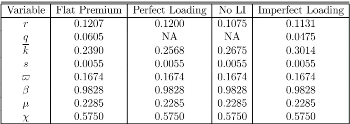
We first examine the results of our moment-matching calibration exercise under a constant premium (Flat Premium) over all ages. These results are presented in Table 12. As can be seen, the interest rate r−δ is around
2 percent per annum which is a reasonable value for risk-free government debt over the postwar US period. However, this value is about around half the average return to capital measured from NIPA data in McGrattan and Prescott (2003). Given that we have abstracted from default and aggregate risk, we do not find this to be a failure of the model.
More relevant for our investigation are the values for q, k, and s. The life insurance premium is quite high relative to the death probability for young households — we plot the mortality rates for a household, for a male and for a female in Figure 6. The equilibrium price is0.0605, which exceeds the mortality rate for households, males or females under (model) age 45. At this price, the young household is getting a particularly bad deal on life insurance. Because life insurance is expensive, the holding of life insurance is restricted to older households; these households pay relatively low premiums and expect to get a payout with a high probability. This is seen very clearly in upper part of Figure 7. The hump to the right, which begins around age 55, represents the holding of life insurance generated by the model under this pricing strategy. Using the axis on the right hand side, we can see that the amount of life insurance holding is small. Another way to judge the model is to compare life insurance holdings relative to GDP. According to actual data, the combined amount of life insurance — term plus the non-cash value portion of whole-life — is around110 percent of GDP in 1998. In our model economy with a constant premium, we observe that total life insurance holdings is approximately 4 percent of GDP. The amount of capital held by singles,k, is quite low; they hold about 13 percent of the total wealth in the economy, suggesting that life insurance may be critical for mitigating the effects of martial risk. Finally, the accidental bequest term is small; this term matters
in this environment because it acts like free insurance and we do not want it to contaminate our results.
Within this economy, we examine certain demographic subsamples of the population. One of the main issues in the empirical literature has been the wealth of new widows. Bernheim et.al. (2001a,2001b) suggest that household members do not carry enough life insurance to protect themselves against a permanent and sizable drop in their consumption. In our model, we can compute the change in lifetime resources — defined as the expected future value of labor income plus government transfers plus current financial wealth — caused by the loss of a spouse at various points in the distribution. To get at this, we measure the wealth difference generated by being a widow instead of being married. The average wealth of a widow is substantially less than a married household. The average wealth of a married household is1.82
while the average wealth of a widow is 1.29. Since very little life insurance is being purchased, the widows are not being protected from early death of their spouse.
We need to adjust the pricing mechanism so that we get premiums which are more actuarially-fair for the working age household. We will consider a pricing strategy where each household pays a premium exactly equal to the probability that an adult member will die. We will refer to this pricing strat-egy as perfect loading. Now cross-subsidization over ages does not occur.25
Under this pricing policy, the model generated holdings of life insurance changes drastically from the constant premium case. Younger households purchase life insurance as the premiums are much lower than the previously examined pricing policy. In upper part of Figure 7, we plot the distribution of life insurance holdings by age. As can be seen, life insurance holding begin to occur at model age 4 and peak around model age 25. Individuals older than model age 45 do not hold life insurance. This ”hump-shaped” pattern of life insurance is consistent with what we observed in actual data, although somewhat more pronounced. It is also important to note that the peak of life insurance holdings occurs before the peak in earnings. This matches with previously documented observations from the data and is consistent with the 25One caveat to note about our computations here is that the sampling error introduced
by our Monte Carlo approach to calculating the transition matrix is no longer innocuous. Since each household will pay the premium equal to their probability of loss, small irregu-larities in the mortality rates generate large irreguirregu-larities in life insurance holdings. Thus, we are careful to generate death probabilities which match the observed data.That is, the small dip in the death probability of males around age 30 is actually observed in the data.
idea that life insurance is a hedging vehicle for risk to the uncapitalized hu-man wealth that younger households have in abundance. In effect, since the premium is low households ”borrow” against that future income by reducing their precautionary savings, using the state-contingent payout of life insur-ance to protect themselves. In fact, the peak in holdings is consistent with the peak in the present value of future income.
Another way to evaluate the model is to calculate the life insurance-GDP ratio. We now observe that life insurance holdings are 95 percent of GDP. This ratio is much closer to the observed value. In our model economy, single individual households have no motivation for buying life insurance. Yet, we do observe some life insurance holdings in thr data. Since only married households would life insurance in our model economy, we also calculated the ratio of married household life insurance holdings to GDP. The actual ratio is 0.64 which is smaller than that produced by the model. Overstating the purchases of life insurance is to be expected since adverse selection problems will typically create actuarial unfairness for some members of society.
We now want to address the potential puzzle that single earner mar-ried households have a lower life insurance participation rate than do dual earner married households. We find that 72.2 percent of single earner mar-ried households have life insurance while 75.4 percent of dual earners hold life insurance. The high risk households are participating less in life insur-ance just as in the observed data. At first glance, it would appear that this feature is not a puzzle. However, the data shows that on average the single earner and dual earner households have roughly the same wealth, while the model does not replicate this observation. The average wealth of dual earner households is 1.70, while the average wealth of a single earner household is
0.93. Thus, part of the answer for the high life insurance participation rate that we observe ifor dual earners is the wealth effect; wealthier household participate more in the life insurance market. Since dual earner households have more wealth, we should expect a boost in their life insurance partici-pation. Thus, we have not yet established whether the participation rate should be considered a puzzle.
Since young households are now purchasing life insurance, we should see how the wealth of widows compares with married households. We find that average wealth for widows is1.15. This is quite a bit lower than the average wealth of married households which is 1.70. It appears that widows still suffer large wealth losses. However,when we compare working age widows with working age households, we find a different story. Widows, on average,