Monte Carlo convolution for learning on non-uniformly sampled point clouds

for Learning on Non-Uniformly Sampled Point Clouds

PEDRO HERMOSILLA,

TOBIAS RITSCHEL,

PERE-PAU VÁZQUEZ and ÀLVAR VINACUA,

TIMO ROPINSKI,

Continuous ground truth Uniform sampling Non-uniform sampling

Previous Non-uniform samplingOurs

Space Value Space Value Input O utput Space Value Space Value Space Value Space Value Space Value Space Value Real da tar esult

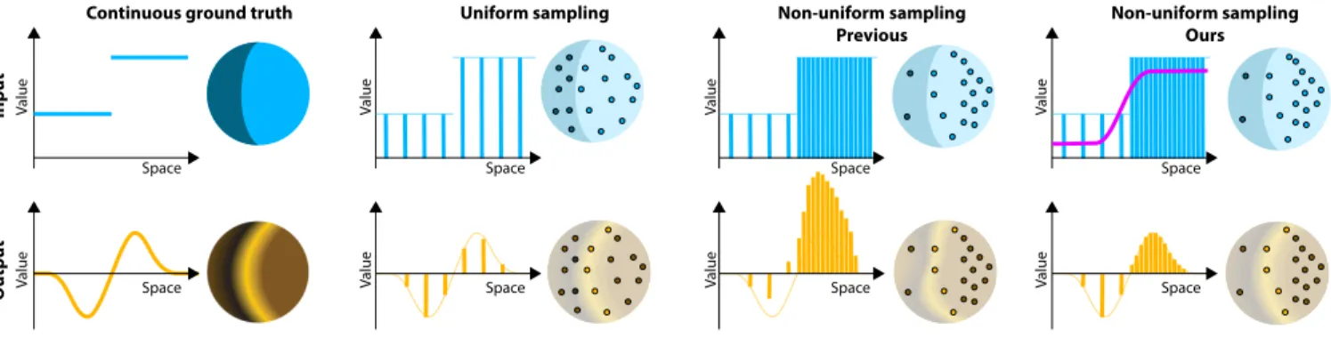
Fig. 1.Non-uniform sampling, which is inherent to most real-world point cloud datasets, has a severe impact on the convolved result signal. An input signal represented as 1D function and as projected on a 3D sphere_{(top row)}is convolved with an edge-detection kernel to obtain the output signal represented as 1D function and as projected on a 3D sphere_{(bottom row)}. The four columns illustrate the impact of the sample distribution on the convolution result. The ground truth continuous signal’s filter response_{(first column)}is faithfully captured when convolving uniformly sampled point clouds_{(second column)}. In the case of non-uniformly sampled point clouds, state-of-the-art convolutional methods severely deviate from the desired filter response(third column). With our interpretation of non-uniform convolution as a Monte Carlo estimate in respect to a given sample density distribution (illustrated by the pink line), we can compensate this deviation and obtain a filter response faithfully capturing that of the ground truth(fourth column).

Deep learning systems extensively use convolution operations to process

input data. Though convolution is clearly defined for structured data such

as 2D images or 3D volumes, this is not true for other data types such as

sparse point clouds. Previous techniques have developed approximations to

convolutions for restricted conditions. Unfortunately, their applicability is

limited and cannot be used for general point clouds. We propose an efficient

and effective method to learn convolutions for non-uniformly sampled point

clouds, as they are obtained with modern acquisition techniques. Learning

is enabled by four key novelties: first, representing the convolution kernel

itself as a multilayer perceptron; second, phrasing convolution as a Monte

Carlo integration problem, third, using this notion to combine information

from multiple samplings at different levels; and fourth using Poisson disk

sampling as a scalable means of hierarchical point cloud learning. The key

idea across all these contributions is to guarantee adequate consideration of

the underlying non-uniform sample distribution function from a Monte Carlo

perspective. To make the proposed concepts applicable to real-world tasks,

Authors’ addresses: Pedro Hermosilla, Ulm University, Germany, pedro- 1. hermosilla- casajus@uni- ulm.de; Tobias Ritschel, University College London, United Kingdom, [email protected]; Pere-Pau Vázquez, [email protected]; Àlvar Vinacua, [email protected], Universitat Politècnica de Catalunya, Spain; Timo Ropinski, Ulm University, Germany, timo.ropinski@uni- ulm.de.

Permission to make digital or hard copies of part or all of this work for personal or classroom use is granted without fee provided that copies are not made or distributed for profit or commercial advantage and that copies bear this notice and the full citation on the first page. Copyrights for third-party components of this work must be honored. For all other uses, contact the owner /author(s).

© 2018 Copyright held by the owner/author(s). 0730-0301/2018/11-ART235

https://doi.org/10.1145/3272127.3275110

we furthermore propose an efficient implementation which significantly

reduces the GP U memory required during the training process. By employing

our method in hierarchical network architectures we can outperform most

of the state-of-the-art networks on established point cloud segmentation,

classification and normal estimation benchmarks. Furthermore, in contrast to

most existing approaches, we also demonstrate the robustness of our method

with respect to sampling variations, even when training with uniformly

sampled data only. To support the direct application of these concepts,

we provide a ready-to-use TensorFlow implementation of these layers at

https://github.com/viscom- ulm/MCCNN.

CCS Concepts: •Computing methodologies→Neural networks;Shape

analysis;

Additional Key Words and Phrases: Deep learning; Convolutional neural

networks; Point clouds; Monte Carlo integration

ACM Reference Format:

Pedro Hermosilla, Tobias Ritschel, Pere-Pau Vázquez, Àlvar Vinacua, and Timo

Ropinski. 2018. Monte Carlo Convolution for Learning on Non-Uniformly

Sampled Point Clouds.ACM Trans. Graph.37, 6, Article 235 (November 2018), 12 pages. https://doi.org/10.1145/3272127.3275110

1 INTRODUCTION

While convolutional neural networks have achieved unprecedented performance when learning on structured data [He et al. 2015; Huang et al. 2016; Wang et al. 2017], their application to unstruc-tured data such as point clouds is still fairly new. Early methods have looked into fully-connected approaches and striven for permutation

and rotational invariance [Guerrero et al. 2018; Qi et al. 2017a,b]. Unfortunately, a non-uniform sampling typically associated with real-world point cloud data, such as for instance resulting from the projective effect of a LiDAR scan, has not been a special focus of previous research. As the underlying sampling results in severe im-plications, as illustrated in Fig. 1, we propose a new approach which has been developed with a special focus on non-uniformly sampled point clouds, achieving at the same time competitive performance on uniformly sampled data.

To make progress towards our goals, we take into account the original definition of convolution: an integral in an unstructured setting. By using Monte Carlo (MC) estimation of this integral, we will show that proper handling of the underlying sampling density is crucial, and will produce results surpassing the state-of-the-art.To this end, we make four key contributions.

First, we represent the convolution kernel itself as a multilayer perceptron (MLP). Since a convolution kernel maps a spatial off-set (Laplacian) to a scalar weight, representing and learning this mapping through an MLP is a natural choice.

Second, we suggest using Monte Carlo integration to compute convolutions on unstructured data. Key is the adequate handling of the non-uniformity and varying-density of points from a Monte Carlo point of view. Averaging weighted pairs of points formally means to sample an MC estimate of an integrand. While MC requires to divide by the probability of each sample, this can be neglected in a uniform setting, as it would result in a division by a constant. However, when dealing with a varying sample density as present in non-uniformly sampled point clouds, failing to perform this nor-malization leads to a bias and consequently reduced learning ability. Therefore, we claim that our approach provides a new form of ro-bustsampling invariance, where for instance simply duplicating a point will not change the estimated integrand. Stating convolution as MC integration allows us to tap into the rich machinery of MC including (quasi) randomization [Niederreiter 1992] and importance sampling [Kahn and Marshall 1953]. Consequently, the convolution becomes invariant under point re-orderings and typically works on receptive fields with a variable number of neighboring points.

Third, we show how this allows generalizing convolutions which use a single sampling pattern to convolutions that map from one sampling pattern to a different one with a higher or lower reso-lution. This can be used to learn (transposed) convolutions that change the level-of-detail for pooling or up-sampling operations. Even more general, we introduce convolutions that map from mul-tiple input samplings to the desired output sampling allowing to learn combining information from multiple scales.

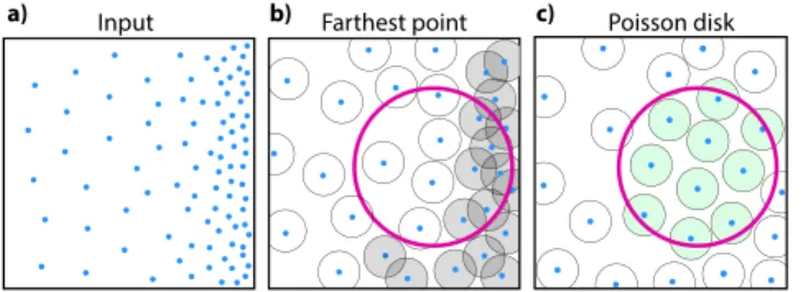
Fourth, we introduce Poisson disk sampling [Cook 1986; Wei 2008] as a means to construct a point hierarchy. It has favorable scalability compared to the state-of-the-art Farthest Point [Eldar et al. 1997] sampling and allows to bound the maximal number of samples in a receptive field.

The usefulness of these novelties is demonstrated by comparing our approach to state-of-the-art point cloud learning techniques for segmentation, classification, and normal estimation tasks. We will show that we outperform the state-of-the-art when learning on non-uniform point clouds, while we still achieve state-of-the-art performance for uniformly sampled point clouds.

2 PREVIOUS WORK

A straight-forward method to enable learning on point clouds is to resample them to a regular grid and then applying learning ap-proaches originally developed for structured data. While extensions to multiple resolutions exist, e. g., based on octrees [Wang et al. 2017], in this section, we will solely focus on those techniques which enable learning directly on unstructured data.

PointNet [Qi et al. 2017a] pioneered deep learning on unstruc-tured datasets. It used a fully-connected network together with a clever machinery to achieve rotation and permutation-invariance. PointNet++ [Qi et al. 2017b] added extensions to support localized sub-networks, but was not yet fully convolutional. PCP Net [Guer-rero et al. 2018] allowed the inference of local properties like curva-ture or normals but was also not convolutional.

Klokov and Lempitsky [2017] presented a convolutional learner which used ak-d tree. However, since the leaf nodes of the tree had a fixed number of points, it was sensitive to varying density, being tight to the logic of building and queryingk-d trees. In contrast, our approach uses a regular grid to access neighbors in constant time and thus works on multiple scales.

Shen et al. [2017] also provided a translation-invariant but non-convolutional method, where convolution was replaced with the correlation of local neighborhood graphs and learned graph tem-plates. While showing good performance on small problems, it remained particularly sensitive to the underlying graph structure. Dynamic Graph CNNs by Wang [2018] were convolutional. They employed a general notion of learnable operations on edges of a graph of neighboring points. In contrast to other approaches, they changed neighborhoods during learning, making the approach slightly more complex to implement and less efficient on large point clouds.

PointCNN [Li et al. 2018] was also convolutional, working on the

knearest neighbors. They used an MLP on the entire neighborhood to learn a transformation matrix which was used later to weight and permute the input features of the neighboring points. Then, a standard image convolution was applied to the transformed features. SPLATNet [Su et al. 2018] sought inspiration from the permutohe-dral lattice [Adams et al. 2010] where convolutions can efficiently be performed on sparse data in high dimensions while the filter kernels are discrete masks in lattice space. Uneven sample distributions in the lattice are addressed by “convolving the 1” [Adams et al. 2010] i. e., repeating the convolution on a unit signal. Our work achieves the same, but without the complication of creating a lattice.

Atzmon et al. [2018] use radial basis functions defined on a dis-crete set of points to represent convolution kernels. The work is computationally demanding but provides invariance under global uniform resampling by construction. However, non-uniform sam-pling settings are not considered.

In concurrent work, SpiderCNN [Xu et al. 2018] used step func-tions to represent convolufunc-tions. The authors mentioned using MLPs, as we do as well, but found them to perform worse than step func-tions. Nevertheless, in our architectures, we found MLPs to perform well. We acknowledge that further work shall explore different continuous representations to parametrize learned convolutions.

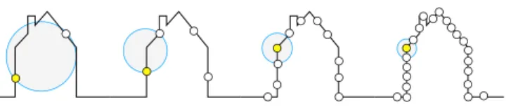
Fig. 2. Ak =2-nearest neighbor receptive field(blue circle)in a scene with non-uniform sampling of the same house-like geometry changes scale.

Groh et al. [2018] suggested using a linear function as a represen-tation of an unstructured convolution kernel. With considerations how dissimilar 2D convolution kernels are from linear functions, we think an MLP to describe a kernel is worth exploring. Thanks to the simplicity we share in our approach, they demonstrated excellent scalability to millions of points, but the problem of non-uniform sampling is not touched upon.

Most of the existing methods are based on convolving thek near-est neighbors (using a hierarchical structure or not) [Groh et al. 2018; Klokov and Lempitsky 2017; Li et al. 2018; Shen et al. 2017; Wang et al. 2018; Xu et al. 2018]. This approach is not robust in non-uniform sampling settings, since adding more points into a region in the space will reduce theknearest neighbors to a small volume around each point, capturing different features from those the kernel was trained on, i. e. it shrinks in densely populated areas and grows in sparse ones. We see in Fig. 2 how this would prevent constructing a sampling-invariant “house detector”. Aztmon et al. [2018], although not considering non-uniformity in their paper, transform the point cloud to volumetric functions which can be robust to non-uniformly sampled point clouds. However, some com-putations of their method are quadratic on the number of points which makes their method not scalable. PointNet++ [Qi et al. 2017b], on the other hand, computes features locally, which makes it scal-able. Moreover, it was tested with non-uniformly sampled point clouds by simulating the properties of LIDAR scans. Nevertheless, their method selects a fixed number of random samples within a radius around the points and thus does not consider the point den-sity in its computations, which, as we will demonstrate, can lead to errors.

3 CONVOLUTION KERNELS

Here, we will first recall the definition of a convolution (Sec. 3.1). Then, we will introduce a kernel representation using MLPs (Sec. 3.2) which shall allow efficient and simple learning on irregular data.

3.1 Convolution as an integral

Recall the definition of a convolution as an integral of a product:

(f ∗д)(x)=

∫

f(y)д(x−y)dy (1)

where f is a scalar function on_R3to be convolved andдis the

convolution kernel, a scalar function on_R3. In our particular case,f is thefeature functionfor which we have a setSof discrete samples xi ∈ S (our data points). If for each point no other information is provided besides its spatial coordinates,f represents the binary function which evaluates to 1 at the sampled surface and 0 otherwise. However,f can represent any type of input information such as

x y x y x y z

g1 g1 g2 g1 g2 g3 g4 g5 g6 g7 g8

a) b) c)

Fig. 3. Evolution of MLP kernels:a)A naïve solution would map one 2D offsetx,y(blue dots) to one scalar resultд(orange dots).b)We sug-gest extending this to multiple outputs, e. g.,д1andд2, which speeds up

computation and reduces the number of learnable parameters.c)Our 3D implementation uses two hidden layers of 8 neurons outputting 8 kernel values. In this example we require2×8×8+3×8=152operations to learn and compute while a naïve approach needs8× (3×8+8×8+8)=768.

color, normals, etc. For internal convolutions, i. e., those which are subsequent to the input layer, it can also represent features from a previous convolution.

Translation-invariance. As the value ofдonly depends on relative positions, convolution is translation-invariant.

Scale-invariance.Since evaluating the integral in Eq. 1 over the entire domain can be prohibitive for large datasets, we limit the domain ofдto a sphere centered at 0 and radius 1. In order to support multiple radii, we normalize the input ofдdividing it by the receptive fieldr. In particular, we chooserto be a fraction of the scene bounding box diameterb, for instancer=.01·b. Doing so results in scale-invariance. Note, that this construction results in compactly-supported kernels that are fast to evaluate.

Rotation-invariance.Note, that we do not achieve and seek to achieve rotation-invariance. Typical image convolutions are not rotation invariant either and succeed nonetheless.

3.2 Multilayer perceptron kernels

We suggest to represent the kernelд, by a multilayer perceptron.

Definition.The multilayer perceptron (MLP) takes as input the spatial offsetδ =(x−y)/rcomprising of three coordinates, normal-ized dividing them by the receptive fieldr. The output of the MLP is a single scalar. To balance accuracy and performance, we use two hidden layers of 8 neurons each (see Sec. 8 for more details). We denote the hidden parameters as a vectorω.

For layers with a high number of input and output features, the number of kernels and therefore the number of parameters the network has to learn is too high (#inputs×#outputs). To address this problem, we use the same MLP to output 8 differentд’s, thus reducing the number of MLP’s by a factor of 8. Fig. 3 presents an illustration of such an MLP, which takes three coordinates as input and outputs 8 differentд’s.

Back-propagation. For back-propagation [Rumelhart et al. 1986], the derivative of a convolution with respect to the parameterω_lof the MLP is δ f ∗д δω_l = ∫ f(y)δд(x−y) δω_l dy. (2)

x r

p(_yj|x) yj

a) b) c) d)

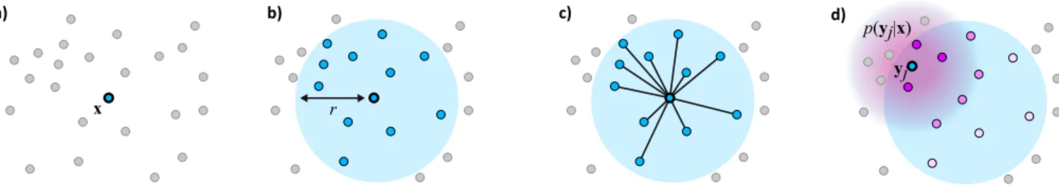
Fig. 4.Steps of our MC convolution. For a given pointx_(a)the neighbors within the receptive fieldrare retrieved_(b)to be used as Monte Carlo integration samples(c). For each neighboring pointy_j, its probability density function,p(y_j|x), is computed usingKernel Density Estimation[Parzen 1962; Rosenblatt 1956](d). Based on the bandwidth used (pink disk), the neighboring points have different effects on the computation ofp(y_j|x)(pink gradient).

3.3 Single- and multi-feature convolution

Our convolution consumesMinput feature functions and outputsL convolved feature functions. Based on the way the convolved feature functions are calculated, we define two types of layers:Single-feature spatial convolution andMulti-featurespatial convolution. Single-feature spatial convolution outputs a scalar Single-feature by convolving a scalar input feature. Therefore, in these layers, the number of output features is equal to the number of input features,M =L, and the number of kernelsдis also equal toM. The multi-feature convolution, on the contrary, is similar to the layers used in stan-dard convolutional neural networks where each output feature is computed as the sum of all input feature functions convolved:

fo = M

Õ

i=0

fi∗дo,i (3)

These layers are more computationally demanding since they have to learnM×Lconvolution kernelsд.

4 MONTE CARLO CONVOLUTION

In this section, we will show how convolutions can be stated as a Monte Carlo estimate by relying on a sample’s density function, which ultimately makes learning robust to non-uniform sample distributions.

4.1 Monte Carlo integration

In order to compute the convolution in each sample point, we have to evaluate the integral of Equation 1. Since we only have a set of samples of our functionf, we propose to compute this integral by using MC integration [Kalos and Whitlock 1986], which uses a set of random samples to compute the value of an integral.

Definition.In our case, these samples comprise of the input data points or a (quasi) random subset. Therefore, an estimate of the convolution for a pointxis

(f ∗д)(x) ≈ 1 |N(x)| Õ j∈N(x) f(yj)дx−yj r p(yj|x) , (4)

whereN(x)is the set of neighborhood indices in a sphere of radius

r (the receptive field), andp(y_j|x)is the value of theProbability

Density Function(PDF) at pointy_j when the pointxis fixed, i. e.,

the convolution is computed atx. Fig. 4 provides an illustration of this computation.

Please note that, since our input data points are non-uniformly distributed, each pointy_jwill have a different value forp(y_j|x). It is also worth noticing, that the PDF depends not only on the sample positionyjbut also onx: How likely it is to draw a point does not only depend on the point itself, it also depends on how likely the others in the receptive fieldrare.

Please finally note that, here and in the following,xis an arbitrary output point that might not be from the set of all input pointsy_j. This property will later allow re-sampling to other levels or other irregular or regular domains.

Back-propagation. Back-propagation [Rumelhart et al. 1986] with respect to the MLP parametersω_lcan also be estimated using MC:

_{δ f} ∗д δω_l (x)= 1 |N(x)| Õ j∈N(x) f(yj) p(yj|x) δд_x−y j r δω_l . (5) 4.2 Estimating the PDF

Unfortunately, the sample density itself is not given but must be estimated from the samples themselves. To do so, we employ Kernel Density Estimation [Parzen 1962; Rosenblatt 1956]. The function estimated is high where the samples are dense and low where they are sparse. It is computed as

p(yj|x) ≈ 1 |N(x)|σ3 Õ k∈N(x) ( 3 Ö d=1 h _y j,d−yk,d σ ) , (6)

whereσis the bandwidth which determines the smoothing of the resulting sample density function (we useσ =.25r),his the Density Estimation Kernel, a non-negative function whose integral equals 1 (we use a Gaussian), anddis one of the three dimensions of_R3.

The PDF of a pointy_jin respect to a given pointxis always rela-tive to all other samples in the receprela-tive field. Therefore, density can not be pre-computed for a pointy_jsince its value will be different for each receptive field defined byxand radiusr. Note that in a uniform sampling settingpwould be a constant.

5 MC CONVOLUTION ON MULTIPLE SAMPLINGS

Our construction does not only allow handling varying sampling densities but also to perform convolution between two (Sec. 5.1) or even multiple different samplings (Sec. 5.2).

*

*

*

*

*

*

Same Sampling Different

M ultiple Single Fea tur es

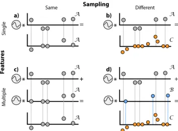
Fig. 5. Monte Carlo convolution for the same / different sampling

(hor-izontal)and a single / multiple feature channels(vertical). Samples are denoted as dots, whereby lines indicate if samplings match. Colors indicate the samplingsA,BandC.

Convolution involving a single sampling is illustrated in Fig. 5 (a). Here, the samplingAof the input and the output is identical. While the previous section has detailed how to account for varying sampling density, we will show in this section how MC convolution can seamlessly handle two or more samplings.

5.1 Two samplings

A more generalized setting is shown in Fig. 5 (b). Here, the input sampling is stillA, but the output is on a different samplingC.

The illustration shows a mapping from a lower sampling to a higher sampling (also called upsampling, transposed convolution or deconvolution). The same principle can be used to reduce the sample resolution (pooling), as necessary for example when an entire point cloud is successively reduced in resolution to produce a single scalar classification value. We will make use of combinations of up- and downsampling in a U-net / encoder-decoder architecture [Ronneberger et al. 2015] for our segmentation application.

Previous work also operated using different samplings in a multi-resolution hierarchy, but using fixed, non-learned interpolation, e. g., inverse-distance weighting [Qi et al. 2017b] for upsampling operations. Our approach allows learning these mappings instead. The procedure explained in the previous section simply works in the two-sampling case, as the kernelsдare defined on all continuous offset vectorsxC−yA, that can be computed at any output position xCin samplingC, and input positiony_jAin samplingA. Note, that a density estimation has to be performed respectively toA, the input, as explained in the previous section.

5.2 Multiple samplings

Another unique advantage of our construction is to relax the sam-pling requirements not only between the input and output samsam-pling

AandC, but also between the different inputs. The case of multiple input channels is seen in Fig. 5 (c) and (d). For Fig. 5 (c) the sampling remains identical (A) between two input channels and the output.

Layer i-2 Layer i-1 Layer i x f_i-2 p_i-2 f_i-1 p_i-1 g_i-2 g_i-1 f_i(x)

Fig. 6. Features upsampled from different levels for a single black pointx on layeriwith respect to two previous layers. The receptive field content

fi−1andfi−2is shown on the right, with their respective densitiespi−1and

pi−2in pink. Each layer is MC-convolved using an individual MLP kernel

дi−1andд_i−2which results are concatenated to create the feature vector

for pointxof layeri. We guarantee the same maximum number of points in all receptive fields by maintaining the same ratio between the Poisson disk and the radius of the convolutions.

In Fig. 5 (d) the sampling is mutually different between both inputs and the output.

A typical application of this multiple-sampling approach is to consume information from multiple resolutions in a hierarchy at the same time. Our example shows a learned up-sampling from five samples atAand three samples at levelBwhich are combined into a ten-sample resultC. Note, that in the multiple-samplings case, density estimation is to be performed relative toAwhen convolving samples fromAand relative toBwhen processing points fromB. Combining output from multiple previous layers has also been used in DenseNet [Huang et al. 2016], but the classic tabulated kernels do not admit to construct dense links between different samplings.

We are not limited to use the same receptive field size on all samplings but each can choose its own, such that the number of samples falling into the receptive field remains roughly constant. Note, that any deviation from this desired constant sample count, as well as variation of density inside the receptive field, is compensated for using the density estimation.

A particular embodiment of multi-sampling MC convolution is shown in Fig. 6, where information from two 2D point clouds with different resolutions are up-sampled into a third one with a higher resolution. Note how the receptive field grows in the level with a lower resolution.

6 POISSON DISK HIERARCHY

Deep image processing routinely reduces – and later increases again – the image resolution to make use of both local and global informa-tion. The same is achieved in deep point cloud processing [Qi et al.

Table 1. Time for sampling a tenth of the points using different algorithms.

100/1 k 1 k/10 k 10 k/100 k 100 k/1000 k

Poisson disk 10.4 ms 21.7 ms 136.4 ms 1,304.9 ms

Farthest Point 2.4 ms 11.9 ms 657.1 ms 108,682.8 ms

2017a] usually using Farthest Point (FP) sampling [Eldar et al. 1997]. In this work, we favor using Poisson disk (PD) sampling [Cook 1986] instead. This has two reasons: scalability and the ability to preserve the sampling pattern while bounding the sample count per unit measure.

Realization. PD is realized as a network layer using the Parallel Poisson Disk Sampling algorithm [Wei 2008]. The input for these layers are any point sampling and a parameterrpcontrolling the PD radius. The output is a sampling with a minimum distance between points equal torp. Note that this does not bound the distance from above, so areas with distances much larger thanrpcan remain.

Multiple PD layers can be combined to create a multi-resolution hierarchy. We use this in combination with multi-samplings convo-lution (Sec. 5) to build an encoder-decoder network [Ronneberger et al. 2015] for point clouds.

Note that, contrary to other sampling approaches, this technique generates a non-fixed number of samples. Therefore, our networks cannot take advantage of acceleration techniques commonly used by deep learning frameworks in which the memory required for a forward pass is reserved in advance. However, we still achieve good performance as is presented in Section 8.7.

Scalability.The main practical reason to use PD is scalability to large point clouds as evaluated in Tbl. 1. We see, that PD sampling presents a low compute time for the different model sizes (linear to the number of points in the model). FP sampling, on the other hand, does not scale well, requiring more than 100 seconds to sample 100 k points from a 1,000 k points model.

Sample count bound.Moreover, PD allows us to limit the number of points within the receptive fields of our convolutions. The Ke-pler conjecture [Hales et al. 2017], provides an upper bound to the number of points inside the receptive fields: This is illustrated in Fig. 7. Starting from a non-uniform sampling(a), PD will retain non-uniformity whilst maintaining a minimal distance between points

(c). Therefore, any ball, such as the receptive field of our approach (pink circle) will at most retain a bound number

n<π r+rp 2 3 3 √ 2rp 3 , when rp⩽r,

of balls of the Poisson disk radiusrp(marked in green) in a receptive field of radiusr.

In practice, the number of points is much lower than this limit since we learn from points sampled on the surface of a 3D object. As it is illustrated in Figure 6, we can take advantage of this fact to compute features at different scales by maintaining a constant ratio betweenrandrp. We found that a ratio between 4 and 8 provides enough samples in our receptive fields (∼30).

c)

a) _Input b) _{Farthest point Poisson disk}

Fig. 7. Result of Farthest Point (FP) (selecting a fix number of samples) and Poisson Disk (PD) sampling for non-uniformly sampled inputs. Blue dots are samples, the pink circle denotes the receptive field. Grey circles in FP (b) are samples not fulfilling a minimal distance (overlap). Green circles in PD (c) are balls around samples that can be packed inside the receptive field.

The most commonly used implementation of FP sampling [Qi et al. 2017a] for learning on point clouds, selects a fixed number of samples from the input point cloud. Contrary to PD, this method cannot bound the number of points that fall in the receptive fields

(b). In order to generate a sampling with the same properties as PD, this method would need to be modified to select a variable number of points based on the distance of each new sample to the subset of already selected ones.

7 IMPLEMENTATION

In this section, we describe several implementation details of the building blocks of the proposed learning approach.

PDF computation. Our implementation differs from averaging

the individual contributions of the neighboring points only by the requirement to divide by their probability valuesp. Therefore, our MC approach requires two steps: computing all values ofpand querying them during MC convolution.

To computep, we create a voxel grid with cell sizer, as in [Green 2008], which enables us to perform the desired computation in time and space linear wrt. the number of points. Further scalability would be provided using hashing instead of a regular grid as proposed by Teschner et al. [2003].

For lookup performance, the neighbor indicesN(x)of all points xare stored in a flat list, which is indexed by a start and end index stored at each grid cell. Additionally, we compute the values of

p(yj|x) and store them in a list of the same size. Both lists can get arbitrarily long with arbitrarily high density, which decreases performance during the computation of our convolution for large values ofr. However, maintaining a good ratio between the receptive field and the PD radius provides an upper bound on the number of neighbors of each point.

Based on the thus constructed data structures, the neighbor in-dices, as well as the precomputed PDF, can now be looked-up in constant time using the computed information. When looking up the neighbor values, they are multiplied by the kernel weight

д((x−yj)/r)and divided by thep(y_j|x).

Note that the voxel grid in which points are distributed is com-puted in parallel on the GP U, resulting in different point orderings within the same cell for different executions. This introduces ran-domness in the output sampled point clouds of our PD sampling

strategy, which is preferred during learning. Sec. 8 evaluates the effect of the randomness on the resulting accuracy.

Multilayer Perceptron Evaluation.Evaluating the MLP during MC convolutions requires a considerable amount of GP U memory when using implementations as provided by standard frameworks. This limits the number of computed features per point and the number of convolutions used in the network architecture. In order to address these limitations, we have implemented the MLP evaluation in a single GP U kernel. By doing so, our networks do not require to expand the features and coordinates of neighboring points and also do not need to store intermediate MLP results for each layer. However, with this implementation, we are not able to use some features, such as batch normalization, to improve learning.

Batch Processing.Our layers process point clouds of variable size. Moreover, as described in Section 4, our convolutions take into account all the neighboring points to carry out their computations. These design choices do not allow us to use the standard tensor approach to process a batch of models in parallel.

In order to support batch processing, we use an extra vector with an integer value for each point, denoting the model identifier to which the point belongs to. We create an acceleration data structure to access neighboring points (as described at the beginning of this section) for each model, and, during the evaluation of the layers, only the appropriate data structure is updated and queried based on the model identifier of each point. This simple approach allows us to process batches of models with variable size in parallel by increasing the memory consumption linearly with the number of points. However, in configurations with reduced GP U memory, a more sophisticated approach can be considered, such as only storing the number of points per model and perform extra computations within the layers.

8 EVALUATION

Here we report the results obtained when using the machinery explained before in a complete network on specific data for relevant tasks. To make the reported results comparable, we introduce a dataset with non-uniform sampling in Sec. 8.1 based on current benchmark data. Next, we describe the specific tasks carried out in Sec. 8.2 and the methods used in Sec. 8.3, before reporting actual quantitative evaluation results in Sec. 8.4. Moreover, we report the results of applying our networks to process real-world datasets in Sec. 8.5. And, lastly, we introduce additional experiments in Sec. 8.6 and present the computational efficiency of our networks in Sec. 8.7.

8.1 Non-uniformly sampled test data

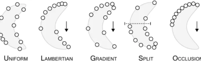
Non-uniform test data is found in typical scanned scenes. How-ever, existing benchmarks provide data sets of uniformly sampled models [Wu et al. 2015; Yi et al. 2016]. In order to evaluate the per-formance of our and other state-of-the-art networks, we generated our own data set by artificially producing non-uniform samplings (see Fig. 8). This allows us to explicitly study the effect of sampling. To produce such data, we start from a uniformly sampled point cloud, and at each point perform rejection sampling, whereby the rejection probability is computed according to one of five protocols:

UNIFORM LAMBERTIAN GRADIENT SPLIT OCCLUSION Fig. 8.Different sampling protocols applied to the same object. Uniform is uniformly random. Lambertian depends on the orientation, here shown as an arrow. Locations facing this direction are more likely to contain points. For Gradient, the likelihood of generating a point decreases along a direction, here shown as an arrow again. For Split, the shape is split into two halves, here shown as a dotted line, where each part is samples uniformly random, but with different density. Occlusion also depends on the orientation. Only locations visible from this direction contain points.

Uniform (no rejection), Split (probability is either a random con-stant smaller than 1 in a random half-space or 1, we used 0.25 in our tests), Gradient (probability is proportional to the projection onto the largest bounding box axis), Lambertian (probability is propor-tional to the clamped dot product between the surface normal and a fixed “view” direction) and Occlusion where probability is one except for points invisible from a certain direction. These sampling protocols are applied during the training and testing phase on the data sets of the different benchmarks. Thus, each time a model is loaded, we apply one of these sampling techniques (the one we are currently testing) with a random seed to generate the probabilities of each point and the view direction where applicable.

8.2 Tasks

In this section, we describe the tasks used to evaluate our networks: classification, segmentation, and normal estimation.

Classification. This task assigns a label to each point cloud as a whole. Its performance is measured in percentage of correct pre-dictions (more is better). We used the resampled version of Model-Net 40 [Wu et al. 2015] provided by Qi et al. [2017a]. This dataset is composed of 12,311 point clouds uniformly sampled from objects of 40 categories. The official split is composed of 9,843 models in the train set and 2,468 in the test set. The models were sampled into 1,024 points according to the different protocols of Sec. 8.1

Segmentation.This task assigns a label to every point. It can be quantified by its intersection-over-union (IoU) metric (more is better). We segment the 16,881 point clouds of ShapeNet [Yi et al. 2016], uniformly sampled from 16 different classes of objects, each one composed of between 2 and 6 parts, making a total of 50 parts. We use the standard train/test split for training [Qi et al. 2017b]. The class of the point cloud is assumed to be known for this task and used as input. We used as input of our networks the complete point clouds, which are in the range of 1,000 to 3,000 points per object.

Normal estimation.This task computes a continuous orientation at every point. It is analyzed by the cosine distance (less is better). Similar to Atzmon et al. [2018], we use ModelNet 40 for evaluation, taking 1,024 points from each model on the standard train/test split.

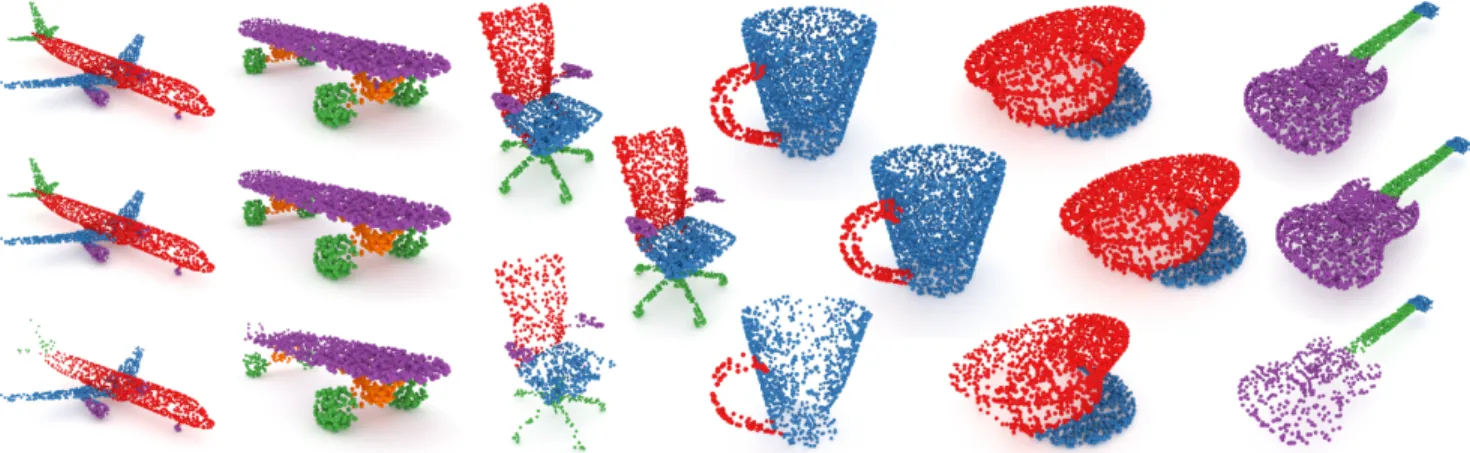
Fig. 9.Comparison of our segmentation result for uniform(second row)and non-uniform samplings(third row)to the ground truth(first row). Non-uniform sampling use the Gradient (first and second columns), Lambert (third and fourth columns), and Split (fifth and sixth columns) protocols.

Table 2. Performance of different methods, including ours,(rows)for dif-ferent tasks(columns)with different measures (please see text).

Classify Segment Normals 1,2 Su et al. [2018] - 85.1 -1 Xu et al. [2018] 92.4% 85.3 -1 Qi et al. [2017b] 91.9 % 85.1 .47 Qi et al. [2017a] 89.2 % 83.7 -Groh et al. [2018] 90.2 % - -Shen et al. [2017] 90.8 % 84.3 -Wang et al. [2018] 92.2 % 85.1 -Li et al. [2018] 91.7 % 86.1 -Atzmon et al. [2018] 92.3 % 85.1 .19 Klokov et al. [2017] 91.8 % 82.3 -MC (Ours) 90.9 % 85.9 .16 1

Additional input 2One network per class in segmentation tasks

8.3 Methods

Please see the Appendix Sec. A for training and network details.

Architecture. A different architecture is used for each task, where we compare three variants: The first is PointNet++ [Qi et al. 2017b] (PN++) with multi-scale grouping (MSG) , serving as a baseline. The second is our own architecture, but without using MC convolution, i. e., kernel-weighted averaging inside the receptive field, denoted as AVG. The last is our architecture using our Monte Carlo convolution (_MC). Additionally, we compare to a range of methods that have reported results for the uniform data we use.

Evaluation.We study two variants of training. The first only trains on uniformly sampled data. The second only on non-uniformly sampled data, i. e., a dataset produced using all sampling protocols from Sec. 8.1 expect Uniform. Then, the trained models are tested on all 5 sampling protocols described in Sec. 8.1. To counterbalance the randomness introduced by the point sampling algorithm, all measurements were averaged across five independent executions.

8.4 Results

Here we discuss the results for uniform and non-uniform sampling as summarized in Tbl. 2 and Tbl. 3, respectively, for every task.

Classification. The results are illustrated in the first column of Tbl. 2. Our approach generates competitive classification results for uniform sampling, achieving 90.9 % of accuracy. More importantly, our networks presented a robust performance on non-uniformly sampled point clouds (see first block of Tbl. 3).

When training only on uniformly sampled point clouds, ourMC method results in better performance than PointNet++ when test-ing on uniformly and most of the non-uniformly sampled point clouds. Our method achieved 90.9 %, 87.6 % and 87.3 % on the Uni-form, Split and Gradient sampling protocols, in contrast to 89.1 %, 84.4 % and 79.7 % achieved by PointNet++. For the Lambert and Oc-clusion protocols, both networks presented a similar performance of around 74−72 %. In this protocol, half the points for each model are missing which makes the task more difficult.

Furthermore, ourMC method presented slightly better perfor-mance than PointNet++ in all protocols when training only on non-uniformly sampled point clouds, achieving between 90.1 % and 90.6 % on the different protocols whilst PointNet++ achieved a per-formance between 89.1 % and 89.8 %.

Lastly, when compared with theAVGnetwork, our MC convolu-tions obtained better performance on all protocols. TheAVGnetwork had more difficulties to generalize, as compared with ourMC net-work, presenting severe over-fitting. In order to prevent over-fitting, we trained theAVGnetwork using the data augmentation strategy followed by PointNet++ [Qi et al. 2017b].

The variance of the resulting accuracy over several executionsMC was.0367, indicating that, the observed mean accuracy is significant.

Segmentation.Results of our method are compared to the ground truth for different models in Fig. 9. The second column of Tbl. 2 presents the performance achieved by our segmentation network on uniform data. These are competitive compared to the state-of-the-art methods, only slightly surpassed by PointCNN [Li et al. 2018]. Our method achieved 85.9 whilst PointCNN achieved 86.1. Please

Table 3. Performance comparison of different methods for three different tasks(columns)for different sampling protocols(rows). For each task, we separate training on “uniform” (left columns) and on “non-uniform” (right columns) data, while test is always done according to a different protocol in each row.

Classification Segmentation Normal estimation

Train→ Uniform Non-Uniform Uniform Non-Uniform Uniform Non-Uniform

Test↓ PN++ AVG MC PN++ MC PN++ AVG MC PN++ MC PN++ AVG MC PN++ MC

Uniform 89.1% 88.3% 90.9% 89.6% 90.1% 83.6 85.6 85.9 84.4 85.2 .469 .165 .161 .623 .377 Split 84.4% 83.3% 87.6% 89.1% 90.6% 82.9 84.9 84.6 84.9 85.7 .581 .220 .204 .595 .222 Gradient 79.7% 82.9% 87.3% 89.3% 90.6% 81.7 83.8 84.0 83.9 85.1 .616 .215 .201 .589 .220 Lambert 74.6% 70.1% 73.0% 89.8% 90.4% 80.7 83.1 82.7 83.8 84.9 1.61 .743 .716 1.33 .221 Occlusion 74.8% 67.9% 72.4% 89.5% 90.2% 81.3 83.4 82.7 84.3 85.5 1.49 .679 .654 1.25 .132 oor wall

unannotated table chair bathtub door sofa shelf sink otherfurniture desk

Fig. 10. Semantic segmentation results of our approach(bottom row)on ScanNet [Dai et al. 2017] compared with ground truth(top row).

note, that PointCNN is based onk-nearest neighbors convolutions, and, as discussed in Section Sec. 2, is not the best approach to handle non-uniformly sampled point clouds.

We state segmentation performance for non-uniform sampling in the middle block of Tbl. 3. When trained only on uniformly sampled point clouds, ourMCnetwork obtained better results on all protocols than PointNet++. Moreover, when trained on only non-uniformly sampled point clouds, although PointNet++ presented a competitive performance, ourMCnetwork also obtained better results than PointNet++ in all protocols.

It is also worth noticing that, as in the classification task, Point-Net++ obtained better results when trained with non-uniformly sampled point clouds. That indicates that the proposed sampling protocols can also be used as a data augmentation technique.

When comparing with theAVGnetwork,MCpresented higher accuracy on the uniformly sampled protocol (MC85.9 vs.AVG85.6) and on the Gradient protocol (_MC84.0 vs._AVG83.8). However,_AVG performed better on the Split (MC84.6 vs.AVG84.9), Lambert (MC 82.7 vs._AVG83.1), and Occlusion protocols (_MC82.7 vs._AVG83.1). Nevertheless, the differences between these networks remain small.

Normal estimation. The results of this task are shown in the last column of Tbl. 2. On uniform data, our network outperformed state

of the art methods, achieving a mean cosine distance of.16 and improving thus the accuracy of.19 reported by Atzmon et al. [2018]. When tested on non-uniform data (see the last block of Tbl. 3), our_MC approach outperforms PointNet++ in all protocols when trained on both uniformly and non-uniformly sampled point clouds. The same network withAVGconvolutions also obtained a good performance. However,MCconvolutions obtained better results.

8.5 Real-world data

We also applied our method to real-world data for a semantic seg-mentation task from ScanNet [Dai et al. 2017]. This dataset is com-posed of 1045 scanned rooms for training, 156 rooms for evaluation, and 312 rooms for testing. The task requires to classify each input point into 20 different categories as shown in Fig. 10.

We report performance as mean per-class voxel accuracy [Dai and Nießner 2018]; a more meaningful measure than the original ScanNet metric (overall voxel accuracy) used on PointNet++. Our approach achieves 62.5 %, in comparison to 60.2 % of PointNet++, 50.8 % of ScanNet, and 54.4 % of the method proposed by Dai and Nießner [2018]. When adding image information from 5 different views, Dai and Nießner achieved 75.0%. Our network is able to gener-ate consistent predictions on unannotgener-ated points and predict correct classes for incorrect annotated objects on the ground truth (door in

Table 4. Classification accuracy and timing for different MLP sizes.

MLP Accuracy Time 4 90.8 % 21.0 ms 8 90.9 % 24.6 ms 16 90.6 % 26.2 ms

Table 5. Train (one epoch) and test time for different tasks.

Train Test Classify 454 s 24.6 ms Segment 2160 s 87.4 ms Normals 426 s 28.1 ms

the second column and sofas in the third column of Fig. 10). These point clouds have up to 600 k points, that our method can handle in 3∼5 seconds during training without splitting it into chunks. 8.6 Variants

Poisson disk hierarchy.In order to evaluate the MC convolutions without considering the Poisson Disk hierarchy, we trained a simple network composed of two convolutions on the normal estimation task. First we trained it usingAVGconvolutions, and then using MCconvolutions. We foundAVGto perform worse thanMCfor uni-form (.305), split (.336) gradient (.334) and lambert protocols (.693). Similarly, the performance ofMCwithout PD was limited for uniform (.282), split (.312) gradient (.310) and lambert (.662) as well. This indicates, that at least for normal estimation, using a PD hierarchy is essential.

MLP size.When comparing the classification accuracy at different MLP sizes (Tbl. 4), the maximal accuracy was obtained at 8 neurons, whilst 4 neurons achieve better timing. We decided to use 8 neurons since it provides the best accuracy-execution time trade-off.

8.7 Computational efficiency

Tbl. 5 presents the time required to train an epoch of our networks and the time required to compute a forward pass for a single model. Training time is measured for one single epoch. Testing time is the time required to process a forward pass of an individual model. Due to our parallel implementation of all the algorithms and our acceler-ation data structures, all networks present competitive performance. The lowest performance is found for the segmentation network since it requires to compute a high number of features for the initial point set. All measurements were used an Nvidia GTX 1080 Ti.

9 LIMITATIONS

Besides the many benefits presented in this paper, the proposed approach is also subject to a few limitations.

The main limitation is that we have to rely on KDE to obtain the PDF, which requires to carefully select the bandwidth parameter to obtain a good PDF approximation. In the future, we would like to further investigate this shortcoming and inspect more advanced PDF estimations, like the selection ofσin KDE using cross-validation, ballooning, or otherwise automate its choice.

While our approach provides an unbiased estimate of the convo-lution – assuming the KDE was reliable – there is a variance-locality trade-off: on one hand, one wants a good locality, small receptive fields and few points in them to allow for fast computation, but these give a noisy estimate. On the other hand, a net with large

receptive fields that contain many points is slower to compute, does not localize, but has less noisy estimates.

10 CONCLUSIONS

We have shown how phrasing convolution as a MC estimate pro-duces results superior to the state-of-the-art in typical learning-based processing of non-uniform point clouds, such as segmenta-tion, classificasegmenta-tion, and normal estimation. This was enabled by representing the convolution kernel itself using a multilayer per-ceptron, by accounting for the sample density function, by using Poisson disk pooling, and by realizing MC up- and down-sampling to preserve the original sample density. Moreover, the experiments demonstrated that our networks are more robust to over-fitting with better generalization, being able to obtain the best performance with-out any data augmentation technique (something mandatory in the classification task if the point density is not considered).

Although other methods were able to present competitive per-formance on some tasks when trained on non-uniformly sampled data, it is not always possible to predict the sampling of our future input data in real-world scenarios. Our model’s ability to generalize and become robust to unseen samplings is of key importance for the success of this type of networks in real-world tasks.

In future work, we would like to apply our idea to inputs of higher dimensionality, such as animated point clouds or point clouds with further attributes, such as color. Another direction for future research could be to consider what a non-uniform density means when dealing with triangular or tetrahedral meshes, that typically do not come with uniform sampling.

ACKNOWLEDGMENTS

We would like to thank the reviewers for their comments. This work was partially funded by the Deutsche Forschungsgemeinschaft DFG) under grant RO 3408/2-1 (ProLint), the Federal Minister for Economic Affairs and Energy BMWi) under grant ZF4483101ED7 (VRReconstruct), TIN2017-88515-C2-1-R (GEN3DLIVE) from the Spanish Ministerio de Economía y Competitividad y 839 FEDER (EU) funds, and a Google Faculty Research Award. We also acknowledge NVIDIA Corporation for donating a Quadro P6000.

REFERENCES

AndrewAdams,JongminBaek,and MyersAbrahamDavis.2010. Fast High-Dimensional Filtering Using the Permutohedral Lattice._{Comp. Graph. Forum (Proc.}

Eurographics)29, 2 (2010), 753–62.

Matan Atzmon, Haggai Maron, and Yaron Lipman. 2018. Point Convolutional Neural Networks by Extension Operators. ACM Trans. Graph. (Proc. SIGGRAPH)37, 3 (2018).

Robert L. Cook. 1986. Stochastic Sampling in Computer Graphics.ACM Trans. Graph. 5, 1 (1986), 51–72.

Angela Dai, Angel X. Chang, Manolis Savva, Maciej Halber, Thomas Funkhouser, and Matthias Nießner. 2017. ScanNet: Richly-annotated 3D Reconstructions of Indoor Scenes. InCVPR.

Angela Dai and Matthias Nießner. 2018. 3DMV: Joint 3D-Multi-View Prediction for 3D Semantic Scene Segmentation. (2018). arXiv:1803.10409

Yuval Eldar, Michael Lindenbaum, Moshe Porat, and Yehoshua Y Zeevi. 1997. The farthest point strategy for progressive image sampling.IEEE Trans. Image Proc.6, 9 (1997), 1305–15.

Simon Green. 2008. Cuda particles._{NVIDIA whitepaper}(2008).

Fabian Groh, Patrick Wieschollek, and Hendrik P. A. Lensch. 2018. Flex-Convolution (Deep Learning Beyond Grid-Worlds). (2018). arXiv:1803.07289

Paul Guerrero, Yanir Kleiman, Maks Ovsjanikov, and Niloy J. Mitra. 2018.PCPNet: Learning Local Shape Properties from Raw Point Clouds._{Comp. Graph. Forum (Proc.}

Eurographics)(2018).

T. Hales, M. Adams, G. Bauer, T. D. Dang, J. Harrison, L. T. Hoang, C. Kaliszyk, V. Magron, S. McLaughlin, T. Nguyen, and et al. 2017. A formal proof of the Keppler conjecture._{Forum Math., Pi}5 (2017).

Kaiming He, Xiangyu Zhang, Shaoqing Ren, and Jian Sun. 2015. Deep Residual Learning for Image Recognition. (2015). arXiv:1512.03385

Gao Huang, Zhuang Liu, and Kilian Q. Weinberger. 2016. Densely Connected Convolu-tional Networks. (2016). arXiv:1608.06993

H Kahn and A Marshall. 1953. Methods of Reducing Sample Size in Monte Carlo Computations. 1 (1953), 263–78.

Malvin H. Kalos and Paula A. Whitlock. 1986.Monte Carlo Methods. Wiley-Interscience, New York, NY, USA.

Roman Klokov and Victor Lempitsky. 2017. Escape from cells: Deep kd-networks for the recognition of 3d point cloud models. InICCV. 863–72.

Yangyan Li, Rui Bu, Mingchao Sun, and Baoquan Chen. 2018. PointCNN. (2018). arXiv:1801.07791

Harald Niederreiter. 1992.Random Number Generation and quasi-Monte Carlo Methods. Society for Industrial and Applied Mathematics, Philadelphia, PA, USA. Emanuel Parzen. 1962.On Estimation of a Probability Density Function and Mode.

Ann. Math. Statist.33, 3 (09 1962), 1065–76.

Charles R Qi, Hao Su, Kaichun Mo, and Leonidas J Guibas. 2017a. PointNet: Deep Learning on Point Sets for 3D Classification and Segmentation._CVPR(2017). Charles R Qi, Li Yi, Hao Su, and Leonidas J Guibas. 2017b. PointNet++: Deep Hierarchical

Feature Learning on Point Sets in a Metric Space._CoPP(2017).

Olaf Ronneberger, Philipp Fischer, and Thomas Brox. 2015. U-Net: Convolutional Networks for Biomedical Image Segmentation. In_{Proc. MICCAI}. 234–41. Murray Rosenblatt. 1956.Remarks on Some Nonparametric Estimates of a Density

Function._{Ann. Math. Statist.}27, 3 (09 1956), 832–7.

David E Rumelhart, Geoffrey E Hinton, and Ronald J Williams. 1986. Learning repre-sentations by back-propagating errors.Nature323, 6088 (1986), 533.

Yiru Shen, Chen Feng, Yaoqing Yang, and Dong Tian. 2017. Mining Point Cloud Local Structures by Kernel Correlation and Graph Pooling. (2017). arXiv:1712.06760 Hang Su, Varun Jampani, Deqing Sun, Subhransu Maji, Evangelos Kalogerakis,

Ming-Hsuan Yang, and Jan Kautz. 2018. SPLATNet: Sparse Lattice Networks for Point Cloud Processing.CVPR(2018).

Matthias Teschner, Bruno Heidelberger, Matthias Müller, Danat Pomerantes, and Markus H Gross. 2003. Optimized Spatial Hashing for Collision Detection of De-formable Objects.. InVMV, Vol. 3. 47–54.

Peng-Shuai Wang, Yang Liu, Yu-Xiao Guo, Chun-Yu Sun, and Xin Tong. 2017. O-CNN: Octree-based Convolutional Neural Networks for 3D Shape Analysis._{ACM Trans.}

Graph.36, 4 (2017), 72:1–72:11.

Yue Wang, Yongbin Sun, Ziwei Liu, Sanjay E. Sarma, Michael M. Bronstein, and Justin M. Solomon. 2018. Dynamic Graph CNN for Learning on Point Clouds. (2018). arXiv:1801.07829

Li-Yi Wei. 2008. Parallel Poisson Disk Sampling. _{ACM Trans. Graph.}27, 3 (2008), 20:1–20:9.

Zhirong Wu, S. Song, A. Khosla, Fisher Yu, Linguang Zhang, Xiaoou Tang, and J. Xiao. 2015. 3D ShapeNets: A deep representation for volumetric shapes. In_CVPR. 1912–1920.

Yifan Xu, Tianqi Fan, Mingye Xu, Long Zeng, and Yu Qiao. 2018. SpiderCNN: Deep Learning on Point Sets with Parameterized Convolutional Filters. (2018). arXiv:1803.11527

Li Yi, Vladimir G. Kim, Duygu Ceylan, I-Chao Shen, Mengyan Yan, Hao Su, Cewu Lu, Qixing Huang, Alla Sheffer, and Leonidas Guibas. 2016. A Scalable Active Framework for Region Annotation in 3D Shape Collections.ACM Trans. Graph.

(Proc. SIGGRAPH Asia)(2016).

A ARCHITECTURES

A.1 Classification

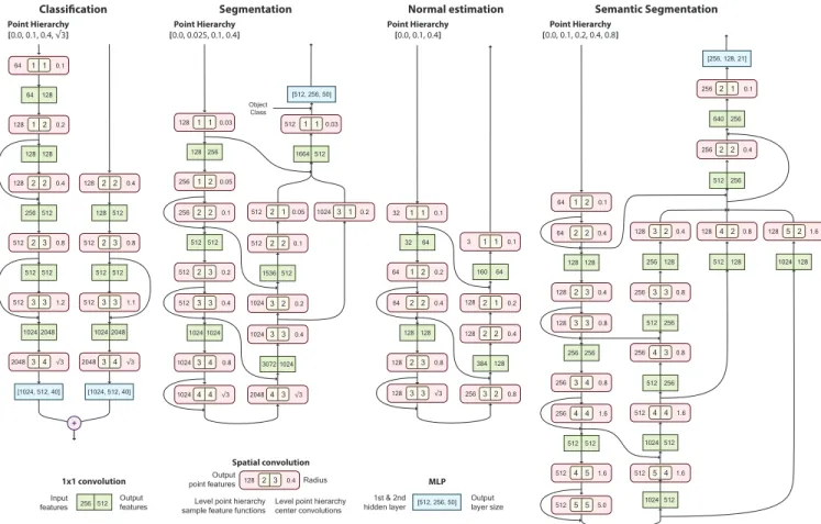
Our classification architecture is composed of several levels (Fig. 11). Each computes a convolution on a point cloud, uses Poisson disk sampling to reduce the number of points, and performs a down-sampling operation to compute the features of the new points.

The convolution of the first level is a multi-feature convolution in order to increase the number of features. However, in deeper levels, we use a single-feature convolution for performance considerations. In order to incorporate combinations of features in such levels, we introduce 1×1 convolutions between the spatial convolutions.

Before each layer, we add a batch normalization layer to improve training, and a ReLU layer to introduce non-linearities. Moreover,

similar to Dense blocks [Huang et al. 2016], we incorporate skip links between the output of the down-sampling layers and the output of the spatial convolution.

The classification network generates a point cloud hierarchy of four levels by iteratively using Poisson Disk sampling on the input point cloud with radius.1,.4, and

√

3 (we use the original point cloud as the first level). The last level (4) is composed of only a single point since the Poisson Disk radius used to compute it was equal to the diagonal of the bounding box.

The final output of the network is a feature vector describing the model which is processed by an MLP with two hidden layers.

In order to increase the robustness of the classification under poor samplings, this architecture was replicated in two different paths, which generate different probability vectors that are added together to create the final class probabilities. However, the second path is composed of only two layers and works directly with the second level of the point cloud hierarchy.

Training.We use cross-entropy loss with an Adam optimizer, a batch size of 32, and an initial learning rate of.005. The learning rate is divided by half after every 20 epoch. To prevent over-fitting we used a drop-out probability of.5 in the final MLPs and a drop-out probability of.2 for the point features before each layer. Moreover, we selected a point from the dataset with a probability of.95, which varied the input points during training. In order to obtain a network robust to models with different samplings, during training, we de-activate one or none of the two paths of the network. The network was trained for 200 epochs.

A.2 Segmentation

This network computes a four-level point hierarchy by iteratively applying our Poisson disk sampling algorithm with radius.025,.1, and.4. It makes use of an encoder-decoder architecture (Fig. 11).

Since the class of the model is assumed as input, as in Point-Net++ [Qi et al. 2017b], we concatenate aone-hotvector containing this information with the output of our network. This information is processed by an MLP composed of two hidden layers with 512 and 256 neurons, and 50 outputs, which generates the parts probabilities.

Training. We trained using a cross-entropy loss with an Adam

optimizer and a batch size of 32. We used an initial learning rate of

.005 which was scaled by.2 every 20 epochs. As in the classification networks, we used a drop out rate of.5 in the final MLP and.2 before each layer. Since in this task we used the complete point set as input, we used a probability of.2 to drop out a point during training. We trained our network for 90 epochs.

A.3 Normal estimation

Our network has an encoder-decoder architecture which generates a point hierarchy of three levels by iteratively applying our Poisson Disk Sampling algorithm with radius.1 and.4.

Training. We used a cosine distance loss using an Adam optimizer and a batch size of 16. Initially, we used a learning rate of.005 which we decreased by half every 20 epochs. We trained our network for 160 epochs.

1 1 0.1 64 128 64 1 2 0.2 128 2 2 0.4 128 256 512 2 3 0.8 512 3 3 1.2 512 1024 2048 3 4 √3 2048 [1024, 512, 40] 128 128 512 512 2 2 0.4 128 128 512 2 3 0.8 512 3 3 1.1 512 1024 2048 3 4 √3 2048 [1024, 512, 40] 512 512 + 1 1 0.03 128 256 128 1 2 0.05 256 2 2 0.1 256 512 512 2 3 0.2 512 3 3 0.4 512 1024 1024 3 4 0.8 1024 4 4 √3 1024 3 2 0.2 3 3 0.4 1024 3072 1024 4 3 √3 2048 1024 1536 512 3 1 0.2 1024 2 1 0.05 512 1664 512 1 1 0.03 512 [512, 256, 50] Object Class 1 1 0.1 32 64 32 1 2 0.2 64 2 2 0.4 64 128 128 2 3 0.8 128 3 3 128 2 1 0.2 2 2 0.4 128 384 128 3 2 256 128 √3 0.8 160 64 1 1 0.1 3

Classification Segmentation Normal estimation

2 3 0.4 128 Radius Output

point features

Spatial convolution

Level point hierarchy center convolutions Level point hierarchy

sample feature functions 256 512

1x1 convolution

Input

features Outputfeatures

MLP

1st & 2nd

hidden layer [512, 256, 50] Outputlayer size

Point Hierarchy

[0.0, 0.1, 0.4,√3] [0.0, 0.025, 0.1, 0.4Point Hierarchy] Point Hierarchy[0.0, 0.1, 0.4]

Semantic Segmentation Point Hierarchy [0.0, 0.1, 0.2, 0.4, 0.8] 2 2 0.4 128 128 64 2 3 0.4 128 3 3 0.8 128 256 256 3 4 0.8 256 4 4 1.6 256 512 512 4 5 1.6 512 5 5 512 4 4 1.6 512 1024 512 5 4 512 [256, 128, 21] 1 2 0.1 64 5.0 1.6 1024 512 512 256 4 3 256 0.8 512 256 3 3 256 0.8 256 128 3 2 128 0.4 512 128 4 2 128 0.8 1024 128 5 2 128 1.6 2 2 0.4 256 512 256 640 256 2 1 0.1 256 2 2 0.1 512

Fig. 11.Network architectures used for the classification, segmentation, normal estimation, and semantic segmentation tasks. The three different building blocks used to generate our networks are described at the bottom of the figure:1×1convolutions, which reduce or increase the number of point features by combining them;Spatial convolutions, which use a level of the point hierarchy as the center of the convolution and another level to sample the feature functions in order to generate a set of new point features; Andmulti-layer perceptrons(MLP), which are composed of three fully-connected layers.

A.4 Semantic segmentation

For the semantic segmentation task on real-world datasets, we use a similar architecture to the one used for the segmentation task. However, since the datasets used in this task are complete rooms of varying size, this network architecture has some differences with the segmentation network (see Fig. 11). The most important difference is that, due to the different sizes of the rooms, we define the radius of our operations in meters, in contrast to the segmentation network in which were defined relative to the bounding box. Moreover, since the point clouds for this task are composed of a higher number of points, the network computes a point hierarchy of 5 levels instead of 4 by applying Poisson Disk sampling with radius .1, .2, .4, and .8 meters. Lastly, in order to reduce the number of operations and the memory consumption, we do not compute a convolution in the first level of the hierarchy. Instead, we use a pooling operation to compute features in the second level based on the input point cloud.

Training.We trained using a cross-entropy loss with an Adam

optimizer. As in the segmentation task, we used an initial learning rate of.005 which was scaled by.2 every 20 epochs. In order to

prevent over-fitting, we used a weight decay factor of 0.0001 and a drop out rate of.5 in the final MLP and.2 before each layer. Moreover, we used a probability of.15 to drop-out a point during training. We trained our network for 100 epochs.

Since the models on the dataset have a varying number of points, in the range of [10 k, 550 k], instead of defining a fixed number of rooms per batch we defined a fixed number of points per batch. Each train step, we select as many rooms as possible until we fill the budget of 600 k points.

Furthermore, the number of points per class is not equally dis-tributed (most of the points belong to the classes_floorand_wall). In order to train a model which is able to classify points for all the classes and not only the most common, we weighted the losses of each individual points based on the class. Moreover, in contrast to previous approaches, we consider all the unannotated points in our input point clouds. However, the loss generated by these points are weighted by 0 and they are not considered during the computation of the performance metric.