University of Mannheim / Department of Economics
Working Paper Series
Capital Adjustment Costs: Implications for Domestic
and Export Sales Dynamics
Yanping Liu
Working Paper 18-04
Capital Adjustment Costs: Implications for Domestic
and Export Sales Dynamics
Yanping Liu
yApril, 2018
Abstract
Theoretical and empirical work on export dynamics has generally assumed constant marginal production cost and therefore ignored domestic product market conditions. However, recent studies have documented a negative contemporaneous correlation be-tween …rms’domestic and export sales growth, suggesting that …rms can be capacity constrained in the short run and face increasing marginal production cost. This paper develops and estimates a dynamic model of export behavior incorporating short-term capacity constraints and endogenous capital investment. Consistent with the empiri-cal evidence, the model features …rms’sales substitutions across markets in the short term, and generates time-varying transition paths of …rm responses through …rms’ capital adjustments over time.
The model is …t to a panel of plant-level data for Colombian manufacturing in-dustries and used to simulate how …rm-responses transition following an exchange-rate devaluation. The results indicate that incorporating capital adjustment costs is quan-titatively important. First, it takes more than …ve years for …rms to fully adjust to a permanent change of the exchange-rate process. Second, the long-run exchange rate elasticity of exports is substantially higher than that in the short run. Firms’expecta-tion on the permanence of the policy changes also matters. The failure to accurately anticipate the duration of the devaluation results in reduction in …rms’pro…ts due to over- or under- investment in capital.
Keywords: International trade; heterogeneous …rms; capacity constraints; capital adjustment costs; …rm dynamics; …rm panel data.
JEL Codes: F12, L11, F14
This version: Apr 2018. First version: Nov 2012. I am grateful to Jonathan Eaton and James Tybout for their guidance, support and encourangement. I have bene…ted greatly from discussions with Russell Cooper, Harald Fadinger, Edward Green, Paul Grieco, Kala Krishna, Volker Nocke, Mark Roberts, Trevor Tombe, Neil Wallace, Daniel Yi Xu and Stephen Yeaple. All remaining errors are mine. Financial support from the European Research Council through grant no. 313623 is gratefully acknowledged.
1
Introduction
How …rms and a country’s overall economy transition following trade liberalization, changes of exchange-rate regime, or vast macro shocks has long been of interest to trade economists, policy-makers and the broader public. While it is a general consensus that trade liberalization and reduction of trade costs increase aggregate trade volume and consumer welfare, the majority of theoretical and empirical work on export responses has focused on the long-run e¤ects of these policies without concerning about the transitional dynamics. Considering that many of …rms’ decisions (capital investment, innovation, export entry, etc) are potentially dynamic1 and a¤ect the return of each other, …rm responses can change over time in their
transition to the long-run steady state. As a result, the overall e¤ects of trade liberalization or market-condition changes will depend on how these …rm responses evolve over time, and how long the transition lasts.
Studies that focus on long-run export responses have generally been conducted under the assumption that …rms face constant marginal production cost. Under this assumption, …rms can expand or contract their production capacity freely without incurring any extra costs beyond marginal production cost. This implies that domestic product market conditions have no e¤ects on …rms’ export decisions2. In particular, when we examine how exports
respond to a trade liberalization, this would imply that …rms can ramp up their production for the export market immediately, and export expansion has no consequences on domestic sales and output price. However, recent studies have documented a negative correlation between exporting …rms’domestic and export sales growth that challenges the assumption of constant marginal production cost. This is shown by Vannoorenberghe (2012), Blum et al (2013) and Ahn and McQuoid (2012), for example. This negative correlation between domestic and export sales growth suggests that …rms can capacity constrained in the short run. However, in these papers capacity is …xed and investment in capital is not allowed.3 As
such they cannot characterize the transition of the economy from the short run to the long run in response to a trade liberalization or changes in the exchange-rate regime.
This paper goes beyond the current literature by developing and estimating a dynamic forward-looking model of …rms’sales dynamics in an open economy with capacity constraints and endogenous investment. It incorporates capital adjustment costs that have been studied
1In the sense that current actions a¤ect future outcomes, and future conditions also a¤ect current decisions
through expectations.
2Domestic factor market conditions, however, would a¤ect …rms’exports through factor prices under the
assumption of constant marginal production cost.
3In Ahn and McQuoid (2012) only …rms that are capacity constrained have …xed capacity. Firms that
typically in the context of a closed economy.4 The model has implications that di¤er from
earlier models that assume constant marginal costs in several respects. First, …rms that are capacity constrained in the short run face a trade-o¤ between domestic and export sales. The increased export sales growth led by positive foreign demand shocks can induce higher output prices for domestic consumers when …rms are capacity constrained. Second, the long-run responses di¤er from the short-long-run responses, as producers can adjust their production capacity through capital investment over time. Finally, producers’ expectations about the duration of policy changes or persistence of external shocks a¤ect their sales responses. The failure to accurately anticipate the persistence of shocks results in reduction in pro…ts due to over- or under- investment in capital.
The paper quanti…es these e¤ects by …tting the model to plant-level panel data from Colombia. The Colombian data is suited for this study as reduced-form empirical evidence suggests that producers cannot easily expand or reduce production capacity in the short run.5 It shows that the inability of …rms to adjust their production capacity a¤ects their
export and domestic sales dynamics. With Colombian plant-level data I also con…rm the substitution behavior between domestic and export sales for exporters, similar to other studies. In addition, I document that expansion in the export market is accompanied by an increase in the plant-level output price index and followed by high investment level.
The model is estimated using a simulated-method-of-moments approach. The calibrated model does a good job in replicating the basic features of the Colombian micro data, including the exporting patterns, correlation between domestic and export sales growth among con-tinuing exporters, correlation between export sales and price, the distribution of investment rates, and the serial correlation of investment rates. The estimates of the model suggest that the idiosyncratic demand shocks dominate productivity shocks in generating …rms’sales vari-ation. The estimated coe¢ cients for capital adjustment costs suggest that both convex and …xed capital adjustment costs exist, and there is substantial price di¤erence in purchasing and selling physical capital.
The calibrated model is then used to conduct policy experiments of changes in the ex-change rate regime. The experiment simulates the transitional dynamics of domestic and export sales, price and capital investment from the short run to the long run in response to the policy changes. The results show that incorporating capital adjustment costs is empiri-cally important, and …rms’expectation on the duration of the policy changes matters. First, it takes more than …ve years for …rms to fully adjust to a permanent change of the exchange-rate process that depreciates the steady state value of the peso by 20%. The long-run and
4Papers include Caballero and Engel (1999) and Cooper and Haltiwanger (2006), etc. 5This paper uses …rm and plant interchangeably.
short-run export responses also di¤er: the long-run exchange rate elasticity of exports is 30% higher than that in the short run. Finally, …rms’ anticipation and expecation on the per-manence of the policy changes also matters. (1) When …rms correctly perceive a temporary currency devaluation, …rms substitute their domestic sales towards the export market. There are no responses in capital adjustments. (2) When the devaluation is temporary but …rms incorrectly perceive it to be permanent, …rms over-invest in capital and su¤er reductions in pro…t due to increased capital adjustment costs induced by over-investing and downsizing the capital afterward. (3) When the devaluation is permanent but …rms incorrectly perceive it to be temporary, …rms under-invest in their capacity and the substitution of domestic sales for export sales is prolonged. Firms incur reductions in pro…t because of the increased marginal cost caused by insu¢ cient capital investment. Domestic consumers also incur wel-fare losses because of the prolonged periods of high price. (4) When …rms correctly perceive permanent currency devaluation, the substitution away from domestic sales for exports is temporary. Firms bring back their domestic sales after they invest in physical capital.
Relation to the Literature This paper is most closely related to contemporaneous work by Rho and Rodrigue (2015, forthcoming). Rho and Rodrigue (2015) focus on capital investment and growth patterns of new exporters compared with non-exporters, featuring increasing marginal production cost (MC) and capital adjustment costs similar to our setting. They show estimates of sunk export entry cost and per-period export …xed cost are over-estimated for models assuming constant MC and no capital adjustment costs by applying their model to two Thailand manufacturing industries. This paper di¤er from Rho and Rodrigue in several dimensions. First, this paper utilizes output price data at the plant-level to separate plants’ cost and demand shocks, while Rho and Rodrigue (2015) back out a plant’s foreign demand from observed export intensity, assuming domestic demand is the same across plants. This is important as it has di¤erent implications on the correlation between sales growth and a¤ects the productivity estimates. Secondly, this paper focuses on both new and incumbent exporters, while Rho and Rodrigue (2015) largely focus on new exporters.
The paper relates to some recent works that study capacity constraints and export be-havior. Vannoorenberghe (2012) establishes reduce-form evidence of negative correlation between output variation on the domestic and export market at the …rm level, suggest-ing short-run convex production cost as an explanation. Blum et at (2013) and Ahn and McQuoid (2012) also provide empirical evidence that supports the view of exporting …rms being capacity constrained. Ahn and McQuoid (2012) use …rm-level data from the Indone-sian wood industry and established a negative correlation between plants’ domestic and export sales growth. The authors …nd stronger negative correlation between domestic and
export sales for plants that are either …nancially or physically constrained than those who are not constrained through reduce-form analysis. While Ahn and McQuoid (2012) treat producers’capacity constraints as exogenous and …xed, this paper focuses on the dynamic adjustments of physical capital that a¤ect the extent to which producers being constrained. As a result of relaxing producers’ capacity constraints though capital investment, the dy-namic correlation between producers’domestic and export sales growth can be di¤erent from their contemporaneous correlation6.
Blum et al (2013) also document the trade-o¤ between selling domestically and abroad based on Chilean …rm-level data. They …nd that a large fraction of …rms enter and exit the same export destination multiple times, and sell the same products to the same importers upon re-entry. They attribute this behavior to …rms facing limited production capacity. The paper classify exporters as either "occasional" or "perennial" exporters depending on the number of exporting spells and the length of the exporting spell. Their reduce-form analysis …nd that occasional exporters reduce their domestic sales when entering into exporting, but it is not the case for perennial exporters. In addition, there is a negative correlation between changes in domestic and foreign sales for continuing exporters. Again in Blum et al (2013) producers’production capacity is …xed and can not be adjusted through capital investment after a producer starts exporting. Instead, in this paper we focus not only on the trade-o¤ between selling in the domestic and foreign market but also the dynamic adjustment of production capacity through capital investment. Similarly, Almunia et al (2018) document a larger increase of export ‡ow for …rms with a larger reduction in domestic demand using Spanish data during the Great Recession. Soderbery (2014) also presents a model where …rms have heterogeneous and …xed capacity, and show trade liberalization could negatively impact welfare through …rms raising output price.
Another closely related paper is Artuc et al (2013). While the patterns Ahn and McQuoid (2012) and Blum et al (2013) focus on are mostly static, Artuc et al (2013) look at the dynamic adjustments of capital investment and labor in response to exogenous trade shocks based on Argentine data under capital adjustment costs and workers’mobility costs. What it di¤ers from this paper is that Artuc et al (2013) do not look at …rms’exporting decisions and mainly focus on the factor market adjustments. In this paper we are also interested in the implications of factor adjustments on the interrelation between producers’domestic and export sales dynamics.
This paper is also related to a broader literature that study export dynamics, including
6Exceptionally, Berman et al (2015) shows positive correlation between variation in foreign and domestic
sales based on French …rm-level data. They point to a relaxation of short-run liquidity constraints as the reason for such positive correlation.
Alessandria and Choi (2014), Arkolakis (forthcoming), Eaton et al (2014), Arkolakis, Eaton and Kortum (2012), Das et al (2007) and Ruhl and Willis (2007, 2015). This paper di¤ers from Arkolakis, Eaton and Kortum (2012), Eaton et al (2010), Arkolakis (2010, forthcoming) and Ruhl and Willis (2015) in that it focuses on frictions in the factor market. Alessandria and Choi (2014) develop a general equilibrium model featuring sunk export costs and capital accumulation, emphasizing the contribution of extensive margin to aggregate exports. Ruhl and Willis (2007) look at labor market frictions, but their focus is on new exporter growth and they ignore the domestic product market. This paper di¤ers from theirs in two ways. 1) It introduces idiosyncratic demand shocks besides productivity shocks; 2) This paper also looks at …rms’sales substitution patterns between the domestic and export market, and the correlation between price and sales growth, which are not the focus of Ruhl and Willis (2007). The paper is also related to Riano (2011) which studies exports and capital investment. But the focus of Riano (2011) is on …rm-level sales volatility.
Another strand of literature that this paper relates to includes research that studies cap-ital adjustment costs and their implications on the aggregate economy. Caballero and Engel (1999), as well as Cooper and Haltiwanger (2006), have argued that non-convex adjustment costs lead to lumpy investment decisions and aggregate nonlinearity. Contreras (2008) looks at the joint adjustment and interrelation of capital and labor using Colombian plant-level data from year 1982 to 1998. Contreras (2008) …nds empirical support for congestion e¤ects which means adjusting capital and labor at the same time is more costly than adjusting them separately. While these studies focus on a closed economy, this paper explores the im-plication of capital adjustment costs on domestic and export sales dynamics in the context of an open economy.
The remainder of the paper proceeds as follows: Section 2 presents the structural model. Section 3 provides descriptive analysis of the Colombian plant-level data used in this paper. Section 4 conducts the quantitative analysis that …ts the model to the data. Section 5 concludes the paper.
2
Model
The model features a small open economy where exchange rate and foreign market-size are independent of domestic market conditions. It builds on the existing models of …rm hetero-geneity and exporting. Firms are heterogeneous in terms of both their underlying e¢ ciency and market-speci…c demand shocks. Exporting to the foreign market entails …xed costs that are paid every period, as in Melitz (2003). Therefore only a fraction of domestic …rms ex-port. Firms switch into or out of exporting as they experience demand and productivity
shocks, as in Das et al (2007). What this paper adds to these models is a characterization of the relationship between …rms’export behavior and their capital formation. Firms’capital assets are …xed in the short run and face increasing marginal production cost, thus there is a trade-o¤ between the domestic and export sales for exporters. Firms make investment choices given their perception about future market conditions.
The supply side of the model features heterogeneous …rms located in the home country with di¤erent productivity levels. Each …rm produces a single variety using standard Cobb-Douglas technology. The factors of production are labor and physical capital. Labor is variable input that can be freely adjusted at any time, while the amount of physical capital is …xed in the short run. The …rms’inability to adjust physical capital in the short run leads to increasing marginal production cost. Over time physical capital can be adjusted through investment but subject to capital adjustment costs.
On the demand side, there is heterogeneous demand for each …rm’s variety in both the domestic and foreign market. I do not endogenously model demand growth through …rms’ searching and accumulating customers, or learning about the popularity of their products. This is mainly because I do not observe the necessary demand-side data to do so.
2.1
Demand
The domestic and foreign countries d and f have a continuum of consumers. Consumers in both countries have identical CES preferences with the same elasticity of substitution . There is a mass one of varieties available, each produced by a single …rm from the domestic country. Consumers in countryk2 fd; fghave incomeEk
t. A representative consumer from
countryk maximizes its utility
Utk =
Z
ztk(j)1qtk(j) 1dj
1
, k 2 fd; fg
subject to the budget constraint
Z
pkt(j)qtk(j)dj =Etk, k 2 fd; fg
wherezk
t(j)is the product appeal of productj at countryk, or the weight that consumer in
countryk place on productj,qk
k, andpk
t(j) is varietyj’s price at countryk7. The demand for product j at country k is
qtk(j) =ztk(j)p k t(j) (Pk t)1 Etk, k 2 fd; fg wherePtk= (R ztk(j)pkt(j)1 dj)11 . DenoteDk jt =ztk(j) Ek t (Pk
t)1 ;The total demand for variety
j from country k is
qkjt = (pkjt) Djtk, k2 fd; fg (1)
Note that both foreign pricepfjt and incomeEtf are based on foreign currency here. They are going to be switched to domestic currency when calculate the …rm’s total revenue.
2.2
Production
On the supply side, each …rm produces a single variety and …rms compete monopolistically. Firms are heterogeneous in their productivity levels Ajt. They employ a Cobb-Douglas
production technology with two factors: labor and physical capital. Labor is a variable input so it can be freely adjusted in each period. However, the amount of physical capital in a given period is …xed. The production function for …rmj at time t is
qjt =AjtKjtkL
l
jt
Given …rmj’s capital levelKjt, wagew, its marginal production cost as a function of its
output qjt is: M Cjt = w l q 1 l 1 jt A 1 l jt K k l jt (2)
The total variable production cost is
T V Cjt =wq 1 l jt A 1 l jt K k l jt (3)
Marginal cost M Cjt is therefore an increasing function of its total outputqjt as long as the
labor share l is less than 1. In addition, the higher the …rm’s productivity Ajt and capital
level Kjt, the lower its marginal production cost is.
2.3
Static problem
In the beginning of each period, a …rm observes its productivity and demand shock in both the domestic and foreign market. Given its capital level, the …rm chooses its output, whether
to export or not, and if so, the allocation of its output in the domestic and foreign market. Exporting entails a per-period …xed cost f, therefore only …rms with productivity or foreign demand above a certain level exports. Denote jt as the share of its total production that is sold abroad, so qfjt = jtqjt. I solve the problem in two steps: (1) Given a …rm’s
output qjt, a …rm decides its export share jt if it exports. (2) Given the optimal export
share if it exports, a …rm decides the optimal outputqjt and whether to export or not. Based
on the demand function (1), the …rm’s total revenue in domestic currency if it exports is
S(Ajt; Kjt; Djtd; D f jt; et) = max jt2[0;1] pdjt(1 jt)qjt+etp f jt jtqjt = max jt2[0;1] h (1 jt) 1(Djtd)1 +et( jt) 1 (Dfjt)1i(qjt) 1
Hereet denotes the exchange rate: 1 unit of foreign currency worth et domestic currency at
time t.
We can solve for the optimal export share jt by maximization of the above equation. The optimal jt for an exporting …rm is
jt = 1 + Dd jt Djtfet ! 1 qfjt qd jt = D f jtet Dd jt pfjt pd jt = (q f jt Dfjt) 1 (q d jt Dd jt ) 1 = 1 et
pfjt is the price a …rm charges abroad in foreign currency, therefore we can denote a …rm-level price in domestic currency:
pjt =etp f jt =p
d
jt (4)
This property relies on the assumption that the demand elasticity is the same for both domestic and foreign consumers. Under this assumption …rms do not price discriminate across markets. The optimal export share jt only depends on the demand shocks and the exchange rate, but not on the total output level. So essentially the …rm faces a world-wide demand and charges the same price. Denote xjt 2 f0;1g as an indicator of …rm
Dd jt+ (D f jtet) 1(xjt = 1), equivalently, Djt = ( (Ddjt+Djtfet); if export: xjt = 1 Djtd; if not export: xjt = 0
The optimal export share implies the revenue for the …rm becomes
Sxjt(Ajt; Kjt; Ddjt; D f jt; et) = (Djt) 1 (qjt) 1
Given the revenue a …rm can potentially get by selling to both markets at any given output level, the …rm decides whether to export or not and the amount to produce by solving the problem below:
max qjt;xjt2f0;1g Sxjt(A jt; Kjt; Djtd; D f jt; et) T V C(Ajt; Kjt; qjt) f 1(xjt = 1)
The optimization problem implies the optimal quantity to produce, revenue and total variable cost to be: qjt = 1 l w(AjtK k jt ) 1 l(Djt) 1 1 1 l 1 S(Ajt; Kjt; Ddjt; D f jt; et) = ( 1 l w) c3(D jt)c2 (AjtKjtk) 1 l c3 T V C(Ajt; Kjt; Ddjt; D f jt; et) = w( 1 l w) 1+c3(D jt)c2 (AjtKjtk) 1 l c3 where c1 = 1 1 l 1, c2 = 1 1 l 1 1 l 1,c3 = 1 1 1 l
1.The superscript xjt which indicates
the export status is omitted, as it is captured in the aggregate demand shock: Djt =Djtd +
(Djtfet) 1(xjt = 1):Note that the productivity and demand shocks, capital enter the revenue
and total variable cost function in the same way, thus total variable cost is a fraction of a …rm’s total revenue: T V C(Ajt; Kjt; Djtd; D f jt; et) S(Ajt; Kjt; Ddjt; D f jt; et) = 1 l (5)
Therefore a …rm’s per-period pro…t is:
xjt(A jt; Kjt; Ddjt; D f jt; et) = (1 1 l)S(Ajt; Kjt; Ddjt; D f jt; et) f 1(xjt = 1)
selling in the domestic market alone: xjt=1(A jt; Kjt; Ddjt; D f jt; et) xjt=0(Ajt; Kjt; Ddjt; D f jt; et)>0 =) xjt = 1
It’s worth noting that export participation is a static choice since exporting involves only per-period …xed cost but no sunk cost by assumption.
2.4
Dynamic Problem
The problem is dynamic because a …rm’s current investment decision a¤ects its future capital stock and production capacity. The state variables include capital stock Kjt; productivity
Ajt, …rm speci…c demand shocks Ddjt; D f
jt, and the exchange rate et. Capital stock Kjt is
the only endogenous state variable and the rest are exogenous. An incumbent producer in the domestic market chooses the capital investment to maximize the value of continuing operating in the market:
V(Ajt; Kjt; Djtd; D f jt; et) = (6) max Ijt (Ajt; Kjt; Ddjt; D f jt; et) (Ijt; Kjt) + 1 1 +rEV(Ajt+1;(1 )Kjt+Ijt; D d jt+1; D f jt+1; et+1jAjt; Djtd; D f jt; et)
where Kjt+1 = (1 )Kjt+Ijt. (Ijt; Kjt) is the associated capital adjustment costs. The
functional form for (Ijt; Kjt) is provided in section 2.6. 1+1r is the discount rate for next
period’s pro…ts. The value function is comprised of the current pro…t and discounted future pro…ts net of the capital adjustment costs associated with the investment.
Note that export status is not a state variable here because there is no sunk entry cost for new exporters. For simpli…cation the entry and exit into production are not modeled.
2.5
Functional Forms
To solve the model numerically, the log of productivity Ajt; idiosyncratic demand shocks
Ddjt; Djtf and real exchange-rate are assumed to follow independent …rst-order autoregressive processes:
lnAjt = ma+ alnAjt 1+"ajt lnDjtd = md+ dlnDdjt+"djt lnDjtf = mf + flnD f jt +" f jt lnet = me+ elnet 1+"et where "ajt i:i:d:N(0; 2a), ("djt; " f jt) i:i:d:N(0; 2 d; df d f; df d f, 2f ); "et
i:i:d:N(0; 2e): df allows the innovations to the domestic and foreign demand shocks to
be correlated. Given these functional forms, the expected future valueEV(jAjt; Djtd; D f jt; et)
in the value function can be parameterized.
2.6
Capital Adjustment Costs
The evolution of …rmj’s capital stock follows
Kjt+1 = (1 )Kjt+Ijt
where is the depreciation rate and Ijt is the capital investment. The investment rate,
ijt = KIjt
jt can be either positive or negative. There is one-period time-to-build, so investment
made at period t becomes e¤ective at period t+ 1.
In addition to the time to build assumption, adjusting the capital stock is costly. The capital adjustment cost function is speci…ed as:
(Ijt; Kjt) = 1 2 Ijt Kjt 2 Kjt+ 21(j Ijt Kjtj >0)Kjt+Ijt1(Ijt >0) 3Ijt1(Ijt <0) (7)
The adjustment costs include a quadratic cost 1
2
Ijt
Kjt
2
Kjt that is usually assumed in
traditional investment models, a …xed cost of adjustment 2, and transaction costs 3 that
captures a gap between the buying and selling price of capital. This speci…cation is close to that of Cooper and Haltiwanger (2006).8 The convex costs dampens the investment responses to shocks and lead to partial adjustment of investment. The …xed cost of adjustment 2Kjt
is independent of the level of investment. It is proportional to the level of capital to eliminate any size e¤ect. Compared with partial adjustment implied by the convex costs, the …xed adjustment costs imply frequent investment inactivity and investment spikes. The price gap
8The only di¤erence is that Cooper and Haltiwanger (2006) incoporats an additional type of non-convex
adjustment cost that represents a loss of a fraction of the output during the adjustment period. Since their implications are similar to the …xed adjustment costs, I only keep the …xed adjustment costs for simpli…cation.
between purchasing and selling capital would also dampen …rms’ investment responses to positive productivity or demand shocks, as selling the capital in the future would incur a loss. In addition, the price gap imply that …rms will hold on to capital in response to a negative shock.
3
Data
The data used in this paper is a plant-level dataset collected by Departamento Administrativo Nacional de Estadística (DANE). It covers all manufacturing plants with more than ten employees from year 1981 to 1998. However information on exporting is not included for years after 1991, and information on output price is not included for year 19819. For this
reason I only use the data from 1982 to 1991. As the focus of the paper is the sales and capital adjustment of an existing plants, I keep a balanced sample and drop the plants that enter or exit the panel in the middle of the sample period. I keep 19 major exporting industries in the Colombian manufacturing sector, as in Roberts and Tybout (1997)10. This leaves a total number of 2235 plants for 11 years.
The data set contains plant-level information on each plant including its age, industry classi…cation (four digits SIC), capital stocks, investment ‡ows, employment, expenditure on labor and capital, value of output sold in the domestic market and value of output exported. Each plant’s export sales are aggregated across all export markets and we do not observe their destinations and export sales for individual destination. The data also includes a plant-level price index for output and materials. However we do not observe the domestic and foreign output price separately for exporting plants11
Plant-level price indices: The plant-level output price indices are constructed by Eslava et al. (2004). Output price indices are constructed using Tornqvist indices. For a plant that produces multiple products, the output price indices are constructed based the weighted average of the growth in prices for all individual products produced by that plant.
9The data set used in Eslava et al. (2004) covers the years from 1982 to 1998. It includes price information
but not information on export sales. The data set used in Roberts and Tybout (1997) covers the years from 1981 to 1991 which does not have price information. Therefore we merged the two data sets based on plant’s industry classi…cation, employment level, energy usage. About 90% of the observations between 1982 and 1991 are matched after the merging.
10The 19 industries are: food processing, textiles, clothing, leather products, paper, printing, chemicals,
plastic, glass, nonmetal products, iron and steel, metal products, machinery, transportation equipment, and miscellaneous manufacturing.
11In the CES model under the assumption that demand elasticities are the same at home and abroad, the
foreign price and domestic price collapse into one price, as shown in equation (4) in the model section. This price index provides useful information to separately identify the productivity and demand processes. Also the price responses to shocks reveal how easily …rms can adjust their production capacity.
For plant j at time t producing producth = 1;2; :::; H, the weighted average of the growth of price is given by:
Pjt = H X h=1 shjt ln(Phjt) where ln(Phjt) = lnPhjt lnPhjt 1 and shjt= shjt+shjt 1 2
where Phjt and Phjt 1 are the prices charges for product h by plant j at time t and t 1;
shjt and shjt 1 are the share of producth in plant j’s total production for years t and t 1.
The indices for the level of output prices for each plantj are constructed using the weighted average of the growth of the prices with year 1982 being the base year:
lnPjt = lnPjt 1+ Pjt
for t >1982, where Pj1982 = 100. The price levels are obtained by applying an exponential
function to the natural log of prices, Pjt = explnPjt: Material price indices are similarly
constructed based on price and value share of each material used in the production process.
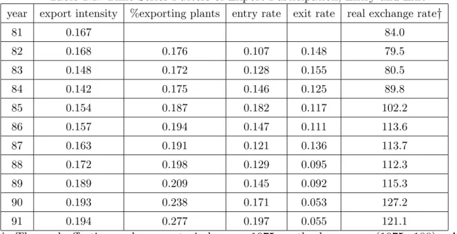
Export Participation, Entry and Exit: The time-series patterns of export partici-pation, export entry and exit among existing domestic producers over the sample period are summarized in Table 1.1. These patterns follow closely the movement in the real exchange rate. From the middle of 1970s until 1982 the Colombian peso appreciated steadily, and then depreciated steadily until 1986. After being stabilized from 1986 to 1989, it appreciate slightly from 1989 to 199012. The fraction of plants that export among existing domestic producers for the major exporting industries fell in the beginning of the 1980s, then started to increase since 1984. Export participation increased greatly in 1990 and 1991 which are 23.8% and 27.7% respectively. The fourth and …fth row of Table 1.1 presents the entry rate (export at t but not t-1) and exit rate (export at t-1 but not t) of exporting among incumbent domestic producers. The export entry rate at year t is the percentage of plants that export at t but not yet t-1, as a fraction of exporting plants at year t. The exit rate is the percentage of plants that export at year t-1 but stop exporting at year t. The enter rate varies from 10.7% to 19.7% during the sampling years. In general for years the exchange-rate
12Roberts and Tybout (1997) pointed out the appreciation of the Colombian peso from mid-1970’s to 1982
was a response to illegal exports, foreign-capital in‡ows and a boom in the co¤ee market. The appreciation of the currency in the 1980’s was partly a result of the central-bank currency-market interventions to ease competitive pressure on tradable-goods producers.
is favorable for Colombian exporters, the export enter rate tends to be high and the exit rate tends to be low.
3.1
Patterns of Capital and Labor adjustments
This section presents some basic patterns on how plants dynamically adjust their use of capital and labor which re‡ect the nature of the underlying adjustment costs. As established in the literature (e.g., Cooper and Haltiwanger (2006)), I …nd that investment adjustment is lumpy with frequent investment spikes and inaction, and its distribution is asymmetric with few observations of negative investment. Compared with capital adjustment, the adjustment of labor is smoother with more frequent medium-size adjustments. The distribution of labor adjustment is symmetric. Compared with physical capital, labor adjustment is more responsive to shocks. The combined facts suggest that labor is more ‡exible to be adjusted than physical capital.
The analysis conducted here is similar to Contreras (2008). While Contreras (2008) focuses on factors including capital, labor, materials and energy, here I look at capital and labor inputs only. In addition, the analysis in Contreras (2008) regarding the interrelations between the adjustments for di¤erent inputs is conditional on estimates of demand and productivity shocks from Eslava et al. (2004), while here I only look at the unconditional relationships between the factor adjustments.
Distributions of Capital and Labor Adjustments: The distribution for capital and labor growth is shown in Table 1.2. We can see that capital adjustment is lumpy with frequent investment inactions and spikes. This can be seen from the high fraction of observations with investment rate above 20%, and the high fraction of observations with zero or near-zero capital investment. This suggests the existence of …xed cost in adjusting capital. Under …xed adjustment cost, plants would reduce the frequency of adjustment. That implies that they would over-shoot when they do adjust, or simply let the capital depreciate. Compared with the lumpiness of capital adjustment, labor adjustment is relatively smooth, as the proportion of large adjustments is small relative to the proportion of medium-size adjustments.
In addition to the lumpiness of capital adjustment, the capital investment rate distri-bution also exhibits asymmetry with a very small proportion of negative investment. The asymmetry re‡ects the irreversibility of capital investment, which can be a result of a low selling price of capital compared with the purchasing price due to a lack of a secondary market. On the other hand, the distribution for labor growth rate is fairy symmetric.
Contemporaneous and Serial Correlations: To illustrate how capital and labor adjustments and sales growth are interrelated, Table 1.3 presents the contemporaneous relations between capital, labor and total sales growth rate. There is a high positive cor-relation between labor growth and total sales growth Corr( Ljt
Ljt ;
Stotal jt
Stotal jt
), which can be due to a high labor adjustment in response to a positive pro…t shock, as a pro…t shock would also increase sales. The correlation between sales growth and subsequent capital growth
Corr( Kjt Kjt ; Stotal jt Stotal jt
) is also positive, but smaller than that between labor and total sales growth. It indirectly suggest labor adjustment is more ‡exible than capital adjustment. The correlation between capital and labor adjustment is slightly positive. This positive correla-tion can be due to both factors responding to pro…t shock, but can also be dependent on the adjustment cost that makes …rms to adjust both factors together.
Table 1.4 shows the probability of having an investment spike conditional on having an labor growth spike, and vice versa. The results come from a logit estimation. We can see that having a labor adjustment spike increases the probability of having an investment spike, and vice versa. Again the adjustment in both capital and labor together can be due to both factors responding to positive shocks.
The serial correlation of labor, capital and total sales growth are shown in Table 1.5. The serial correlation for total sales growth and labor growth are close and both are slightly negative. If we believe the pro…t shock follows an autoregression process, then the serial correlation of sales growth would be negative. We would also see negative correlation for the factor growth if the factors adjust perfectly in response to the shocks. The serial correlation for capital growth is slightly positive. It can be a mixed e¤ect of both convex and …xed costs of adjusting capital. The convex cost leads to a positive serial correlation of capital growth as plants’tend to make partial adjustment in capital under convex costs. Table 1.6 looks at the dynamic relationship between capital and labor growth. Having a high labor growth in the previous period have a positive e¤ect on the subsequent-year capital growth, and having a high capital growth also signals a higher labor growth later.
3.2
Capacity Constraints, Domestic and Export Sales Dynamics
After establishing the factor adjustment and exporting patterns, we now turn to explore the interactions between factor adjustments and producers’export and domestic sales dynamics. Below I present key features of the data that characterize the interactions between domestic and export sales, plant-level price and physical capital at the micro-level. First, there is a robust negative correlation between exporting producers’domestic and export sales growth. In particular, the expected growth rate for domestic sales is negative for producers that
have experienced a high export sales growth. In addition, the sales substitution13 and the
expansion in the export market is accompanied by an increase in the plant-level output price index. Third, the sales substitution and export expansion is followed by a high level of capital investment. Finally, compared with a strong negative contemporaneous relationship between domestic and export sales growth, the dynamic relationship between domestic and export sales growth is slightly positive but not strong. I discuss each of these features in detail below.
Contemporaneous Correlation between Domestic and Export Sales Growth:
The key feature that suggests plants cannot easily adjust their production capacity in the short run is the substitution between exporters’domestic and export sales. Substitution be-tween domestic and foreign sales could happen when plants receive a more favorable demand shock in one market relative to the other and it is costly for plants to adjust their production capacity. The sales substitution across markets is shown by a negative correlation between …rms’domestic and export sales growth rate14. It can be seen from a simple OLS regression
of an exporter’s domestic sales growth S
d jt
St jt
on its export sales growth S
f jt St jt : Sdjt Stotal jt = 0+ 1 S f jt Stotal jt +"jt
The coe¢ cient (standard error in parentheses) 1 = 0:228(:025 ) is negative and statisti-cally signi…cant. Here export and domestic sales growth are de…ned as15:
Sjtf Stotal jt = S f jt S f jt 1 1 2(S total jt +Sjttotal1) Sd jt Stotal jt = S d jt Sjtd 1 1 2(S total jt +Sjttotal1)
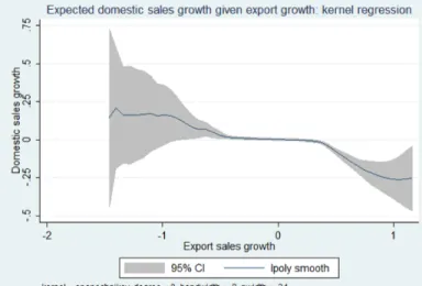
Figure 1 plots the results from a kernel regression of domestic sales growth on export sales growth. It depicts the mean domestic sales growth conditional on plants’export sales growth. We can see that without imposing a linear relationship between the two variable, the negative
13A sales substitution is loosely de…ned as an incidence when an exporter increases its sales in one market
and decrease sales in the other.
14The focus here is the relationship between domestic and export sales growth, rather than that between
domestic and export sales in scale. The latter is positive as usually more productive …rms sell more both at home and abroad.
15Sf
jt; Sjtd;andSjtt indicate a plant’s export, domestic and total sales separately. The export sales growth
rate for plantj at year tis calculated as the di¤erence of export sales between yeart andt 1 divided by the mean total sales between yeartandt 1, and similarly for domestic sales growth. The growth rates for domestic and export sales are both weighted by the total sales so they are comparable.
relationship between domestic and export sales growth is still robust. It shows that plants that expand signi…cantly in the export market reduce their domestic sales even though their total sales grow, suggesting those plants can be capacity constrained. In contrast, plants that contract their export sales increase their domestic sales even though their total sales decline. The conjecture is that these plants su¤er a bad demand shock in the foreign market. They temporarily reallocate their output away from the foreign market towards the domestic market because it’s costly to reduce the production capacity.
Correlation between Price and Sales Growth: In additional to the sales substi-tution patterns, changes in the plant-level output price provide further support for those plants either being capacity constrained or having excess capacity. The idea is that if plants are capacity constrained when the level of their output fails to keep up pace with demand, output-price should go up. To the contrary, if plants have excess capacity and output is beyond the market demand, then price should fall. An OLS regression of the price growth rate on export sales growth rate shows a positive correlation:
pjt pjt = 0 + 1 Sfjt Stotal jt +"jt
The coe¢ cient (standard error in parentheses) 1 = 0:121(0:029 )is positive and statistically
signi…cant. Price growth pjt
pjt is de…ned as pjt pjt = pjt pjt 1 1 2(pjt+pjt 1)
. The way how this plant-level output price indice pjt is constructed is described in data section above.
Figure 2 plots the results from a kernel regression of output price growth on export sales growth. It depicts the expected output-price growth conditional on plants’ export sales growth. Again the positive relationship is robust and does not depend on the linearity assumption. An high export sales growth is accompanied by an increase in the output-price. For the plants that expand in the export market and decrease their domestic sales which suggest them being capacity constrained, we also see an increase in the plant-level price. On the contrary, we observe a price decrease for the plants that contract their export sales and increase domestic sales.
The availability of plant-level price indices is potentially useful in separately identify-ing the e¤ects of heterogeneous productivity and demand shocks. Without establish-level price information much of the existing literature measures output as revenue de‡ated by a common industry-level price index. Therefore their productivity measures embody both the idiosyncratic demand shifts and e¢ ciency. The ability to measure plant-level prices can help with correcting the measurement errors. Separating e¢ ciency and demand shocks is particularly important for the question of interest in this paper as the source of shocks
af-fects the interrelation of domestic and export sales under factor adjustment costs. While the e¢ ciency shocks lead to a positive correlation of exporting producers’domestic and export sales growth, demand shocks can induce a negative correlation of the two variables under physical capacity constraints.
Table 1.7 explores further whether having a sales substitution have an additional e¤ect on the price growth. The dummy for a sales substitution equals to one if an exporting plant’s sales growth is positive for one market and negative for the other market. The idea is to see if having a sales substitution to some extent indicates a plant being capacity constrained and puts an upward pressure on output prices. The second column reports the results of a regression of price growth on export sales growth and also the sales substitution dummy. Conditional on the export sales growth, the e¤ect of having a sales substitution is close to zero and not statistically signi…cant. The third column looked at the e¤ects of total sales growth instead of export sales growth. The e¤ect of total sales growth on price growth is similar to that of export sales growth, and again the e¤ect of having a sales substitution is not signi…cant.
The coe¢ cient for the sales substitution dummy being insigni…cant, however, is not in contradiction with those plants with sales substitution being capacity constrained. It only states that having sales in both markets moving in opposite direction does not a higher price e¤ect than having domestic and export sales moving in the same direction. This largely depend on the source of the shocks. If plants have sales in both markets grow in respond to positive demand shocks in both markets, we do not expect the price e¤ect to be lower compared with the case where plants have sale grow in one market and fall in the other market.
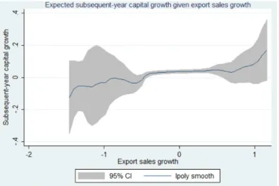
Sales Growth and Subsequent Capital Growth16: Plants’adjustment in capital in response to export sales growth is summarized in Figure 3. It plots the results from a kernel regression of subsequent-period capital growth on export sales growth. There is a robust positive relationship between the mean capital growth and export sales growth for exporting plants. The capital growth rate is de…ned as GKi;t =
Ki;t Ki;t 1
0:5 (Ki;t 1+Ki;t). The plants that are
suggested to be capacity constrained have high capital growth rateGKi;t in the subsequent
period. On the contrary, those plants that are believed to have excess capacity, have near zero or negative capital growth rate. The fact that we do not see much negative capital growth rate partly re‡ects the irreversibility of capital, that is, there is a price gap between
16Some studies …nd investment in advance of exporting, e.g., Bustos (2010). For new exporters that survive
their early exporting years, I also …nd that their is an increase in investment one year prior to and the year of their export entry. But the investment is more substantial during the years after their entry into the export market.
buying and selling the capital. Therefore …rms may choose to hold on to instead of selling the capital in response to negative shocks.
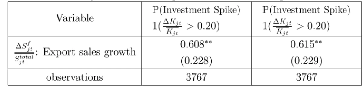
Table 1.8 looks at the probability of having a spike in capital growth conditional on export sales growth. It shows the result of estimating a logit model, where the dependent variable is a dummy for having an investment spike de…ned as 1( Kjt
Kjt >0:20), and the independent
variable is export sales growth. The logit estimation is to show the comovement between growth in export sales and capital in the subsequent period, which depends on both the exogenous shocks and also the underlying adjustment costs. We can see that the probability of having an investment spike increases when there is a high growth in the plant’s export sales.
Dynamic relationship between Domestic and Export Sales Growth: Figure 4 depicts the mean domestic sales growth in the subsequent year S
d jt+1
Stotal jt
conditional on the current export sales growth S
f jt
Stotal jt
. The relationship is slightly positive but not very strong, comparing with a robust negative contemporaneous relationship between domestic and export sales growth shown in Figure 1. In particular, those plants that substitute their domestic sales towards the foreign market in the previous year, have a faster growth rate of domestic sales than that of an average plant in the following year. This suggests these previously capacity-constrained plants bring up their output by investing in capital.
In summary, the empirical evidence above supports the argument that the inability for plants to freely adjust their production capacity in the short run induces substitution be-havior between plants’domestic and export sales, as well as the corresponding output price changes. It also shows that plants adjust their production capacity through capital invest-ment over time, which leads to a di¤erent dynamic correlation between domestic and export sales growth compared with their contemporaneous correlation.
4
Quantitative Analysis
4.1
Fitting the Model to Data
In …tting the model to data, I calibrate the parameters of the model to replicate features of Colombian micro data. First, The real-exchange rate process is estimated using the real exchange-rate series. Second, the production function parameters are calibrated based on the wage share of …rms. I also …x some parameters at values reported by previous studies. Finally, the remaining parameters are estimated to match a set of moments based on …rm-level behavior.
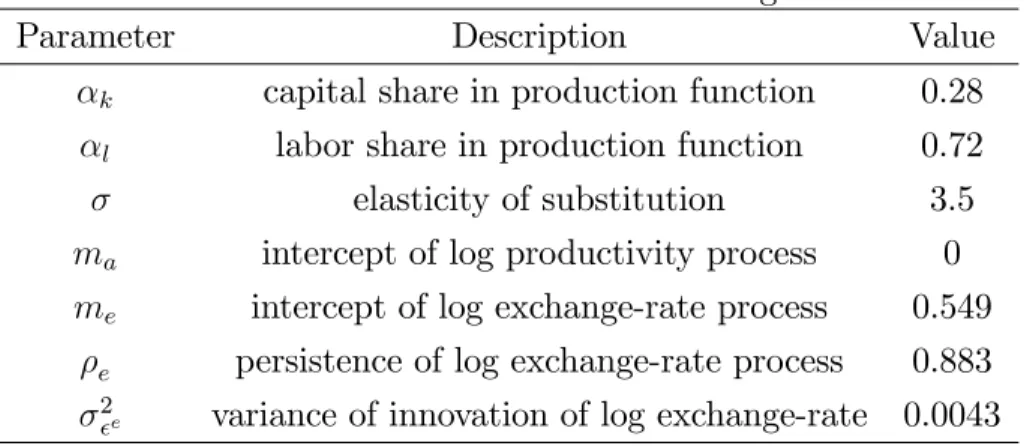
4.1.1 Pre-determined parameters
Table 1.9 summarizes the parameters that are set or estimated without solving the model. Some standard parameters are …xed at values reported by previous studies. First, the real borrowing rater is set to be 0.15 (Bond et al, forthcoming). The depreciation rate of capital is set to be 7%. The elasticity of substitution is is set to be 3.5, which is within the range that is typical of the literature. The mean of log productivity is normalized to be 0.
The coe¢ cients for the real exchange-rate process is obtained from Das et al (2007), where they …t an AR(1) process to the log of the real e¤ective exchange-rate series for the Colombian peso, 1968-1992. The coe¢ cients (standard errors in parentheses) are me = 0:549(0:429), e = 0:883(0:094); and 2e = 0:0043. The exchange rate parameters are treated as …xed in
solving the model to estimate the remaining the parameters.
The labor share lin the production function is determined based on the equation which
states that the wage cost is a …xed share of the total revenue: T V Cjt
Rjt =
1
l. Given that
the mean wage cost share is 0:51 in the Colombian micro-data17, and is set to be 3:5; we
can back out the labor share l to be 0:72. The capital share is determined by assuming
constant return to scale, therefore k = 1 l = 0:28.The constant term 1wl that appears
in the revenue function, is normalized to be 1.
4.1.2 Remaining Parameters
The remaining parameters of interest are estimated using a simulated method of moments approach (a description of the computation algorithm is provided in the appendix). Thirteen parameters remain to be determined: parameters that govern the evolution of the idiosyn-cratic domestic and foreign demand shocks: md; d; d and mf; f; f; df, coe¢ cients
for the log productivity process: a and a, f, and parameters that govern the capital
ad-justment cost: the coe¢ cient for the quadratic adad-justment costs 1, coe¢ cient for the …xed
adjustment cost 2, and the selling price for investment 3. Fitting the model to the data
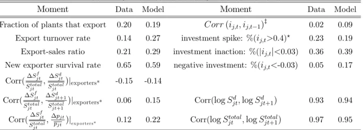
involves estimating the parameters to …t the following thirteen targets (listed in Table 1.10): fraction of plants that export, export turnover rate, mean export-to-total-sales ratio, new exporter survival rate, correlation between export and domestic sales growth for all contin-uing exporters, correlation between current export sales growth and subsequent domestic sales growth, correlation between export sales and price growth, autocorrelation of plants’ log domestic sales, autocorrelation of log total sales, fraction of plants with investment spike, fraction of plants with investment inaction, fraction of plants with negative investment, and the autocorrelation of plants’investment rate.
While there is no one-to-one mapping between individual parameters and individual statistics, certain statistics respond more to particular parameters and thus help to identify these parameters. First, identi…cation of the parameters of the capital adjustment costs function 1; 2 and 3 mainly depend on the investment and capital growth patterns at the
plant level. These parameters directly a¤ect the distribution of capital growth rate. The selling price for capital, 3, a¤ects the fraction of plants with negative investment rate. High
values of the coe¢ cient for …xed adjustment costs, 2, creates investment spikes and inaction
at the plant level. Instead, if the convex adjustment costs governed by 1 dominates, there
is more small adjustment of capital and less investment spikes and inaction. Therefore the fraction of plants with investment spikes, investment inaction and negative investment rate are informative. The auto-correlation of investment rate Corr(ijt; ijt 1) is sensitive to the
type of adjustment cost. In the absence of capital adjustment costs, the autocorrelation of investment rate is negative because of the AR(1) process of productivity and demand shocks. Under convex adjustment cost, plants adjust capital partially and it leads to a positive investment autocorrelation. It worth noting the distribution and persistence of investment rate also depend on the exogenous shock processes for demand and productivity. Second, there are parameters that governs the demand d; d and f; f, df, and those
govern the productivity processes a and a. One statistic that is sensitive to these
para-meters is the correlation between domestic and export sales growth for continuing exporters Corr( S f jt St jt ; S d jt St jt
). Productivity growth drives up sales in both the domestic and foreign mar-kets, which leads to a positive Corr( S
f jt St jt ; S d jt St jt
). On the contrary, demand growth could generate negative correlation between domestic and foreign sales growth when plants cannot freely adjust their production capacity. In addition, the correlation between plant-level price index and sales growth further helps to separate the demand and productivity process. This is because when a plant receives a positive productivity shock, its sales go up and price goes down as production cost falls. On the contrary, if a plant receives a positive demand shock, both sales and price are driven up. The target moment I use is the correlation between ex-port sales growth and price growthCorr( S
f jt
St jt
; pjt
pjt ). A positive correlation between sales and
price growth gives more weight to demand variation, while a negative one favors productivity variation. The autocorrelation for log domestic sales Corr(logSd
jt;logSjtd+1), autocorrelation
for log total salesCorr(logSjtt;logSjtt+1)are also informative about the persistence of demand and productivity processes.
Finally, the fraction of …rms that exports is very responsive to …xed exporting cost f: a lower …xed exporting cost encourages more …rms to export. The mean export-to-total-sales ratio is very responsive to the drift of the log domestic and foreign demand md and mf.
A higher mf
md implies a higher export share for exporting …rms. Export turn-over rate and
survival rate for new exporters respond to the persistence of the productivity and demand shocks: a high persistence of the shocks leads to low export turn-over rate and high survival rate for new exporters.
Table 1.10 reports the data-based statistics that the model targets to match, and their model-based simulated counterparts. The simulated model does a good job in matching the correlation between the domestic and export sales growth for continuing exporters, which represents the short-run trade-o¤ between domestic and export sales when …rms are capacity constrained. It captures the autocorrelation of log domestic sales and log total sales. It also …ts well the fraction of plants with investment inaction and spikes.
It is also worth noting that a few moments are not matched very precisely. First, there is slightly higher export turn-over rate and lower survival rate for new exporter in the simulated model than in the data. This potentially can be improved by introducing sunk export entry cost for new exporters. Second, the export-sales ratio in the model is also slightly over-predicted. This is because in the data there are a lot of …rms exporting a very small share of their output (less than 1 percent) which is not captured in the model. The correlation between export growth and price growth, and the correlation between current export sales growth and the subsequent domestic sales growth are also slightly over-predicted in the model. Finally, the fraction of plants with negative investment rate is higher in the model than that in the data.18
Table 1.11 reports the parameters associated with the estimation. The coe¢ cients for the adjustment costs imply both convex and …xed adjustment costs exist, and there is sizable gap between buying and selling the capital. These parameters are close to what Cooper and Haltiwanger (2006) obtain in calibrating their model to the U.S. economy. The implied vari-ance suggests demand ‡uctuation dominates productivity ‡uctuation in generating plants’ sales variation. This is consistent with the sales substitution patterns between domestic and exporter sales among exporters.
4.2
Simulated E¤ect of a Devaluation
I simulate …rms’ responses to a change in the exchange-rate process that depreciates the steady state value of the peso by 20%.19 It is implemented by increasing the intercept of
18While this statistics is a¤ected by the price gap between purchasing and selling the capital, it is also
a¤ected by the fraction of plants that receive negative productivity and demand shocks.
19Alternatively we can look at reduction of trade costs or increase in foreign demand. These policies would
have similar e¤ects as changes in the exchange-rate process, as the model assumes that the real exchange rate only a¤ects the e¤ective price paid by foreign consumers and thus foreign demand. Since the model does not separately identify the trade cost from foreign demand, reduction in trade cost and increase in foreign
the log exchange rate process me from 0.549 to 0.572, while keeping the persistence and
variance of the innovation term unchanged. The regime shifts take place in the middle of the sample periodtm. There are four scenarios: (I): Correctly-perceived temporary devaluation:
the currency devaluation lasts only one period and …rms have the correct expectations. (II): Incorrectly-perceived temporary devaluation: the currency devaluation lasts only one period, but …rms incorrectly perceive it as permanent. Firms correct their expectation in the following period tm + 1. (III): Incorrectly-perceived permanent devaluation: the
currency devaluation is permanent, but …rms thought it lasts only one period. They correct their expectation in the subsequent period tm + 1. (IV): Correctly-perceived permanent
devaluation: the currency devaluation is permanent, and …rms have the right expectations. Under all four scenarios the shift of exchange-rate regime was not expected before it takes place at period tm.
Short-run and Long-run Exchange Rate Elasticity of Exports
How exports respond to the exchange rate devaluation is of particular interest to this paper. The importance of capital adjustment costs in a¤ecting the export responses is re‡ected by di¤erent exchange rate elasticities of exports in the short run and long run. Its importance is also seen in how long it takes to have the export responses fully realized. Here I only focus on scenario IV where the devaluation is permanent and …rms have the correct expectations. The other three scenarios are of more interest when we look at the transitional dynamics of sales, investment and output price in the following section.
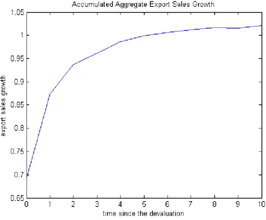
Figure 5 summarizes the transition of the accumulated aggregate export sales follow-ing the permanent shift of the exchange-rate regime. I focus on the growth rate of the accumulated aggregate export sales after the devaluation, relative to that in the base case.
b Set = 0 @X e t t=tm Stf 1 A c o u nt e r-fa c t u a l 0 @X e t t=tm Stf 1 A b a s e 0 @X e t t=tm Stf 1 A b a s e where Xet t=tm
Stf, the accumulated aggregate export sales at timeet, is the sum of aggre-gate export sales from the devaluation period tm toet:
Xet t=tm Stf = Xet t=tm X jS f jt. While
the immediate export response is big, there is still substantial adjustments in the subsequent years. The accumulated aggregate export sales increase by 70% right after the devaluation takes place at tm. The growth rate keeps rising over time, particularly during the …rst two
or three years after the devaluation. It stabilizes after about …ve years. The accumulated aggregate export sales has doubled 5 years after the permanent devaluation.
Figure 6 shows that the exchange rate elasticity of exports has increased from 2.63 at
tm to 3.46 …ve years after.20 21 Similarly, the exchange rate elasticity of exports rises fast
during the …rst three years after the devaluation takes place, and it stabilizes about …ve years after. The exchange rate elasticity of exports at et is calculated as the change of the log of accumulated export sales from the base case to after the devaluation, compared the base case, divided by the change in the log real exchange rate.
et = 0 @lnX e t t=tm Stf 1 A c o u nt e r-fa c t u a l 0 @lnX e t t=tm Sft 1 A b a s e (lne)c o u nt e r-fa c t u a l (lne)b a s e
Transitional Dynamics of Investment, Output Price, Domestic and Export sales
The e¤ects on domestic and export sales, investment and prices under each scenario, relative to a base case of no regime change, are summarized in Table 1.12. Table 1.12 focuses on the adjustments on the intensive margin (among incumbents), so it limits to the exporters that export in period tm, tm+ 1,tm+ 2 in the base case. I compare the aggregate
domestic sales for those incumbent exporters in three years following the devaluation, relative to the base case weighted by the average aggregate total sales. The change in investment is weighted by the aggregate capital. In terms of the price change after the devaluation, I look at the average price change among the incumbent exporters. Note that here the changes are year-by-year, not accumulative. The changes in domestic and foreign sales, investment and price for each scenario, in each of the three years following in the experimental devaluation
20The short-run exchange rate elasticity of exports are the same in other three scenarios, regardless the
duration of the devaluation and …rms’expectations. When the devaluation is temporary and being correctly perceived (scenario I), the long-run exchange rate elasticity of exports converges to zero because there is no export growth after periodtm.
21Here I look at export sales instead of quantity. Since there is complete exchange-rate pass through
assumed in the model, the long-run exchange rate elasticity of export quantity among export incumbents should converge to the demand elasticity.
are de…ned as: Sdt Stotal t = X j2E(S d jt)counter-factual X j2E(S d jt)base 0:5 X j2E(S total jt )counter-factual+ X j2E(S total jt )base Sft Stotal t = X j2ES f jt counter-factual X j2ES f jt base 0:5 X j2ES total jt counter-factual + X j2ES total jt base It Kt = X j2EIjt counter-factual X j2EIjt base 0:5 X j2EKjt counter-factual + X j2EKjt base pt pt = 1 N(E) X j2E (pjt) counter-factual (pjt) base 0:5 (pjt)counter-factual+ (pjt)base
In all four scenarios, at periodtm when the devaluation takes place, incumbent exporters
substitute their domestic sales towards export sales and price goes up. The aggregate export sales for the incumbent exporters increase by 18.3% compared with that the base case, while domestic sales decrease by 3.6%.The mean price has increased by 6.0%. Foreign demand increases as the domestic-produced products become cheaper for foreign consumers after the devaluation. As the marginal production cost increases on total output given the …xed amount of capital in the short run, …rms sacri…ce their sales at home to meet up the increased demand in the foreign market. It induces welfare losses for domestic consumers as price goes up.
However, …rms’investment responses It
Kt attmdi¤er depending on their perception about
the duration of the devaluation. In scenario II and IV where …rms expect the exchange-rate process to be permanent, …rms expand their production capacity in response: the aggregate investment for the incumbent exporters increase by 25.2% as a share of their total capital. In contrary, in scenario I and IV where …rms expect the exchange-rate process to move back to the base case in the following period, there are no changes in the investment level for the incumbent exporters compared with the base case.
The corresponding investment adjustment at tm in each scenario directly impact …rms’
sales and output prices in the subsequent periods, especially for scenario II and III where there is misperception about the duration of the devaluation. In scenario II, the incumbent exporters over-invest in capital at tm as they thought the devaluation is permanent while
it lasts only one period. Therefore in the subsequent period tm+ 1 as foreign demand falls
falls by 6.3%, and both domestic and export sales are higher than their counterparts in the base case. The aggregate investment decrease by 8.2% at period tm+ 1, showing that they
are reducing their excess capacity. The investment and price reduction, as well as the sales rise continue at period tm+ 2, but the magnitude is smaller. Note that the size of capital
reduction in the subsequent periods is lower than the capital expansion made in period tm,
as …rms tend to hold up to their capital in response to a negative shock because of the price gap between purchasing and selling the capital. The increased capital adjustment costs induced by over-investing and downsizing the capital afterward cause pro…t reductions for these exporters.
In contrast to the over-investment in capital in scenario II, in scenario III the incum-bent exporters under-invest in their capital as they mistakenly expect the devaluation to be temporary while it is actually permanent. As a result, the substitution from domestic sales towards export sales, and the price rise are prolonged. Firms remain to be capacity constrained in periodtm+ 1: domestic sales decrease by 3.4% at periodtm+ 1relative to the
base case. Output prices keep rising as output continues to be falling behind the demand: the mean price for the incumbent exporters’ products rise by 6.1%. This increased price leads to welfare losses for domestic consumers. As …rms correct their expectations about the duration of the devaluation in period tm+ 1, they increase their capital investment. As a
result, in periodtm+ 2, they bring back their domestic sales and price stops rising: domestic
sales increase by 2.8% in periodtm+ 2. The inadequate capital investment induced by …rms’
misperception causes pro…ts reductions for …rms and welfare losses for domestic consumers. When …rms correctly perceive the permanent currency devaluation in scenario IV, the substitution away from domestic sales for export sales is temporary. After they increase the capital investment at period tm, the incumbent exporters bring back their domestic sales
in period tm + 1: domestic sales increase by 1.9%. There is a greater response in export
sales: aggregate export sales increase by 25.3% in tm + 1, which shows that the frictions
in adjusting …rms’ production capacity generate lagged responses Price falls slightly and aggregate investment in tm+ 1 increase by 8.1% suggesting …rms make partial adjustments
in capital. In period tm+ 2 sales continue to grow, but in a smaller magnitude. At last,
in scenario I where …rms correctly perceive the temporary devaluation, the economy moves back to the base case after the temporary sales substitution and price rise at period tm.
5
Conclusion
In this paper I develop and estimate a dynamic structural model of export dynamics with capacity constraints and endogenous investment. The model features increasing marginal