Tuomas Varanka
FACIAL MICRO-EXPRESSION RECOGNITION
WITH NOISY LABELS
Master’s Thesis
Degree Programme in Computer Science and Engineering
September 2020
ABSTRACT
Facial micro-expressions are quick, involuntary and low intensity facial movements. An interest in detecting and recognizing micro-expressions arises from the fact that they are able to show person’s genuine hidden emotions. The small and rapid facial muscle movements are often too difficult for a human to not only spot the occurring micro-expression but also be able to recognize the emotion correctly. Recently, a focus on developing better micro-expression recognition methods has been on models and architectures. However, we take a step back and go to the root of task, the data.
We thoroughly analyze the input data and notice that some of the data is noisy and possibly mislabelled. The authors of the micro-expression datasets have also acknowledged the possible problems in data labelling. Despite this, no attempts have been made to design models that take into account the potential mislabelled data in micro-expression recognition, to our best knowledge. In this thesis, we explore new methods taking noisy labels into special account in an attempt to solve the problem. We propose a simple, yet efficient label refurbishing method and a data cleaning method for handling noisy labels. We show through both quantitative and qualitative analysis the effectiveness of the methods for detecting noisy samples. The data cleaning method achieves state-of-the-art results reaching anF1-scoreof 0.77 in the MEGC2019 composite dataset. Further, we analyze and discuss the results in-depth and suggest future works based on our findings.
Keywords: Affective computing, Facial expressions, Noisy data, Machine learning
TIIVISTELMÄ
Kasvojen mikroilmeet ovat nopeita, tahattomia ja pienen intensiteetin omaavia kasvojen liikkeitä. Kiinnostus mikroilmeiden tunnistamisesta johtuu niiden kyvystä paljastaa henkilöiden todelliset piilotetut tunteet. Pienet ja nopeat kasvojen lihasten liikkeet eivät olet pelkästään vaikeita huomata, mutta oikean tunteen tunnistaminen on erittäin vaikeaa. Lähiaikoina mikroilmetunnistusjärjestelmien kehitys on painottunut malleihin ja arkkitehtuureihin. Me kuitenkin otamme askeleen taaksepäin tästä kehitystyylistä ja menemme ongelman juureen eli dataan.
Me tarkastamme käytettävän datan huolellisesti ja huomaamme, että osa datasta on kohinaista ja mahdollisesti väärin kategorisoitu. Mikroilmetietokantojen tekijät ovat myös myöntäneet mahdolliset ongelmat datan kategorisoinnissa. Tästä huolimatta meidän parhaan tietomme mukaan mikroilmeiden tunnistukseen ei ole kehitetty malleja, jotka huomioisivat mahdollisesti väärin kategorisoituja näytteitä. Tässä työssä tutkimme uusia malleja ottaen virheellisesti kategorisoidut näytteet erityisesti huomioon. Ehdotamme yksinkertaista, mutta tehokasta oikaisu menetelmää ja datan puhdistus menetelmää kohinaisia luokkia varten. Näytämme sekä kvantiviisisesti että kvalitatiivisesti menetelmien tehokkuuden kohinaisten näytteiden havaitsemisessa. Datan puhdistus menetelmä saavuttaa huippuluokan tuloksen, saaden F1-arvon 0.77 MEGC2019 tietokannassa. Lisäksi analysoimme ja pohdimme tuloksia syvällisesti ja ehdotamme tutkimuksia tulevaisuuteen tuloksistamme.
Avainsanat: Affektiivinen laskenta, Kasvojen ilmeet, Kohinainen data, Koneoppiminen
ABSTRACT TIIVISTELMÄ
TABLE OF CONTENTS FOREWORD
LIST OF ABBREVIATIONS AND SYMBOLS
1. INTRODUCTION... 8
2. MICRO-EXPRESSIONS... 10
2.1. Preliminaries for Facial-Expressions ... 10
2.2. Micro-Expression Datasets ... 11
2.2.1. Spontaneous Micro-Expression Corpus (SMIC) ... 12
2.2.2. Chinese Academy of Sciences Micro-Expression II (CASME II) 13 2.2.3. Spontaneous Actions and Micro-Movements (SAMM) ... 13
2.2.4. MEGC2019 ... 14
2.2.5. Other Datasets... 15
2.3. Micro-Expression Recognition Methods... 15
2.3.1. Appearance Based Methods ... 16
2.3.2. Motion Based Methods ... 16
2.3.3. Deep Learning Methods... 18
3. NOISY LABELS ... 20
3.1. Noisy Label Methods ... 21
3.1.1. Loss Functions ... 22 3.1.2. Label Cleaning... 22 3.1.3. Label Refurbishment ... 23 3.1.4. Transition Matrices... 23 3.1.5. Loss Reweighting ... 24 3.1.6. Training Procedures... 25
3.2. A Look at the Micro-Expression Data ... 26
3.3. Proposed Methods ... 28
3.3.1. Initial Data Cleaning (IDC) ... 28
3.3.2. Loss Thresholding with Moments (LTM) ... 28
3.3.3. Iterative Label Correction (ILC) ... 30
4. EXPERIMENTAL SETTINGS ... 32
4.1. Used Models and Settings ... 32
4.2. Experimental Settings for the Noisy Label Methods ... 33
4.3. Evaluation ... 34
5. RESULTS... 35
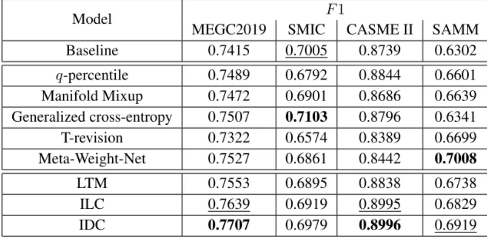
5.1. Comparison of Noisy Labels Methods... 35
5.2. Analysis of Results ... 37
5.3. Comparison to State of the Arts ... 42
5.4. Further Experiments... 42
5.5. Discussion... 44
6. CONCLUSION ... 46
This work has been done at the Centre for Computer Vision and Signal Analysis (CMVS). I would like to thank Professor Guoying Zhao for the opportunity to work in her research group and for the great support and guidance she provided during the thesis. A huge thanks also goes to Wei Peng for helping in both the technical and written side of the thesis.
Oulu, September 11th, 2020
AU Action Unit
CASME Chinese Academy of Sciences Micro-Expressions CNN Convolutional Neural Network
DNN Deep Neural Network
FPS Frames Per Second
HS High Speed
IDC Initial data Cleaning ILC Iterative Label Correction LBP Local Binary Pattern
LTM Loss Thresholding with Moments LOSO Leave-One-Subject-Out
MDMO Main Directional Optical Flow
ME Micro-Expression
MEGC The Facial Micro-Expressions Grand Challange MEVIEW Micro-Expression VIdEos in the Wild
NAS Neural Architecture search
NMER Neural Micro-Expression recognizer
OF Optical Flow
OFF-ApexNet Optical Flow Features from Apex frame Network RCN Recurrent Convolutional Network
RGB Red, Green, Blue
ROI Region of Interest
SAMM Spontaneous Actions and Micro-Movements SELFIE SELectively reFurbIsh unclEan samples SMIC Spontaneous Micro-Expression Corpus SSSNet Shallow Single Stream network
STSTNet Shallow Triple Stream Three-dimensional Network SVM Support Vector Machine
TIM Temporal Interpolation Model TOP Three Orthogonal Planes UAR Unweighted Average Recall
UMAP Uniform Manifold Approximation and Projection
C The set of clean labels
f A neural network
F N False Negative
F P False Positive
F1 F1-score
L Loss function
R The set of refurbished labels
T Transition matrix
T P True Positive
Vx Movement vector to directionx
Vy Movement vector to directiony
ˆ
y Predicted label
α Noise rate for loss thresholding with momentum
The optical strain
θ Parameters of a neural network
µ The sample mean
1. INTRODUCTION
Humans are often the subjects of many scientific studies, and even the subjects of entire fields. In the field of artificial intelligence, more specifically machine learning and computer vision, we are also interested in humans. Countless methods have been developed to recognize different properties from humans,e.g., face recognition, speech recognition, natural language understanding, recommendation systems and affective computing. Affective computing is the study of emotional behaviour of humans, including the emotional analysis of facial expressions and micro-expressions, speech and gestures—each a way of communicating non-verbally. A simple example of a facial expression is a smile, which often means that a person is feeling positive or happy about a situation. However, this is not always the case as is shown by Ekman and Friesen [1]. In 1969, the two psychologists, Ekman and Friesen, analyzed a filmed interview of a psychiatric patient. The patient seemed genuinely happy and not suicidal throughout the whole video, indicating her feelings further by using non-verbal communication in the form of a smile. However, when reviewing the tapes later Ekman found a brief segment of anguish on her face in the form of an micro-expression. It was later confirmed that she was indeed suicidal.
Micro-expressions (MEs) are rapid, involuntary and low intensity facial movements [2]. The duration of a typical ME lasts from 1/25 of a second to 1/2 of a second [2]. The intensity of MEs is very low and subtle (See Figure 2). The involuntary characteristic of an ME means that a person may perform an ME,
1. even if they are not trying to carry out any expressions
2. even if they are actively trying to hide giving away any expressions 3. even if they are unaware of expressing any emotions.
It has been shown that MEs are able to show the true emotions of a person [2], which has many applications and makes researching them particularly useful. An immediate application of MEs was shown by Ekman in the medical domain, further applications can be found from fields such as healthcare and well-being, business negotiations, security systems and marketing research [2].
The usefulness of being able to reliably recognize MEs are immense, but recognizing them has been found to be especially difficult [2]. For a person to be able to spot MEs accurately, they would have to be trained for the task. Typical humans lack the training and are thus unable to effectively detect MEs. In an attempt to make MEs more accessible, Ekman created a micro-expression training tool to train people to recognize MEs better [2]. However, the performance after training on the tool for humans was only around 50% accuracy and the training of a single person is costly. Since recognizing MEs for humans is such a difficult task, even after training, we hope to use an alternative method.
Automatic micro-expressions analysis systems use state-of-the-art techniques from machine learning and computer vision in order to reliably recognize MEs. Machine learning systems require carefully annotated data in order to perform reliably and with high performance. As MEs are difficult for even humans to spot, producing a dataset for the task is particularly difficult, as the dataset has to be labelled by humans.
Due to the characteristics of MEs (rapidness, involuntary and low intensity) not only is the data collection process difficult, but so is the process of labelling the video sequences. The characteristics of MEs make the labeling process especially volatile to mistakes. By analyzing samples from an already collected dataset we were able to find potentially mislabelled samples. In addition, the authors who created the datasets [3, 4] acknowledge the problematic labelling process and that it is prone to mistakes. Despite this no further investigations about the legitimacy of the labels or a model that is able to resolve the problem have been developed, although some papers do mention the problem [5, 6]. We hypothesize that there may be incorrectly labelled samples in the datasets, which are often referred to as noisy labels in the literature.
In recent years deep neural networks (DNNs) have achieved state of the art in many fields of computer vision, e.g., face recognition and object detection. The superior performance of DNNs has also been demonstrated in ME recognition as state-of-the-art results are almost exclusively from DNNs. Deep neural networks provide immense classification performance, so far that they are even able to fit datasets with completely random labels [7]. The testing performance is however equivalent to random assignment as the network is not able to generalize over the training data. To combat the fitting to noise, many regularization techniques have been proposed to alleviate the problem, such as dropout, batch normalization, early stopping and weight decay [8]. However, the regularization methods are often targeted to noisy data in general and not specific to label noise, which can severely reduce the performance of the system [9].
Noisy label methods have recently gained interest in computer vision [10]. Many datasets have mislabelled samples, due to the massive size of the dataset or the difficulty and ambiguity of the samples [11]. As networks are very prone to overfitting and memorizing noisy samples, techniques specific to regularizing the noise contained in labels have been developed. These methods often manipulate the loss function by weighting it, by matching the distribution of noisy and clean labels, by discarding samples or by correcting labels [11]. To the best of our knowledge there have been no previous attempts at employing noisy label methods to micro-expression recognition. Many of the noisy label methods found in the literature are however often designed for large datasets with a high percentage of noisy labels. In addition the methods are often validated on synthetically generated noise, which has been shown to be different from real world noise [12]. We thus propose noisy label methods that are capable of dealing with the challenges of micro-expressions. We propose simple, yet effective methods to find mislabelled samples and ignore the incorrectly labelled samples during the training procedure, helping the network avoid training on noisy labels.
This thesis is structured as follows. Chapter 2 introduces related work to MEs. The chapter includes preliminaries of facial-expressions, ME datasets and ME recognition methods from the literature. Chapter 3 introduces the noisy label problem, methods that have been developed to solve the noisy label problem and finally we introduce our methods for noisy labels. In Chapter 4 we give details about the implementation of the methods, the used models and evaluation, including metrics and protocols. Chapter 5 showcases the results obtained and an in-depth analysis from the results is performed. Finally we conclude the thesis in Chapter 6 by a summary.
2. MICRO-EXPRESSIONS
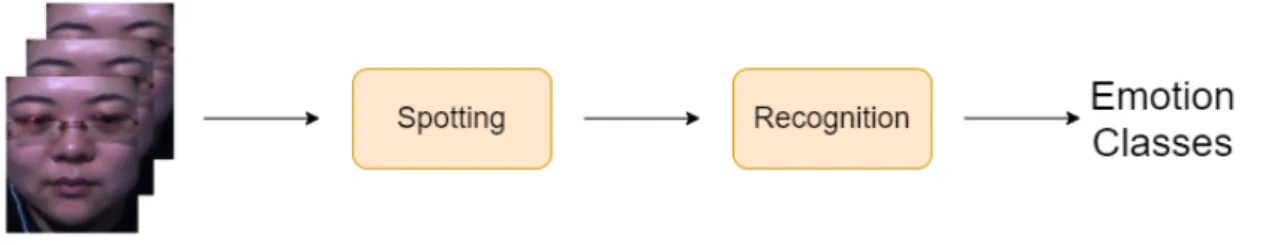
In Chapter 1 we referred to the analysis of MEs interchangeably with the terms detecting, recognition, spotting and analyzing. However, we make a distinction between those words from now on. Both spotting and detection refer to the task of finding the segment in which the ME is occurring. The starting point of an ME is referred to as theonset, while the ending point of an ME is referred to as theoffset. We also refer toapexas the point in which the intensity of an ME is at its peak. The term recognitionon the other hand refers to the classification of the segmented ME clip to its corresponding class. An automatic ME system showcased in Figure 1, consists of two tasks: first itspotsthe segment where the ME is occurring and then itrecognizes the emotion by classifying it to one of the emotion classes. These tasks are often considered separate from each other due to their complexity. This thesis will only focus on the recognition task of MEs.
Figure 1. This figure showcases a general high level view of an ME analysis system. The system takes as input a sequence of videos (left). Spotting is performed to find the subset of frames where the ME is occurring. Recognition then utilizes the information from spotting to classify the emotions to their corresponding classes. The number of emotion classes and what emotion classes are used depend on the datasets. Both of the spotting and recognition steps are typically complex systems including preprocessing and many other steps. The example frames on the left are from the SMIC (defined later) dataset and the images are shown with the permission of the authors of [13].
2.1. Preliminaries for Facial-Expressions
Facial-expressions (FEs) are facial movements that convey emotions, they can be further categorized into macro-expressions and micro-expressions. Macro-expressions typically last between 0.5 and 4 seconds and they often have a large intensity, making the spotting of them easy for humans. In fact, macro-expressions are the facial-expressions everyone is familiar with and is in contact with every day. When compared to micro-expressions, there is a clear distinction between the two. MEs only last a maximum of 0.5 seconds1, while macro-expressions go all the way to 4 seconds. The intensity of macro-expressions is large, while in MEs it is limited. Macro-expressions are mostly voluntary and they can be posed relatively easily compared to MEs, where it has been shown that posing is difficult [14]. These characteristics give us set of
1The duration of MEs is debatable, as some sources define the accepted length to be only 1/5th of a
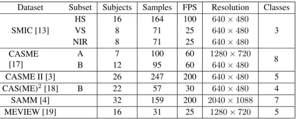
Table 1. A summary of statistics from ME datasets
Dataset Subset Subjects Samples FPS Resolution Classes
HS 16 164 100 640×480 SMIC [13] VS 8 71 25 640×480 3 NIR 8 71 25 640×480 CASME [17] A 7 100 60 1280×720 8 B 12 95 60 640×480 CASME II [3] 26 247 200 640×480 5 CAS(ME)2[18] B 22 57 30 640×480 4 SAMM [4] 32 159 200 2040×1088 7 MEVIEW [19] 16 31 25 1280×720 5
differences between the two, but in reality distinguishing between the two can be difficult.
When we think of emotions, we often think in terms of categories such as happy or sad. Formally, there are seven universal emotions: happy, sad, anger, fear, surprise, disgust and contempt[15]. How about a big smile and a small smile, how are these distinguished? Another common way to measure emotion is in terms of a continuous scale. In a dimensional emotion model, there are two axes, arousal (the level of affective activation) andvalence(the level of pleasure) that measure the extent of these values from emotions [16]. For example, both happiness and anger have similar values in arousal, but have significantly different values in valence. Continuous measurement avoids the ambiguities involved with discretizing values. However, in MEs due to the complexity and difficulty in measuring intensities, the discrete categories are commonly used instead.
Action units (AUs) are based on FACS (Facial action coding system) [2] which classify different facial muscle movements on a person’s face. For example, happiness is a combination of AU6 (cheek raiser) and AU12 (lip corner puller). AUs can be used to label images with less ambiguities as an emotion is composed of multiple smaller facial movements. However, it has been noted that in MEs this correspondence is not so straightforward [4]. Two distinct MEs with the same AUs may still be considered as different emotions due to self-reports and the content of the elicited material in the datasets.
2.2. Micro-Expression Datasets
As mentioned in Chapter 1, collecting ME data is difficult, and labeling the data correctly is an even harder challenge. Thus, a big emphasis is given to the datasets in this thesis. There are a total of six publicly available spontaneous ME datasets as of writing this thesis. Recently a composite dataset, MEGC2019 [20], was formed to provide a more generalizable way of evaluation. The MEGC2019 consists of a total of three datasets from the six publicly available ME datasets. A bigger emphasis is given to the three datasets as MEGC2019 will be used in the evaluation phase. A summary of all the datasets can be seen from Table 1 and Table 2.
First attempts at creating ME datasets consisted of posed MEs, where a group of actors tried to imitate MEs by attempting to do quick and low intensity
facial-1 (onset) 8 16 24 33 (offset)
Figure 2. Example frames from the SMIC dataset from subject one showingsurprise emotion. The numbers below correspond to the frame number. Images shown with the permission of the authors of [13].
expressions. However, the acted expressions were found to have for example different characteristics compared to spontaneous MEs [21]. Therefore, the focus has shifted towards collecting spontaneous MEs. Unfortunately, producing a spontaneous ME dataset is much harder than a dataset of posed MEs. The subjects need to be emotionally involved as acting is not enough. Emotional involvement of subjects is achieved by providing stimuli for the subjects, often through emotion inducing video clips. A high stake situation where the subjects are not allowed to show emotion is created to further increase ME inducement [13]. After collecting data comes the part we are especially interested in this thesis: labelling of the micro-expression emotion classes.
As mentioned earlier, the labelling process for MEs is difficult. First, the micro-expressions have to be detected, then the onset and offset frames have to be labelled, only after that can the emotion label be given. Different methods have been used for labelling the datasets. A convex combination of the following have mostly been used: labels based on AUs, self-report from the participant and the label from the inducing material. All the datasets used at least two of these techniques as only depending on one would be unreliable. Despite the use of a combination of different techniques, the labelling process still includes some ambiguities that could result in mislabels [4]. We will look at the labelling process of individual datasets in their corresponding sections. An important note to make is that AUs are mostly objective (label coders have some discrepancies) and the self-reports and the label from the inducing material are subjective. We hypothesize that this is one of the main reasons for ambiguities in the labels.
2.2.1. Spontaneous Micro-Expression Corpus (SMIC)
SMIC [13] was the first ME dataset that was not posed, but rather contained spontaneous MEs. It is an extension of the original SMIC-sub [22]. The SMIC-sub contains 77 samples from six different subjects recorded using a high speed camera at 100 FPS (frames per second). The extended version includes more samples as well as two more domains, a normal camera at the rate of 25 FPS and a near infrared camera
at 25 FPS as well. The extended version contains a total of 164 samples with all the samples recorded at a resolution of640×480. It only uses three classes to distinguish the emotions: positive, negative, and surprise, as they found the labelling process to be ambiguous and labelling to six different classes difficult. An example of the dataset can be seen in Figure 2. The distribution of the samples can be seen in Table 2.
The dataset does not contain labelled AUs nor the location of the apex frame, although an extended version SMIC-E [14] was published with the locations of the apex frames. The labelling of emotions was done by two annotators that compared their results with the participants’ self-reports. Only the samples in which both the annotators agreed with the participants’ self-reports were included in the dataset. The stimuli selected was the same for all the participants and no individualized selections were made.
2.2.2. Chinese Academy of Sciences Micro-Expression II (CASME II) CASME II [3] is a continuation for the CASME [17] dataset, the datasets however contain separate samples. CASME II uses a high frame rate of 200 FPS and does not contain flickering lights, as in the case of SMIC. A total of 247 samples were collected from 26 subjects. A spatial resolution of 640× 480 was also used. As opposed to SMIC, CASME II labels the emotions to five different classes: happiness, disgust, surprise, repression, andothers. The main reason for this is that CASME had a total of eight classes with some of the classes only having a few samples, so they were all put into theothersclass, to avoid an imbalanced setting.
The labelling was performed by two annotators who first marked the AUs and then determined the corresponding emotions from them. The final label is given by a combination of the AUs, participants’ self-reports and the content of the inducing material. How the combination is done exactly is not however discussed. The authors acknowledged that the labelling is ambiguous and debatable. For example a clip of chewing worms was found to be disgusting, funny or interesting for different people. Further, the two annotators had an reliability value of 84.6% when annotating the AUs. This is also a potential cause of the unreliable labelling.
2.2.3. Spontaneous Actions and Micro-Movements (SAMM)
SAMM [4] is the newest ME dataset contained in the MEGC2019, published in 2016. It has a high temporal dimension of 200 FPS, as well as a large spatial dimension of
2040×1088. SAMM improves on the distribution of its participants by having people from 13 different ethnicities and a wider distribution in the participants’ age. Having wider distributions weakens the possibilities of biases and can help create a more generalizable model. The samples are labelled based on the seven basic emotions. To prevent a problem that occurred in CASME II with some clips inducing different emotions for different people, the videos were selected personally. The participants answered a questionnaire before the experiment so that the video clips could be chosen to be more effective.
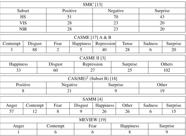
Table 2. Distributions of emotion classes from ME datasets SMIC [13]
Subset Positive Negative Surprise
HS 51 70 43
VIS 28 23 20
NIR 28 23 20
CASME [17] A & B
Contempt Disgust Fear Happiness Repression Tense Sadness Surprise
3 88 2 5 40 28 6 20
CASME II [3]
Happiness Disgust Repression Surprise Others
33 60 27 25 102
CAS(ME)2(Subset B) [18]
Positive Negative Surprise Other
8 21 9 19
SAMM [4]
Anger Contempt Fear Disgust Happiness Other Sadness Surprise
57 12 8 9 26 26 6 15
MEVIEW [19]
Anger Contempt Fear Happiness Surprise
1 6 6 8 9
The labelling is performed by three annotators instead of the typical two to ensure a more reliable result. The inter-coder reliability is 82% for AUs, slightly less than in CASME II. Unlike in SMIC and CASME II, the self-reports conducted in SAMM were done beforehand. The participants’ fears and joys were asked beforehand in order to provide them a suitable video, which was then used to label the samples. The authors also state that the focus of the dataset is on the annotated AUs and not on the emotion classes as their reliability is questionable, therefore calling the dataset not a micro-expression dataset but rather amicro-facial movementdataset.
2.2.4. MEGC2019
Due to the low number of samples in each of the datasets, the imbalanced distributions of emotions and the inconsistent evaluation protocols used by the community, a composite dataset was suggested in the second facial micro-expression grand challenge (MEGC2019) [20]. The combined dataset also evaluates the models ability to generalize over multiple different domains. Since the proposal, the MEGC2019 has been well received and is used commonly for a fair evaluation of proposed methods.
MEGC2019 consists of three datasets, SMIC, CASME II and SAMM. As all of the datasets have introduced different classes for emotions, a united set of classes had to be proposed. As SMIC has the least classes, the three classes from it were selected. The class labels from CASME II and SAMM that were labelled asrepressions,anger, contempt,disgust, fearorsadnesswere changed tonegative. The samples labelled as happiness were changed to positive. The others class from CASME II and SAMM
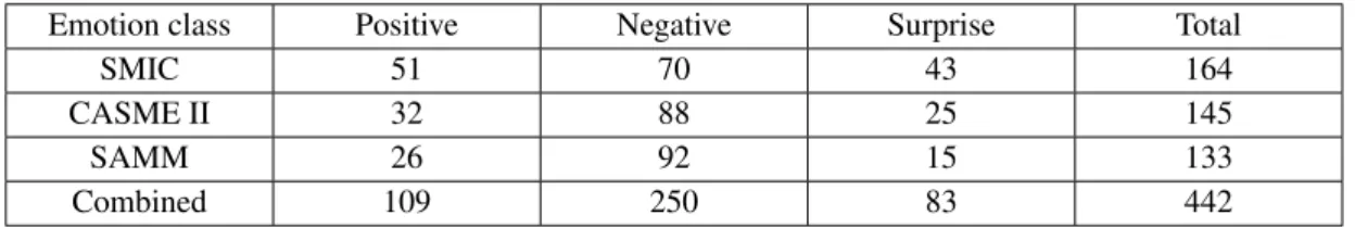
Table 3. Distributions of emotion classes for MEGC2019
Emotion class Positive Negative Surprise Total
SMIC 51 70 43 164
CASME II 32 88 25 145
SAMM 26 92 15 133
Combined 109 250 83 442
were omitted. SMIC kept all of its 164 samples; while CASME II lost over 102 samples, only keeping 145 in total; SAMM lost 26, totalling to 133 samples altogether. Thus, the new dataset consists of 442 samples from 68 different subjects with three different classes. The distribution of emotions can be seen from Table 3.
MEGC2019 is able to reduce the problem of small sample size, but even the 442 samples is still quite a low number when compared to the typical datasets used in deep learning such as CIFAR-10 [23] with 60000 samples and ImageNet [24] with more than 14 million samples. The class imbalance is also not as severe with the MEGC2019 compared to the single datasets. However, combining the datasets creates another problem: domain shift. Domain shift is the problem where the distribution of testing data differs significantly from the training data. Now that the composite dataset consists of three smaller datasets, the model may learn domain specific information which may lead to lower generalization ability.
2.2.5. Other Datasets
Other ME datasets not used in our study include: CASME [17], CAS(ME)2 [18] and MEVIEW [19]. CASME is the predecessor of CASME II which includes a total of 195 samples with a varying resolution depending on the subset. The frame rate is at 60 FPS and it includes a total of eight classes. A major reason why CASME is less frequently used is the imbalanced classes, which was later fixed in CASME II. The CAS(ME)2 is not used as commonly as it contains both macro- and micro-expressions, and the ME part only includes a total of 57 samples captured at only 30 FPS. MEVIEW is the newest dataset published in 2017 and it differs from the other datasets as the samples are not from laboratory conditions, but rather collected from online videos. As the clips are from real life situations the clips contain challenging variables, such as a changing angle from the camera and the changing lighting, providing a realistic scenario of real life challenges. The dataset also has a very small size of only 31 samples.
2.3. Micro-Expression Recognition Methods
Recognition methods in MEs are comprised of two categories as in many other tasks, from traditional methods and deep learning methods. By traditional methods we refer to methods that consist of feature extraction by a hand designed method and a classifier, whereas deep learning methods learn the feature extraction by themselves and usually the feature extraction and classification is combined. Due to the limited amount of samples in ME datasets, traditional methods have been preferred as they often require much less samples for learning, however with the development of new deep learning
techniques NNs are often the preferred choice. The main two methods for traditional methods in ME recognition can be further categorized to appearance based methods and motion based methods.
2.3.1. Appearance Based Methods
Appearance based methods use the intensity of pixel values to create features that are then used for classification. Gabor filters are a collection of different filters with different orientations and shapes. They were used by [25] for ME recognition and spotting. In [14] a histogram of oriented gradients (HGO) was used. The HOG first calculates the gradients of the image for blocks, which are then transformed to the polar coordinates. A histogram is then created by quantizing the direction, and the value for each bin is then created by the sum of magnitudes of gradients.
Local binary pattern (LBP) is a texture descriptor that calculates a feature vector by thresholding the neighboring pixels in a circular area from divided blocks from an image. Since MEs occur both in the spatial and temporal domains, a dynamic feature extraction method is required. To capture the temporal domain as well as the spatial domain an extended version of the LBP is used, local binary pattern from three orthogonal domains (LBP-TOP) [26]. As the name suggests LBP-TOP calculates the LBP from three different planes, the planes being XY, XT and YT. Here X and Y refer to the x-coordinate and y-coordinate in an image, and T to the time dimension,i.e., the video length. Only calculating the XY planes would result in the original LBP.
LBP-TOP was used as the baseline in the first spontaneous ME dataset, and has since become a stable baseline for comparison as well as inspired many variants [27, 28, 29]. In [13] a temporal interpolation model was used to both downsample and upsample the samples to have an equal number of frames, after which the LBP-TOP was used for feature extraction, finally the features were then classified using the support vector machine. LBP-SIP (local binary pattern - six intersection points) [27] only uses the six intersection points unique in the different planes to reduce the computational cost. LBP-MOP (local binary pattern - mean orthogonal planes) [28] uses the mean of the three different planes instead of the individual frames to reduce computations and redundant information. Extended LBPTOP (ELBPTOP) [29] uses the second order information from radial and angular differences to include extra information.
2.3.2. Motion Based Methods
The second type of commonly used traditional method in ME recognition is based on the optical flow. We first define the optical flow (OF) precisely as it is used extensively throughout our analysis. OF is used to measure the difference between two sequential images. The brightness constancy constraint
tells us that the intensity of an image I(x, y, t) stays constant throughout different time steps. The intensity change ofI(x, y, t)at pixel(x, y)at timetcan be thought as adding the movement∆xand∆yin duration∆t. By assuming the movement is small, equation (1) can be constructed with the Taylor series by linearizing the right side
∂I ∂xVx+ ∂I ∂yVy+ ∂I ∂t = 0, (2)
whereVxis the movement inxdirection and similarlyVyis the movement inydirection
[21]. Equation (2) is problematic since we have two unknown variables and only one equation. Different methods for approximating optical flow have been developed. A simple method is to assume that the neighboring points share the same changes of Vx and Vy—this changes the problem to an overdetermined linear system which
can be solved easily by least squares [30]. More advanced techniques that use less assumptions and perform better have been developed. In this thesis the OF method used is described in [31].
In addition to the[Vx, Vy]components we can calculate the optical strainfor second
order information [32]. The optical strain is defined as = 1
2[∇V + (∇V)
T], (3)
whereV = [Vx, Vy]. The optical strain is the gradient of the OF components, which is
able to give more detailed information by disregarding noisy parts. Methods
The first use of OF in ME recognition was by histogram of oriented optical flow (HOOF) [33, 21]. HOOF calculates the movement vectors in the Cartesian coordinates
[Vx, Vy]and transforms them to the polar coordinates[ρ, θ]. The orientation directions
are then placed to bins and the magnitudes corresponding to the orientations from each of the bins are summed together. The bins can then be used as feature vectors. Main directional mean optical flow (MDMO) [21] improves HOOF by introducing regions of interest (ROIs) from which the histograms are calculated. The 36 ROIs were carefully constructed to include most of the AUs in such a way that one ROI would correspond to one AU. MDMO reduces the number of bins by only choosing the bin with the maximum number of vectors and then calculates the mean vector from that. SparseMDMO [34] avoids losing structure by aggregating over the frames, and instead uses all histograms from all frames. This however increases the length of the feature vector, which is then made sparse by using graph sparse coding [35] to reduce the feature vector to only include the important features. Bi-weighted oriented optical flow (Bi-WOOF) [36] takes a slightly different approach by only using the onset and the apex frame of the sample. In addition to using the[Vx, Vy]components, Bi-WOOF
2.3.3. Deep Learning Methods
Many recent methods in ME recognition have started to adapt deep learning into their methods [37, 15, 38, 39, 32, 40, 41, 42]. As with most computer vision tasks, ME recognition also uses convolutional neural networks (CNNs). Due to the temporal component of MEs, a sequential model is required to model videos, such as long short-term memory networks (LSTM). A combination of LSTM and CNN was developed in [15]. However these methods require a large number of parameters, which is something that should be avoided with small scaled datasets. Instead, the finding from [36] of only using the onset and apex frame was adopted—thus only requiring the use of a typical CNN. One of the first uses of CNNs on only the apex was in [38], where the authors fine-tuned a VGG-face on the apex, where motion of the experessions had been magnified by a Eulerian magnification method. In addition, they used the neighboring frames of the apex in the training phase to include more data.
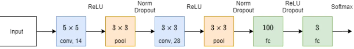
One of the first approaches of using a CNN on OF inputs was the work from optical flow features from apex frame network (OFF-ApexNet) [39]. The OF is able to capture the major movements, reducing the need for multiple frames and even the need for high resolution inputs. In OFF-ApexNet, a network with two convolutional streams is provided for each of the input components [Vx, Vy]and then the learned features are
concatenated to fully connected layers for prediction. The inputs are reshaped to a size of only28×28, to reduce the computational complexity and the number of required parameters. The network consists of two convolutional layers with max pooling at the end of each stream and three fully connected layers for classification. Shallow triple stream three-dimensional CNN (STSTNet) [32] has a similar architecture to OFF-ApexNet, but only uses a single convolutional layer and a single fully connected layer, which drastically reduces the number of parameters. The input is changed to include the optical strain[Vx, Vy, ], increasing the number of streams to three.
An RCN (recurrent convolutional network) was employed in [40], as the result of finding that shallower lower complexity models perform better in ME recognition. In addition, it was found that the input size should also be relatively small (60× 60), allowing to further decrease the number of parameters. The authors also developed three independent hyperparameter-free modules for the RCN: wide expansion, shortcut connection and attention unit. To find the best combination and location of the proposed modules, a neural architecture search was performed but the results did not improve over just having the individual modules.
To compensate for the lack of data, NMER (neural micro-expression recognizer) [41] proposes to increase the dataset by including data from a macro-expression dataset. Due to the difference between macro- and micro-expressions, two domain adaptation techniques are applied for the model to take full advantage of the extra data. As input data for the MEs, the raw frame from the apex is used. For the macro-expressions the middle frame between the onset and the apex is used to simulate the lower intensity of MEs. To maximize the similarities between the two domains a motion magnification method is used on the MEs. Adversarial domain adaptation is used in the training process to encourage domain-independent features. However, the model only performs at the level of LBP-TOP, possibly due to the innate differences between macro- and micro-expressions.
To compensate for the lack of data, [42] uses a GAN (generative adversarial network) to create more data. Due to the complexity of the raw data, only the optical flow is used. They experimented with two types of GANs: auxiliary classifier GAN and self-attention GAN. However, the performance of the models only decreased with the generated data. We hypothesize that since the GANs are used independently of the classifier they are optimizing for the images ability to look natural. However, this is not optimal as shown in [43], instead the GAN should be optimized in an end-to-end manner with the classifier such that the generated images are optimized for the classification task at hand.
3. NOISY LABELS
As machine learning is being presented with more and more tasks, it is also being introduced to more difficult tasks. Some of the tasks can be so difficult that even a human is not able to consistently perform well on them. This can make the labelling process of a dataset a demanding task, which is a crucial step as typical machine learning systems require well annotated large scale data. The difficulty of the tasks may be due to the innate ambiguity of the samples, the samples being borderline cases or the samples having multiple correct labels. Examples of tasks that contain difficult samples are many medical imaging problems such as segmentation of brain lesion [11] and of course micro-expressions. As annotators are labelling the data, the ambiguous data may lead to mislabelled samples, which we refer to as noisy label samples. These are different from samples where the noise is contained in the input data. A simple example of a noisy label is an image of a cat that has been labelled as a dog.
The recent success of deep learning has led to its widespread usage over many different tasks in machine learning, computer vision and even outside of these fields. One of the reasons is their incredible representation power. It was even shown that deep learning models are able to fit datasets with completely random labels [7]. Due to the powerful representation ability of DNNs, the incorrect labels can be detrimental to the training process compared to traditional machine learning methods [9]. To prevent DNNs from overfitting to the training set, various regularization methods are used: dropout, batch normalization, weight decay and early stopping [8]. However, these methods are meant for overall regularization of noisy data, and are not specifically designed to solve the problem of noisy labels. Thus an interest in developing noisy label methods that are able to regularize incorrect labels have surged recently [10]. The basic idea of noisy label methods is to regularize the effects of incorrectly labelled samples during the training process.
We divide the noisy label tasks in the literature to two different categories:
1. Large scale datasets created by non-experts or automated systems. One of the thriving forces of the success of deep learning can be attributed to the existence of large datasets. Creating a large dataset is desirable as it can increase the performance of models significantly [11]. However, the datasets have to be carefully annotated. To achieve this, multiple annotators are often used to avoid mistakes [11]. Using multiple annotators on a large dataset can however be expensive and thus cheaper alternatives have been sought [11, 44]. One solution is to use non-expert humans to annotate the dataset. Another, even cheaper solution is to use automated methods with little or no human supervision at all. An example of this is Webdata [11], which is created by using an internet crawler that annotates the data based on information around the data. Although these methods are cheaper alternatives than using multiple annotators, the labelling methods often suffer from high label noise.
2. Difficult and ambiguous data. This type of data is inherently difficult or ambiguous even for humans. The datasets are typically relatively small allowing it to be annotated by multiple people, but they can still contain noisy labels due to the difficulty of the data. In the previous section the datasets typically consist of images that are natural to humans, like animals or vehicles, but in this category
the data is not only difficult for non-experts but even for experts. The data can be ambiguous by being noisy, being a borderline case in between two classes or the sample may have multiple different labels that are all correct. Example datasets are medical images that require healthcare professionals trained for the task, and micro-expression data that also needs professional FACS coders and is not entirely objective. Due to the smaller size and the use of experts these datasets often have fewer mistakes compared to the automatically annotated datasets. Based on [11] and [44] the two tasks seem to have slightly different methods, although the difference does not seem to be discussed frequently throughout the literature. Large datasets obviously have the advantage of having numerous training samples, which allows the use of larger models, validation data and the use of clean data (due to the simplicity of the data). Due to having numerous samples from which to learn, the discarding technique shown in Figure 5 can be used without necessarily dropping important samples that are crucial for training. In smaller datasets, discarding even a few samples can significantly affect the training negatively. Some datasets may also contain higher levels of noisy labels and thus require methods that are able to perform even with extremely high label noise.
3.1. Noisy Label Methods
We formally defined the noisy label problem here. LetX ⊆Rdbe the space of inputs
and the spaceY ={1, . . . , c}be the label space, wheredis the dimension of the inputs andcis the number of classes. In a typical case we hope for the training set to consist of clean tuples of(x, y)∈ (X,Y), but in a noisy label case we have(x,y˜) ∈ (X,Y˜), whereY˜is the set of noisy labels. The clean and noisy labels are related by a function g : Y → Y˜, that maps the clean samples to noisy samples. The task of noisy label methods is to try to undo the mapping, i.e., find g−1. However this is an ill-posed problem and only approximate solutions can be found. One set of methods tries to modelg−1on a class level by creating an error transition matrixT
ij =p(˜y =j |y =i).
Other methods settle for implicit solutions by discarding samples with noisy labels or refurbishing them through predictions.
Various methods have been proposed for learning with noisy labels, especially recently [10]. A small proportion of the methods were developed for traditional machine learning methods, which we will not cover. Due to NNs ability to fit noisy datasets, the problem of noisy labels is much more prevalent in deep learning methods than in traditional machine learning. We categorize the following subsections based on classification of the methods found in the literature inspired by [44, 11]. We deviate slightly from the categorization in the literature to better suit and emphasize the most important categories for ME recognition.
Before going into the methods we describe a crucial finding that is commonly used throughout the different methods, named as thesmall-losstrick by [44]. The loss of a single sample is determined by the DNNs prediction. For example, the frequently used categorical cross-entropy −P
n∈N ynlog(ˆyn) measures the difference between two
distributions, whereN is the set of possible classes. If the distribution of the predicted labelyˆis similar to that of the real labely, the loss will be small. If the distributions are
different, then the loss will be high. For representative and unambiguous clean samples we would expect the loss to be small at the end of the training. For difficult clean samples the loss may be high as the network is not able to fully match the distributions. For samples with noisy labels we expect the loss to be high, as the network is predicting a distribution that does match the real label’s distribution.
3.1.1. Loss Functions
The methods in this category are relatively self-explanatory, they simply change the loss function used to optimize the network. Mean absolute value of error (MAE) [45] uses the `1 norm to calculate the loss as opposed to the typical cross entropy. The idea is similar to performing regression using `2 and `1 norms, where the `2 weighs outliers heavily, while `1 keeps the weights equal for all samples. The use of MAE makes intuitive sense as samples with high loss values can be thought of as outliers or as samples with noisy labels in our case by the small-loss trick. However, the MAE loss can also discard clean samples that have a high loss, due to the samples merely being difficult, hindering the network’s performance. A modified version that contains both the good qualities of MAE and cross-entropy was proposed to create a generalized cross-entropy by using a negative Box-Cox transformation [46]
Lk f(x),yj
= 1−fj(x)
k
k .
The authors in [46] show that the loss is equivalent to cross-entropy whenkapproaches
0and MAE when k = 1. Then we can choose ak, such that0 < k ≤ 1, to have a combination of the cross-entropy and MAE losses in order to have both the benefits of MAE and cross-entropy.
3.1.2. Label Cleaning
Label cleaning methods attempt to identify samples with incorrect labels before or during the training and either discard them or ignore their gradients during the training. One of the more intuitive ideas is to use the loss of a sample as an indicator based on the small-loss trick. Samples with high loss values are either discarded or ignored during the backpropagation and their gradients are not updated, while samples with small loss values are kept. One of the downsides of this method is that one has to define what is considered as a high loss value, which is dependent on the data. Frequently the notion of q-percentile is used, here q percent of the data is assumed to be noisy, and only the (1 − q)% is kept. The losses of a batch are sorted and q% of the highest values are discarded from updating their gradients. One of the downsides of q-percentile is the need for a warm-up, as the small-loss trick does not apply during the early stages of training. Nonetheless, the method is used by multiple works [11, 47, 48, 49] as either the primary method or as a part of a more complicated method. Another very intuitive idea is to use the network’s predictions as a thresholding mechanism. Rank pruning [50] uses the confidence of the network
predictions (after the softmax layer) as an indicator whether the sample is noisy or not. This method makes the assumption of well behaving classification borders or "well calibrated" network [11]. A well calibrated network’s predictions should match the likelihood of it being correct. However, this is often not the case as shown in [51, 52]. Networks frequently tend to be overconfident of their predictions, which makes this method reliant on the networks calibration level. CleanNet [53] uses a strategy that compares the feature representations of samples with noisy labels to samples with clean labels and then uses the similarity between the samples to determine whether the sample is kept or discarded. This method requires a clean subset of the data that can be used to create the clean feature representations.
An important thing to note is that all of the methods in this category can also be used to reweight the samples. Each of the samples can be given a weight instead of thresholding, samples with noisy labels should be given a low weight. The weights can be used to construct a sampling distribution which is used for sampling the data during training. Alternatively, the weights can be used to weigh the loss values, affecting the length and direction of each gradient step.
3.1.3. Label Refurbishment
Label refurbishment methods assign new pseudo labels to the samples, instead of completely discarding them. Correcting a label can however be risky—one may end up with more noisy labels than they started with if the corrected labels are wrong. The corrected pseudo label is attained by a convex combination λy˜+ (1 − λ)ˆy of the noisy label y˜and a predicted label y. In [54] the authors use a static coefficientˆ
for the convex combination and find it through cross-validation. Different methods have been proposed to determine the coefficient of the convex combination. Note that the coefficient can be unique for each sample and it can be adaptive throughout the training. Dynamic bootstrapping [55] uses this idea and estimates the coefficient for each sample for every epoch using a beta mixture model, which measures whether the sample belongs to the distribution or not. The method is built around the idea that loss distribution often takes the shape of a beta distribution with clean data. SELFIE (SELectively reFurbIsh unclEan samples) [48] uses the simple idea that not all samples have to be refurbished. SELFIE first uses the basicq-percentile strategy to find samples with high loss values and discards them unless they satisfy the refurbishable condition. The refurbishable condition is met if the sample’s predictions from the network are consistant. Formally the condition is given by the normalized entropy of the predicted values and a thresholding value. If the label satisfies the condition, its label is corrected by using the most frequent prediction from the network. SELFIE uses a λ = 0 and only uses the predictionyˆfor the pseudo label.
3.1.4. Transition Matrices
Transition matrix methods modify the loss function or the predicted labels by multiplying it with the inverse transition matrix T−1 (defined in Section 3.1) in an attempt to make the distributions of the network’s predicted probabilities match the
distribution of noisy labels. The idea was first proposed by [56] and they proposed to learn the transition matrix by adding the transition matrix as a linear noise layer to the end of the network and then backpropagating through it. To make the model converge, the authors use a trace norm of the transition matrix for regularization. Clean data can also be used to improve the estimation of the transition matrix. Backward correction [57] decouples the estimation of the transition matrix from the model and estimates it using either clean data or by using a pre-trained network. The pre-trained network gives the probabilitiesp(˜y| x)for each class, which can be then used to construct the estimated transition matrixT.ˆ
Often datasets are labelled by multiple annotators and their inter-observer variability tells how well the annotators agreed with each other. A work by [58] shows that utilizing all the different sets of labels from different annotators leads to better performances compared to just using an aggregated version of the collection of labels. The authors estimate a confusion matrix for each annotator to model the true label distribution. Each of the confusion matrices are used with the noisy prediction to create a clean prediction for each annotator. The loss is then calculated as the sum of all the different predictions. Similarly to [56] a trace norm is used to regularize the transition matrices. In addition [11] experimented with the method on a task of prostate cancer digital pathology classification achieving the best result compared to just using a single annotator or a majority vote between the annotators.
More recently, T-revision [59] shows that clean samples are not necessary for the optimal learning of the transition matrix T. They use the same idea as [57] of using the posterior probabilitiesp(˜y | x)to estimateT. However by only utilizing the noisy class posterior probabilities the transition matrix is often estimated poorly. As clean samples can significantly estimate T better, the authors propose to use samples that are likely to be clean. They determine the clean samples to be the ones with a high predictive value from the network. After the initial estimations of T, revision are made by adding a slack variable∆T to the initial estimationT. Their proposed riskˆ function is asymptotically equal to the risk function with clean data, ensuring accurate estimation.
3.1.5. Loss Reweighting
Loss reweighting attempts to give larger weights to clean samples and smaller weights to noisy labels in the loss function. Unlike methods like focal loss, AdaBoost and hard negative mining that give more weight to hard samples, the opposite is wanted in noisy label learning based on the small-loss trick [60]. Self-paced learning uses a decreasing weight function for the loss, giving more weight to samples with lower loss. However, this method requires a hyperparameter and the piecewise linear weighting functions may not be optimal for the used data. Thus, a multilayer perceptron is used to model the weighting function [60]. The weighting function is learned through a clean meta dataset. The authors show its ability to create complex weighting functions for different datasets. As the method models the weighting function, it can be used for both noisy label problems, as well as imbalanced data that requires the weights to be higher for high loss samples. The work from [47] uses an outlier detection method to weight the samples. Probabilistic local outlier factor (PLOF) gives a value between 0
and 1 whether the sample is an outlier or not and the authors use this value directly to weigh the samples. Conversely to thresholding, these methods can also be used for data cleaning, by setting a threshold value from the weights.
3.1.6. Training Procedures
Curriculum learning is a training strategy where a curriculum is created for the incoming data. The idea is natural to human learning—we start by learning easier things and then move to progressively harder tasks. Currently, most networks simply use a random order and the network might start learning difficult samples immediately. Although the idea of curriculum learning is often synonymous to starting with easier samples and moving to harder samples later on in the training, the idea can be generalized to creating an arbitrary curriculum that may in fact do the opposite. Another common strategy is to first train on "important" or representative samples, which is similar to the idea of easy samples. In [61] the authors design methods that are able to find representative samples, these samples are then used to create a ranking of the most representative samples which is then used as the curriculum.
Similar ideas have been used in noisy label methods as well. The idea is to rank the confidence level of each sample being a clean label and use the ranks to create a curriculum, the clean samples should be used first in the training and the incorrect labels later. MentorNet [62] uses a teacher network to guide the training of a student network by providing it a curriculum that is learned with an LSTM network. The curriculum is learned by using a small clean dataset. CurriculumNet [63] uses a clustering technique to find samples that are likely to have noisy labels. They cluster the data in a feature space provided by a pre-trained network and then sort the samples based on their local density to obtain the curriculum. This method is especially designed for massive web data, with heavy noise in addition to imbalanced data.
In sample selection the target is to select a subset of the minibatch that only contains the clean samples. Decouple [64] uses two networks and only updates the samples that have different predictions between the two networks. For easy clean samples the predictions of the two networks should match as both the networks will likely be able to predict the correct label. For noisy label samples the networks should also agree, the prediction is likely to be wrong, but both the networks agree. For difficult, near the decision boundary samples, the predictions could differ from the networks. With this strategy the networks are able to ignore the noisy labels and train using the difficult samples at the later stages of training.
Mixup [51] is not directly a noisy label method, but an overall regularization method. However, it has been observed to work as a regularizer for noisy labels as well [11]. Mixup works by synthesizing new labels using a convex combination of samples. Both the input data and the labels are combined as Xmix = λXi + (1−λ)Xj andymix =
λyi + (1 −λ)yj, giving a soft label for the new sample. An extension of the work
named Manifold Mixup [52] expands the use of convex combinations to include hidden layers as well. Both the methods have also been shown to improve results for domain generalization and zero-shot learning [65], demonstrating their capability as effective regularizers.
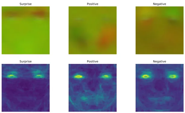
Surprise Positive Negative
Surprise Positive Negative Mean images from all subjects
Figure 3. Mean of the optical flow aggregated based on the emotion class. Top: The three channels from OF[Vx, Vy, ]. The movement is shown in red. Bottom: Only the
optical strain channelis displayed for clarity. The movement in shown in green and yellow.
3.2. A Look at the Micro-Expression Data
This section will provide a qualitative analysis of the ME data, where we will look at the the OF (optical flow) between the onset and the apex frame from the samples in the MEGC2019 dataset. Each sample consists of three channels: the horizontal component of OF, the vertical components of OF and the optical strain denoted by[Vx, Vy, ].
Figure 3 shows the mean samples of each emotion class. The surprise emotion has mainl movement on the forehead and eyebrows. ThePositive emotion mainly has movement on the left (from the participant) cheek. By looking at the optical strain the movement seems to be on both cheeks and the mouth area. TheNegativeemotion does not seem to have any distinct movements, there are some movements around the eyebrows, but also near the mouth. We believe this is due to the aggregated classes, as the MEGC2019negativecontains multiple other subclasses. The eyes are highlighted on all the classes due to blinking. We will use these distinct movements of each class to search for any inconsistencies in the dataset.
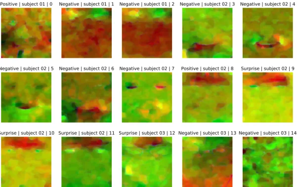
Figure 4 shows the first 15 samples of MEGC2019. Starting our observations with the sample zero located at the top left of the figure, we can immediately see that it is very noisy. By carefully inspecting it we are able to see some movement on the left cheek, which seems to correspond to the movements we saw in Figure 3 for thepositive class, making the label for this sample likely to be correct. The next two samples, numbers one and two, are very similar and both seem to be quite noisy. Movements can
Positive | subject 01 | 0 Negative | subject 01 | 1 Negative | subject 01 | 2 Negative | subject 02 | 3 Negative | subject 02 | 4
Negative | subject 02 | 5 Negative | subject 02 | 6 Negative | subject 02 | 7 Positive | subject 02 | 8 Surprise | subject 02 | 9
Surprise | subject 02 | 10 Surprise | subject 02 | 11 Surprise | subject 03 | 12 Negative | subject 03 | 13 Negative | subject 03 | 14
Figure 4. First 15 samples of MEGC2019. The title of each image consists of the emotion class|the subject number|the sample number.
be seen essentially everywhere below the eyes. These samples do not fit our description of positiveas the movement is further spread from the cheeks orsurprise as there is only small movement on the right eyebrow, therefore the classnegativemakes sense. Next, the samples three, four and five also contain many similarities with each other. These emotions are allnegative, but they do not look anything like the samples one and two. This is due to the samples having a different subclass as thenegative emotions were aggregated to one in MEGC2019.
An interesting discovery can be made from the samples eight, nine, ten and eleven. All of these samples look similar but one of them is labelled aspositivewhile the others are labelled as surprise. The sample number eight also contains some movements on their cheeks which may have been the reason for the label positive, but so does sample number ten and it has not been labelled as positive. This is a great example of an ambiguous sample, where there could even be two correct labels, as the sample contains two distinct movements for two different emotions. However, confirming that this sample has a noisy label is difficult as we do not have an expert to confirm the finding and since this is only the apex of the OF, many more things could be happening in the other frames in the original domain. Nevertheless for the model performing the classification this sample will most likely be classified assurprise due to the distinct movements in the forehead. We find more similar samples by going through the dataset and hypothesize that these are samples that have been labelled incorrectly.
3.3. Proposed Methods
This section introduces three methods for noisy label learning: initial data cleaning (IDC), loss thresholding with moments (LTM) and iterative label correction (ILC). IDC and LTM are similar to each other as they both discard samples, but the way the discarded samples are chosen is fundamentally different. As IDC is not able to generalize to larger datasets we also introduce two automatic methods that are able to scale. ILC essentially extends LTM by not discarding the samples, but instead by correcting the labels. We develop new noisy label methods as many of the methods found in the literature have been developed using synthetically generated noise, which has been found to be different from real world noise [12]. This hinders the methods’ ability to perform on real world datasets like the ME datasets. In addition, our task is harder in the sense that we have no clean validation set.
3.3.1. Initial Data Cleaning (IDC)
It was found in [11] that only using clean data (10% of the full data) can lead to a better performance than using the whole dataset, including the noisy samples. Inspired by this we manually go through the dataset to find clean samples similarly to the previous section. From the 442 samples of MEGC2019 we find a total of 240 clean samples and 202 samples that are noisy, have a potentially incorrect label, ambiguous or do not fit the typical characteristics of MEs found in the previous section. The number of noisy samples is so high because we use a high threshold in determining clean samples. However, after experimentation we found that the performance had decreased when only training with the clean samples. A finding in [44] points out that data cleaning methods may be cleaning too many samples, discarding samples that are crucial for the training. In the work [66] the authors find that regularizing the network early significantly prevents the network from memorizing the noisy labels in the later stages of the training. Inspired by this we propose a warm-up period during which the network is only trained with clean labels for some duration of epochs, hence the data cleaning is only done initially. After the warm-up period the network has access to all of the data, including the samples with noisy labels, allowing access to potentially important samples.
3.3.2. Loss Thresholding with Moments (LTM)
We introduce loss thresholding with moments here as it is used as a sub method in ILC. We use an alternative way of performing theq-percentile also based on the small-loss trick. One of the downsides of q-percentile is the need for a warm-up period as the small-loss trick does not apply at the beginning of the training when the losses are essentially random. In [11] the authors propose to store the mean µand standard deviationσof the losses of the most recent 100 training samples. Then they threshold the values if the loss value is higher than µ+ 1.5σ. We use the same idea but set the coefficient to be a hyperparameterα, thus the threshold value is then given by
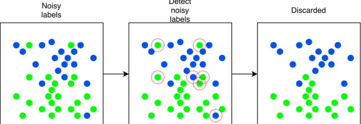
Discarded Noisy labels Detect noisy labels
Figure 5. The figure depicts loss thresholding with moments. (Left) We start with a set of noisy labels. (Middle) We detect the noisy labels using the threshold valuetgiven in Equation (4). (Right) The samples that exceed the threshold value tare discarded and we are left with the clean setC given by Equation (5). LTM leaves us with clean, but fewer data points that are then used to update the model.
t =µ+ασ. (4)
The hyperparameterαbehaves similarly toqand is required as different datasets have different levels of noise. The number of training samples from which the mean and standard deviation are calculated is set to be equal to the number of samples in a batch. This allows us to perform an update based on the most recent loss values and have enough samples to calculate the moments. In addition, by calculating the moments from the batch samples we can avoid more complex implementations. The value may have to be adjusted depending on the size of the dataset and if the ratio of noisy labels is small. We name the method loss thresholding with moments (LTM) as we use the first and second moments of the distribution to formulate the threshold value.
The set of clean labels
C ={(x, y)∈(X,Y)| L(f(x;θ), y)< t} (5) is then obtained by thresholding the loss values obtained from an arbitrary loss function
L of each sample, where the networkf gives the prediction. Then, the samples with high loss values are ignored when updating the parameters of the networkθ and only the set of clean samples is used in the update with a learning rate ofγ. The update for the parameters is then given by
θ:=θ−γ∇ 1 | C | X (x,y)∈C L(f(x;θ), y) .
The benefit of using LTM over q-percentile is that there is no need for a warm-up period at the start of the training. As the threshold valuetis given as a function of the moments of the loss distribution, the number of discarded samples is adaptive. Later in Section 5 we show that LTM does not require a warm-up period to work. The method belongs to the class of data cleaning and the process is shown in Figure 5.
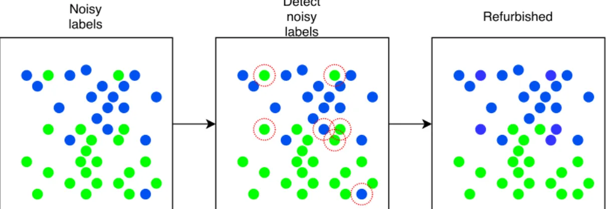
Refurbished Noisy labels Detect noisy labels
Figure 6. The figure depicts Iterative label correction. (Left) We start with a set of noisy labels. (Middle) We detect the noisy labels similarly to LTM. (Right) The samples that are detected as noisy labels are refurbished by the network’s most recent prediction and we are left with the clean setC and the corrected setRgiven by Equation (6). By correcting the labels we are left with the same amount of samples that we started with.
3.3.3. Iterative Label Correction (ILC)
An issue with LTM, and overall with methods discarding samples, is that the discarded samples may be important for the training in small datasets. Therefore we would like to use a label refurbishing method. As discussed in Section 3.1.3, SELFIE uses the idea that not all samples have to corrected, but only the ones we are uncertain of. Our method is similar to SELFIE, but it differs in a few points. Firstly, for the base method of choosing the high loss samples which will be refurbished, we use LTM,i.e., Equation (5), while SELFIE usesq-percentile. Secondly, SELFIE also corrects some of the labels of samples that had been confirmed clean by the cleaning process, while we only correct the label if it is considered to be a high loss sample. The corrected label is determined similarly but we simplify and use the current prediction of the network compared to the most common prediction over some period of time used by SELFIE, as the network could have recently learned something new, making the most recent prediction the most reliable. The set of corrected labels
R={(x,yˆ)|(x, y)∈ Cc, yˆ=f(x;θ)} (6)
is then given by the predictions of the network for samples that were not found to be clean,i.e.,, the complement ofC. The parameters are then updated using both the clean setC and the corrected setRby
θ :=θ−γ∇ 1 | C ∪ R | X (x,y)∈C L(f(x;θ), y) + X (x,ˆy)∈R L(f(x;θ),yˆ) .
Like SELFIE, ILC also requires a warm-up period as the predictions from the network would not be reliable at the beginning of the training. Algorithm 1 describes the process of ILC for a single epoch and Figure 6 illustrates the method.
The correction of labels can be risky however. If the network has not learned the dataset correctly it is not able to distinguish between the samples and the corrected labels may be incorrect. Giving the high loss samples incorrect labels could lead to an
increase in the number of noisy labels. One of the bigger benefits of using LTM instead ofq-percentile is that we can start discarding the samples already in the warm-up phase as seen in Algorithm 1. This mitigates the possibility that the network will overfit to the noisy samples later in the training [66].
Algorithm 1. Iterative label correction
Input :A datasetD, noise levelα, warm-upγ, current epochi, neural networkf.
1 #Draw a batch 2 for(X,y)∈ Ddo
3 yˆ=f(X;θ)#Network’s prediction 4 ` =L(ˆy,y)#Vector of losses
5 t =µ+ασ #Use`to calculate the threshold value by Equation (4) 6 C ={(x, y)∈(X,Y)|`< t}#Set of samples with clean labels 7 ifi < γthen 8 #Warm-up 9 θ :=θ−γ∇ 1 |C| P (x,y)∈CL(f(x;θ), y)
#Update parameters only from clean samples
10 end 11 else
12 R={(x,yˆ)|(x, y)∈ Cc, yˆ=f(x;θ)}#Set of noisy samples with
corrected labels
13 #Update parameters from both clean and corrected samples 14 θ :=θ−γ∇ 1 |C∪R| P (x,y)∈CL(f(x;θ), y) + P (x,yˆ)∈RL(f(x;θ),yˆ) 15 end 16 end