Model Fusion for Building Type Classification from
Aerial and
Street View
Images
Eike Jens Hoffmann1, Yuanyuan Wang1, Martin Werner2, Jian Kang1, and Xiao Xiang Zhu1,2* 1 Signal Processing in Earth Observation, Technical University of Munich
2 Remote Sensing Technology Institute, German Aerospace Center
* Correspondence: [email protected] Version June 26, 2019 submitted to Remote Sens.
Abstract: This article addresses the question of mapping building functions jointly usingbothaerial
1
andstreet viewimages via deep learning techniques. One of the central challenges here isdetermining
2
adata fusion strategy that can cope with heterogeneous image modalities. We demonstrate that
3
geometric combinations of the features of such two types of images, especially in an early stage of the
4
convolutional layers, often lead to a destructive effect due to the spatial misalignment of the features.
5
Therefore, weaddressthis problem through a decision-level fusion of a diverse ensemble of models
6
trained from each image type independently. In this way, the significant differences in appearance
7
of aerial andstreet viewimages are taken into account. Compared to the common multi-stream 8
end-to-end fusion approaches proposed in the literature, we are able to increase the precision scores 9
from 68% to 76%. Another challenge is that sophisticated classification schemes needed for real
10
applications are highly overlapping and not very well defined without sharp boundaries. As a
11
consequence, classification using machine learning becomes significantly harder. In this work, we
12
choosea highly compactclassification scheme with four classes,commercial,residential,public, and
13
industrial, because such a classification has a very high value to urban geography being correlated
14
with socio-demographic parameters such as population density and income.
15 16
Keywords: street view image; aerial image; model fusion; building type classification; building
17
function; CNN; urban land use, land cover
18
1. Introduction
19
Because of the past decade’s rapid development of mobile devices, sensor technology, and
20
particularly social media, we are now in an erawith animmensenumberof optical images. These 21
images comprise a wide diversity ofmodalities, from close-range photos takenwith asmartphone, to
22
spaceborne or aerial Earth observation images, and are acquired from distinctly different sensors and
23
perspectives. They provide us a unique opportunity to understand the world better. The availability
24
of such datahasalso inspired various applications, such as 3D reconstruction using ground-level and
25
aerial images [1,2], localization usingstreet viewand aerial images [3,4], transformation betweenstreet 26
viewand satellite images [5], and joint classification usingstreet viewand satellite images [6,7]. This
27
listis notexhaustive, but at the core of these applications lie two fundamental research questionsand
28
their concomitantchallenges. One is the identification and extraction ofstreet viewand nadir view
29
satellite/aerial images of a same location, and the other is the data fusion strategy that can cope with
30
the different modalities of the two types of images. Thanks to the increasing number of geo-referenced
31
ground-level images, such as those taken from smartphones, and those from map providers like
32
Google Maps, the first task is becoming less challenging. Large datasets ofstreet viewand aerial image
33
pairs such as CVUSA [8]areavailable, enablingthe development of more sophisticated methodsfor 34
addressingthe actual data fusion problem.However,despite recent advances in computer vision and
35
deep learning, this data fusion problem remains a challenge.
36
To this end, this article addressesthe fusion ofstreet viewand nadir view satellite/aerial images
37
via a generic building type classification task. We choose a classification scheme with four classes:
38
commercial,residential,public, andindustrial. The reasonfor this simplification is twofold. First,the
39
building classes in sophisticated classification schemes for real applications are highly overlapping and
40
not very well defined, whichmakesclassification using machine learning significantly harder.Second,
41
our classification schemeis highly valuable when usingurban socio-demographic parameters such as
42
population density and income,supporting theirstudy them andthe development of futureglobal
43
products. Through our classification task, we will demonstrate the performance of different fusion
44
strategies, including classification from individual image types, end-to-end two-stream convolutional
45
neural networks (CNNs), and decision-level fusion by combining thepredictionsof different models.
46
1.1. Structure of This Article
47
The remainder of the article is structured as follows. The next section reviews the state of the 48
art of land use land cover classification using ground view images, aerial view images, and both of 49
them jointly. Section3introduces the dataset and the methods exploited in this article. Section4
50
analyses the experimental results, and provide explanation to new findings. Last but not least, section 51
5summarizes most important findings of this article.
52
Throughout paper, we use the vocabularynetworkorCNNto describe a network architecture,
53
such as VGG; and use the vocabularymodelto describe a trained network, or a fusion of many trained
54
networks. One specific network may generate many models, because it can be trained in different 55
ways. We also usestreet view,ground view, andground-levelto describe terrestrial images that were
56
taken from ground-level, andaerial view,overhead, andnadir viewto describe remote sensing images
57
acquired by airborne or spaceborne sensors. 58
2. Related Work
59
Urban land use classification has been a growing field of researchasmore image datahas become 60
available. This image data comprisesboth theground viewand theaerial view, but the different
61
modalities have traditionally been investigated by different communities. The aerial view images
62
have been mostly covered by the remote sensing community, while the ground viewones weremainly
63
approached by the computer vision community.
64
2.1. Land Use Classification Using Aerial ViewImages
65
Earlier works on land use classification used handcrafted features extracted from remote sensing
66
images. Hu and Wang extracted seven features fromLiDARand high-resolution images in their study
67
area in Houston, Texas [9]. Using decision trees, they classified nine different parcel types with an
68
overall accuracy of 61.68%. Random forests have shown to be successful for urban land use mapping
69
as well. By integrating spatial metrics and texture metrics, Hernandez and Shi reported an overall
70
accuracy of 92.3% [10].
71
With the evolution of deep learning methods like CNNs, a shift from handcrafted to learned
72
featureswas observed[11]. Marmanis et al. showed that an Overfeat network [12] pre-trained on
73
ImageNet [13] and fine-tuned on the UC Merced Land Use dataset [14] achieves an overall accuracy
74
of 92.4% on 21 classes [15]. Albert et al. explored the potential of two more recent architectures,
75
VGG [16] and ResNet [17], on the Urban Atlas dataset1[18]. They pre-trained on the DeepSat dataset
76
[19], fine-tuned on the Urban Atlas dataset, and achieved an increase of about 5percentage points 77
in accuracy compared to pre-training on ImageNet. Their mean accuracy in six European cities is
78
50%withten different classes. Cheng et al. summarized threemainstreamstrategies for deep feature
79
learning in remote sensing: 1) full training from scratch, 2) fine tuning, or 3) using CNNsonlyas
80
feature extractors [20].They conclude that“experimental results show that fine tuning tends to be the
81
best performing strategy on small-scale datasets.”
82
Beyond classification, Zheng et al. proposed a framework for semantic segmentation called
83
OCNN [21] that relies on segmented objects as functional units instead of calculating pixel-wise
84
convolution. Based on four bands, red, green, blue, and near infrared, they predicted ten land use
85
classes in Southampton, UK, and nine classes in Manchester, UK. They reported 90.87% overall
86
accuracy with a Kappa of 0.88 across both study areas.
87
2.2. Land Use Classification Using Ground View Images
88
Using ground view images for land use classification can beundertakenwith photos fromeither 89
social media platforms or map providers like Google Street View. Among the firstto usesocial media
90
images for land use classification were Leung and Newsam [22]. They downloaded images from
91
Flickr to classify three types of buildings on two campuses: academic, sports, and residential. Using
92
bag-of-words features derived from the images themselves as well as textual features from the image
93
descriptions, they predictedaland use map with an SVM. With precision values up to 0.92 they
94
showed that land use classification is feasible using social media images. Zhu and Newsam presented
95
an improved approach by filtering images into two categories, indoor and outdoor [14]. Additionally,
96
they replaced the bag-of-words features with features derived from a pre-trained network on the
97
Places database [23] and achieved 76.84% accuracy on indoor images, compared to 80.85% accuracy on
98
outdoor images. Kang et al. used Google Street View images to fine-tune several state-of-the-art CNN
99
architectures for building instance classification [24]. To filter out images providing no information
100
about the prediction class they startedbypredicting all images obtained from the Google Street View
101
API using a CNN trained on the Places database. Thus, images with occlusions like trees or vehicles,
102
or indoor scenes were left out for training. After filtering, all fine-tuning wasperformedon 17,600
103
images showing building facades across different cities in the US and labeled with eight building tags
104
from OpenStreetMap (OSM). They reported an overall F1-score of 0.58 for a fine-tuned VGG16 CNN.
105
A similar approach was proposed by Srivastava et al. who used multiple Google Street View
106
images of a building and fused them using a Siamese-like architecture [25]. Based on the VGG CNN
107
model, they aggregated the fully connected layers by averaging. In their study area of Île-de-France,
108
they collected 44,957 Google Street View pictures of 5,941 OSM buildings. Predicting on 16 OSM labels,
109
they achieved an overall accuracy of 62.52%. Since buildings in urban areas often have different usages
110
at different floor levels, Srivastava et al. extended their approach to multilabel prediction [26].With 111
cadastral data of Amsterdam as the ground truth, they applied a CNN architecture using multiple
112
images from Google Street View with varying fields-of-view to predict nine building function classes.
113
By using three different fields-of-view, 30◦, 60◦, and 90◦, they achieved an overall multilabel accuracy
114
of 94.16%. Zhu et al. combined ground-view images from Google Places and Flickr to predict building
115
instances [27]. By exploiting the multiple image categories both sources usually provide, they trained
116
a two-stream CNN,whereone stream uses Flickr images to predict objects and the other uses Google
117
Places images to predict scenes. Additionally, they augmented their image dataset collected in San
118
Francisco by searching for similar images using keywords in cities far from their study area (e.g., Paris,
119
Atlanta, New York). Their hierarchical classification schema has 45 classes on the most fine-grained
120
level. Using a fully trained ResNet101 CNN architecture they showed 49.54% classification accuracy
121
on image levels with 45 classes.
122
2.3. Land Use Classification Combining Ground and Aerial View
123
Combining both modalities was initially accomplished for image geo-localization. Lin et al. paired
124
high-resolution satellite imagery from Bing together with ground-level images from Panoramio [28].
From both modalities they extracted four handcrafted features and added land cover features as a third
126
modality. By using these three modalities together they were able to locate 17% of images coming from
127
areas where there was no matching ground view image. They extended their approach by learning
128
deep features between aerial and ground view images using pairs of Google Street View images in
129
combination with bird’s eye view images tilted 45 degrees downwards [29]. For this problem the
130
45-degree view is necessary so that both images of a pair share some similarities. They showed that
131
a 90-degree view combined with ground view is not suitable for finding a common representation.
132
To fuse ground-view panoramas and 90-degree satellite images, Workman et al. proposed a unified
133
model for near and remote sensing [6]. Using kernel regression, they integrate the ground-view images
134
into a spatially dense feature map, which can then be used for fusion with the satellite image. Their
135
network was trained end-to-end, including parameters for kernel regression. They used the resulting
136
feature map for semantic segmentation applied to three different classification problems: land use,
137
building function, and building age. In one of their two test datasets, Brooklyn, they report a top-1
138
accuracy of 77.40%, 44.88%, and 44.08% for land use, building function, and building age, respectively.
139
Cao et al. used the same two datasets for land use classification with a two-stream encoder-decoder
140
for semantic segmentation [7]. They extended the SegNet architecture [30] with a second encoder and
141
fused each convolution layer with the first encoder network by stacking them together ahead of the
142
max pooling layer. Their proposed fusion method achieved an overall accuracy of 78.10%, a Kappa
143
coefficient of 73.10%, and an average F1-score of 62.73% for land use classification.
144
Aerial View
Ground View
Task Dataset Basic
Architecture(s)
Method Ref.
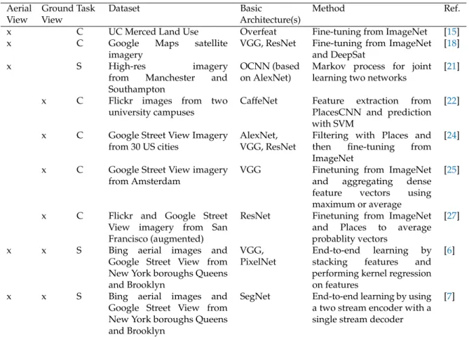
x C UC Merced Land Use Overfeat Fine-tuning from ImageNet [15]
x C Google Maps satellite
imagery
VGG, ResNet Fine-tuning from ImageNet and DeepSat
[18]
x S High-res imagery
from Manchester and Southampton
OCNN (based on AlexNet)
Markov process for joint learning two networks
[21]
x C Flickr images from two
university campuses
CaffeNet Feature extraction from PlacesCNN and prediction with SVM
[22]
x C Google Street View Imagery from 30 US cities
AlexNet, VGG, ResNet
Filtering with Places and then fine-tuning from ImageNet
[24]
x C Google Street View imagery from Amsterdam
VGG Finetuning from ImageNet
and aggregating dense feature vectors using maximum or average
[25]
x C Flickr and Google Street
View imagery from San Francisco (augmented)
ResNet Finetuning from ImageNet and Places to average probablity vectors
[27]
x x S Bing aerial images and
Google Street View from New York boroughs Queens and Brooklyn
VGG, PixelNet
End-to-end learning by stacking features and performing kernel regression on features
[6]
x x S Bing aerial images and
Google Street View from New York boroughs Queens and Brooklyn
SegNet End-to-end learning by using a two stream encoder with a single stream decoder
[7]
Table 1.Summary of different aspects of related work predicting land use with deep learning (C for a classification task, S for a segmentation task)
2.4.Aspects of the Machine Learning Problem of Urban Land Use
145
In contrast to many traditional remote sensing tasks, urban land use is highly complicated for a 146
number of reasons. First of all, the applications of urban land use are interested in land use classes 147
that are not measurable from space. Instead, they actually orient on the function of the building in the 148
complex ecosystem of the city. In addition, there are instances where buildings have changed their 149
function over time, for example, putting clubs or residential space into the manufacturing buildings 150
of industries that have left the city. In addition, it is not clear how land use can be structured into 151
a classification scheme at all. When defining classes from an application point of view, the classes 152
will not be well-defined and will have significant overlap. For example, many buildings mainly serve 153
residential purposes while still having shops and cafés inside. These issues need to be taken into 154
account when designing the classification scheme. 155
2.5. Contribution of This Paper
156
Urban building type mapping has not been addressing using both remote sensing and street view 157
images.This paper extends beyond state-of-the-art by exploiting two general aspects: first, the fact
158
that the information contained instreet viewimages and the information obtained from overhead
159
imagery are different and can be combined to improved performance, and second, the knowledgein 160
huge collections of images in the datasets Places365 and ImageNet in order to understand the image
161
content of both overhead imagery andstreet viewscenery.To achieve these goals, a comprehensive 162
comparison of existing models and fusion approaches was carried out. The contribution of this article 163
lies as follows. 164
• we compared two model fusion strategies: two-stream end-to-end fusion network (i.e. a
165
geometric-level model fusion), and decision-level model fusion. Deep networks applying on 166
individual data was also compared as baselines (i.e. no model fusion). A summary of the models 167
and fusion strategies exploited in this article, as well as the corresponding literature is shown in 168
Table2.
169
• we demonstrated that geometric combinations of the features of two types of images from distinct
170
perspectives, especially combining the features in an early stage of the convolutional layers, will
171
often lead to a destructive effect.
172
• without significantly altering the current network architecture, we propose to addressthis
173
problem through decision-level fusion of a diverse ensemble of models pre-trained from
174
convolutional neural networks. In this way, the significant differences in appearance of aerial and
175
street viewimages are taken into account in contrast to many multi-stream end-to-end fusion
176
approaches proposed in the literature.
177
• we have collected a diverse set of building images from 49 US states plus Washington D.C. and
178
Puerto Rico. Each building in this dataset consists of a set offourimages — one Google Street
179
View image, and three Google aerial/satellite images at an increasing zoom level.
180
3. Methodology
181
In order to find the best fusion strategy, we performed comparison of several state-of-the-art deep
182
neural networks, as well as different model fusion strategies. A summary of the CNNarchitectures 183
and fusion strategies exploited in this article, as well as the related literature can be seen in Table2.
184
3.1. The Datasets
185
In order to investigate fusion methods for building instance classification based on both remote
186
sensing andstreet viewimages, a corresponding benchmark datasetwas created for this paper. As
187
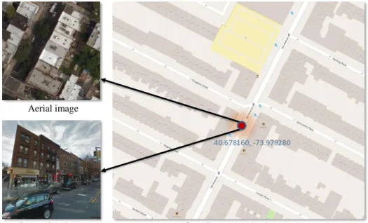
illustrated in Figure1, we extracted geolocation and the attributions of building function annotated
188
by volunteers from OSM. Then the associatedstreet viewimages and the overhead remote sensing
189
images of each building instance were retrieved via BingMap API and Google Street View API
190
using its geolocation [31]. We set our program so that the retrievedstreet viewimages point toward
191
the geolocation of each building. Three different zoom levels (17, 18, and 19 in the Google Maps
192
convention) of overhead remote sensing images approximately centered at the building’s geolocation
193
were downloaded. The finest zoom level19is approximately 30cm pixel spacing. The images cover 49
Basic
Architecture(s)
Method Section Related
Work
VGG, Inception Fine-tuning from ImageNet 3.2 [15,24]
VGG Fine-tuning two stream network from ImageNet by stacking convolution layer horizontally
3.3 [25,27] VGG Fine-tuning two stream network from ImageNet by
stacking dense layer vertically
3.3 [25,27] VGG, Inception Fine-tuning single stream from ImageNet and
Places365 then blend decision layers
3.4.1 [27] VGG, Inception Fine-tuning single stream from ImageNet and
Places365 then stack decision layers with additional machine learning algorithm
3.4.2
-Table 2.Summary of the CNN models and different fusion strategies exploited in this article.
OpenStreetMap database Aerial image
Street view image
Figure 1.A illustration of the creation of the dataset. For each building, we look for the nearest Google street view image that pointing toward it, and the aerial image patch that centered on it. The label of the building is extracted from the OSM building tag.
states (except Rhode Island) of the US, as well as Washington, DC and Puerto Rico, 51 areas in total.
195
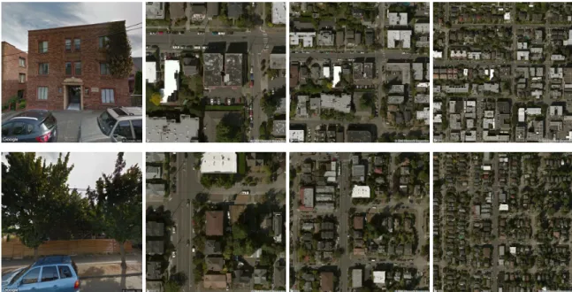
An example of our dataset can be seen in Figure2, where the images of two buildingsare displayed, 196
one building per row. Despite thestreet viewimages point to each building,there is often occlusion
197
due to existing vehicles and trees. This renders the fusion problem particularly challenging.
198
Given the issues of urban land use described in2.4, we follow a very basic but widely accepted
199
classification scheme with four classes: commercial,residential,public, andindustrial. To derive the
200
class of each building, we extracted them from the volunteered building tag from OSM. However, 201
as these tags are volunteered, their vocabulary can vary considerably, and even include spelling 202
errors. Therefore, we selected the 16 most frequently occurring building tags in our raw dataset and 203
aggregated them into four cluster classes:commercial,industrial,public, andresidential. Table3shows the
204
mapping and the number of buildings for each tag in detail. In summary, our dataset consists of 56,259 205
buildings with four images for each building. Among them, the images from the state of Wisconsin 206
and Wyoming were used as validation samples (1,943 buildings), those from the state of Washington 207
and West Virginia were used as test samples (2,212 buildings), and those from the remaining 47 areas 208
were used as training samples (52,104 buildings). 209
It is important to note that apart from the vocabulary difference and spelling error in the building 210
tag, OSM also faces ambiguities in their finer classification scheme that is defined in the OSM Wiki. For 211
Figure 2.Examples of Google Street View and the corresponding overhead remote sensing images with zoom levels19, 18, and 17in our dataset. Thestreet viewimage is pointing to the building instance. The remote sensing images are approximately centeredonthe building instance. As shown in the example on the second row, occlusion often happens in thestreet viewimages due to vehicles and trees. This renders the fusion problem particularly challenging.
many buildings it is simply not possible to assign a single class. Yet the OSM structure imposes the use 212
of a single tag for each building; hence, the volunteer’s choices significantly influence the consistency of 213
the building tags. These inaccuracies of the OSM label in the training data and the simplification of the 214
classification scheme are inevitable noise in the experiment set up. As a consequence, we cannot expect 215
classifiers with 99% accuracy as is sometimes reported for land use classification in different contexts. 216
Instead, a classification accuracy of about 60% to 80% on average would be a realistic expectation. 217
Cluster Class OpenStreetMap Tag # of Buildings
1 commercial commercial 5111 2 commercial office 3306 3 commercial retail 4906 4 industrial industrial 3839 5 industrial warehouse 2065 6 public church 4153 7 public college 1516 8 public hospital 1758 9 public hotel 2057 10 public public 1966 11 public school 4278 12 public university 4020 13 residential apartments 5039 14 residential dormitory 2154 15 residential house 5156 16 residential residential 4935
Table 3.Mapping of OpenStreetMap buildingtagsto general classes and instance numbers.
3.2. Fine-tuning Exisiting CNNs for Individual Image Types
218
To obtain a baseline performance, weapplied existingdeep neural networkspre-trainedon very
219
large datasets, including Places365 [32] and ImageNet [33], on our street view and aerial images,
220
respectively. These pre-trained models perform well for well-defined classification problems, where
VGG16 convolutional layers VGG16 convolutional layers 512 512 1024 256 256 256 4 (la bel) 64 conv1 fc1 fc3 fc2 fc4 VGG16 convolutional layers VGG16 convolutional layers 512 512 4096 8192 4 (la bel) fc1_1 fc1 pooling pooling 512 512 4096 4096 4096 fc2_1 fc1_2 fc2_2
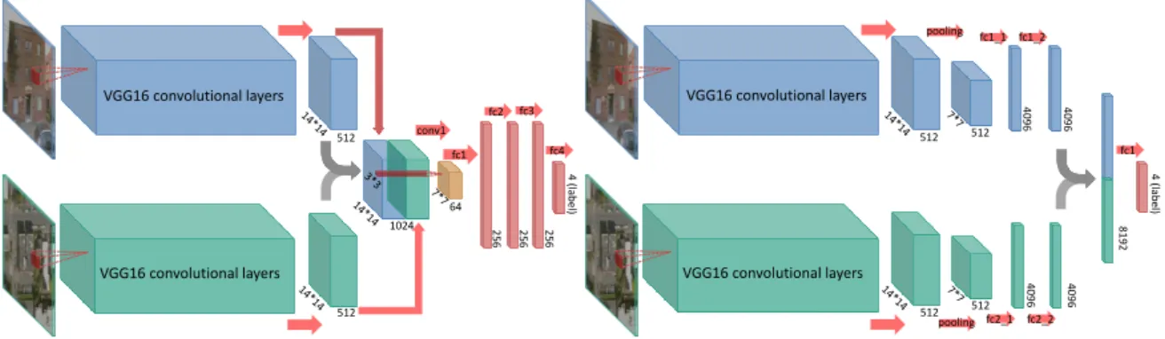
Figure 3.Thetwo two-stream fusion models used in the article. Themodel on theleft one concatenating the feature tensor (14*14*512) after the last convolutional layer of VGG16, and the right one concatenate the feature vector (4096*1) of the second last dense layer of VGG16. The fundamental difference is that the first model fuse the features earlier than the second model.
ImageNet is tailored to classes that refer to objects in images, while Places365 uses a classification
222
scheme that already classifies street view scenery. However, we have to adapt these models for our
223
classification schemeusingan iterated fine-tuningapproach, which is a standard approach in deep
224
learning. First, we remove the softmax layer from the pretrainedmodelsand train for a few epochs
225
with a new softmax layer fitting to the number of classes in our classification scheme. We apply a
226
constant dropout to this layer such that only parts of the connections are available during training, 227
while all connections will be used for inference. This technique is known to increase generalizability
228
by forcing the neurons toward learning things that are universally usefulrather thanuseful only
229
in relation to other neurons [34]. When this final new layer has converged a little bit, we iterate by
230
unlocking more layers and at the same time reducing the learning rate. In other words, we first train
231
the last layer, than the last few layers, and so on. Finally, we take averysmall learning rate and let the
232
training continue with all layers. In this way, the network can gradually adapt to our case without
233
destroying too much information in early layers due to fine-tuning with completely random final
234
layers.
235
3.3. Fine-tuning Two-Stream End-to-End Networks
236
The second method is two-stream end-to-end networks that is proposed in multiple literatures
237
for image fusion. We fine-tuned the existing CNN pre-trained on a large dataset for the two-stream
238
network,using an approachsimilar to the training strategydescribedin the previous section. We
239
selectedVGG16 pre-trained on ImageNet as our base network in this section, as it will bedemonstrated 240
in section4.1that different pre-trained networks provide comparable performance in the single-stream
241
case. For the input data, we useedthestreet view, and the aerial images with zoom level 19.
242
In the experiments, we fused the features ofstreet viewand remote sensing images in two slightly
243
different methods:inoneweconcatenatedthe bottleneck features (two 14*14*512 tensors) after the
244
last convolutional layer of VGG16, andinthe otherweconcatenatedthe features (two 4096*1 vectors)
245
at the secondtolast dense layer of VGG16. The architectures of the two fusion models can be seen
246
in Figure3. In the first fusion model, we appendeda convolutional layer with 64 filters, and 3 dense
247
layers of 256 nodes each after the concatenated feature tensor. In the second fusion model, we simply
248
concatenatedthe second to last dense layers of the two-stream VGG16, before the final dense layer.
249
Batch normalizationanddropout were also added after the concatenated features in both fusion
250
models. The structure of the first fusion model, including the number of convolutional and dense
251
layers, the number of filters in the convolutional layer, as well as the dropout rate, weredetermined 252
using Bayesian optimization [35].
253
The fine-tuning consistedof two stages thatweresimilar to the procedures described in the
254
previous section. First, we lock the convolutional layers of VGG16 and use Bayesian optimization to
Many probabilistic classifiers (e.g., VGG, ResNet, diverse parameter sets)
4
(lab
el)
Many probabilistic classifiers (e.g., VGG, ResNet, diverse parameter sets)
4 (lab el) Mean … 4 (lab el)
Many probabilistic classifiers (e.g., VGG, ResNet, diverse parameter sets)
4
(lab
el)
Many probabilistic classifiers (e.g., VGG, ResNet, diverse parameter sets)
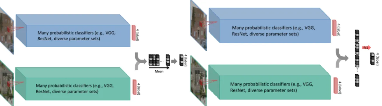
4 (lab el) fc1 … 4 (lab el)
Figure 4. A schematic drawing of the two decision-level fusion strategies — model blending (left) and model stacking (right) — exploited in this article. Model blending takes the mean of the softmax layer of multiple models, while model stacking concatenates those softmax vectors, and connects to a final softmax layer. Both of the fusion strategies act on a decision level, which allows networks for individual data type to be trained independently.
select a relatively good set of hyperparameters, such as learning rate and dropout rate, for training the
256
rest of the network. To reduce the computational effort, a maximum of 30 epochswas allowed for each
257
trial in the Bayesian optimization. After 100 trials, the best set of hyperparameters was used to train
258
the network for a dozen epochs,untilthere wasa little bit more convergence. As mentionedabove,
259
the architecture of the first fusion model was also jointly optimized in this process. Afterwards, we
260
progressively unlockedeach convolutional block of the two-stream VGG16 network in three steps, at
261
the same time reducing the learning rate by approximately one to two orders of magnitude.
262
3.4. Decision-level Model Fusion
263
Different from the two feature fusion strategies described in the previous section, decision-level 264
fusion combines the softmax probabilities or directly the classification labels. We exploited two 265
decision-level fusion strategies —model blending, andmodel stacking— in this section. The architectures
266
of the two fusion strategies are shown in Figure4, where model blending takes the mean of the
267
softmax layer of multiple models, while model stacking concatenate those softmax vectors. Both of the 268
fusion strategies act on a decision level, which allows networks for individual data type to be trained 269
independently. 270
3.4.1. Fusion through Model Blending
271
The first decision-level fusion approach considered in our work is known as model blending.
It is a very simple yet surprisingly powerful fusion scheme for probabilistic classifiers.In this case,
the probability vectors of many different models are being averaged in order to create the probability vector that is then finally used for classification. In this way, if one modality is very certain about a class and the other modality is less certain, the average tends to select the right class from the certain model. If, however, both models are uncertain, it is likely that the average represents this uncertainty as well. In addition, it is possible that biases average out. As an extreme example, consider a model
thatchoosesclass A out of {A,B} with a probability vector of {0.6,0.4} and a second model B that does
the opposite,i.e., chooses B with 0.6 and A with probability 0.4. Then the average model will choose A and B with 0.5probability. In this ideal example, two biased models have been blended and the bias is reduced. The downside of mean fusion is that it does not really allow for greedy strategies: it is not clear that a model that is not performing very well is not able to clarify errors of another well-performing model. Therefore, all combinations of models must be checked for an exponentially growing number of
n! k!(n−k)!
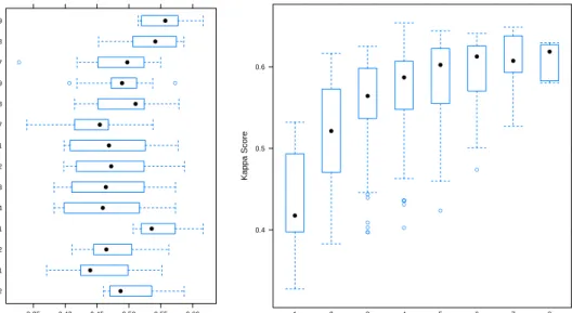
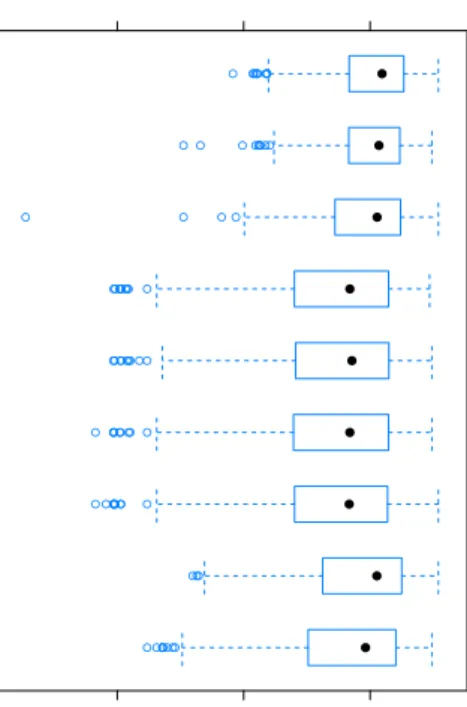
Kappa VGG16−Places365−Streetview−2 VGG16−Places365−Streetview−1 VGG16−ImageNet−Streetview−2 VGG16−ImageNet−Streetview−1 Inception3−ImageNet−Streetview−4 Inception3−ImageNet−Streetview−3 Inception3−ImageNet−Streetview−2 Inception3−ImageNet−Streetview−1 VGG16−ImageNet−A17 VGG16−ImageNet−A18 VGG16−ImageNet−A19 Inception3−ImageNet−A17 Inception3−ImageNet−A18 Inception3−ImageNet−A19 0.35 0.40 0.45 0.50 0.55 0.60 ● ● ● ● ● ● ● ● ● ● ● ● ● ● ● ● ●
(a) Statistics of the set of Kappa values for all models built by fusing the named model with another model
Number of Models Kappa Score 0.4 0.5 0.6 1 2 3 4 5 6 7 8 ● ● ● ● ● ● ● ● ● ● ● ● ● ● ● ● ● ● ● ● ●
(b) Performance relative to number of models
Figure 5.Performance of ensembles with up to two members and performance of ensembles of varying size.The figure depict a summary of the distribution of different ensembles formed with certain models inside or with certain numbers of models by indicating the distribution spread and mean.
possible fusion models withnas the number of baseline models andkas the maximum number of 272
models fused together. In order to deal with this situation, we first performedonly pair-fusion with all
273
our models and rejectedmodels inside each modality thatwere outperformed by other models in all
274
minimum, average, and maximum performance of any ensemble theywere inside.
275
3.4.2. Fusion through Model Stacking
276
Another approach to the combination of machine learning models is generally known asmodel
277
stacking and consists of using the individual models for feature extraction and then combining
278
the resulting concatenated features into a single feature vector per item. In our case, we took the
279
probabilistic vector output from each of the base models andconcatenate theminto a new vector —
280
one vector for each building in the test and validation sets. Then, wecouldtrain a simple classifier on
281
thisvector,mapping the probabilistic outputs to the classes.
282
4. Experiments and Discussion
283
4.1. Performance of Existing CNNs on Individual Data
284
We performed the fine-tuning protocol described in3.2with varying numbers of parameters and
285
base architectures on our datasets, and recorded the individual model performance given in Table4.
286
Without excessive tuning, we reachedperformances in the range of 57% precision (57% recall, F1 of
287
0.56) for one fine-tuned VGG-16 without global weight decay pretrained on Places365 to 68% precision
288
(66% recall, F1 of 0.66) for an Inception model pretrained on ImageNet fine-tuned with aerial imagery
289
of zoom level 19. The overall best model according to the Kappa score is a VGG-16 model pre-trained
290
on ImageNet and fine-tuned with street view imagery. From this table, wecanalready see that the best
291
two individual models are the best model from aerial and the best model from street view highlighting
292
that both modalities are powerful for themselves.
293
Table4listsonlya certain set ofrepresentativebase modelsfromseveral hundreds of models we
294
have trained. For example, VGG16-Places365-Streetview-1 and VGG16-Places365-Streetview-2 differ
Model Precision Recall F1-Score Kappa Inception3-ImageNet-A19 0.68 0.66 0.66 0.52 Inception3-ImageNet-A18 0.68 0.63 0.60 0.47 Inception3-ImageNet-A17 0.59 0.55 0.51 0.33 VGG16-ImageNet-A19 0.65 0.60 0.59 0.42 VGG16-ImageNet-A18 0.60 0.60 0.59 0.42 VGG16-ImageNet-A17 0.59 0.55 0.54 0.34 Inception3-ImageNet-Streetview-1 0.63 0.58 0.58 0.41 Inception3-ImageNet-Streetview-2 0.63 0.59 0.59 0.42 Inception3-ImageNet-Streetview-3 0.62 0.57 0.58 0.40 Inception3-ImageNet-Streetview-4 0.62 0.57 0.57 0.39 VGG16-ImageNet-Streetview-1 0.67 0.67 0.67 0.53 VGG16-ImageNet-Streetview-2 0.61 0.59 0.59 0.41 VGG16-Places365-Streetview-1 0.57 0.57 0.56 0.37 VGG16-Places365-Streetview-2 0.67 0.65 0.65 0.49
Table 4.Performance of individualclassifierswith varying modality and pre-training datasets.
Model Batch Dropout Decay N1 l1 N2 l2 N3 l3
Inception3-ImageNet-A19 32 0.2 - 10 0.0002 10 0.0002 10 0.0001 Inception3-ImageNet-A18 32 0.2 - 10 0.0002 10 0.0002 10 0.0001 Inception3-ImageNet-A17 32 0.2 - 10 0.0002 10 0.0002 10 0.0001 VGG16-ImageNet-A19 32 0.2 1e-05 10 0.0003 50 0.0003 - -VGG16-ImageNet-A18 32 0.2 1e-05 10 0.0003 50 0.0003 - -VGG16-ImageNet-A17 32 0.2 1e-05 10 0.0003 50 0.0003 - -Inception3-ImageNet-Streetview-1 64 0.2 - 10 0.0002 10 0.0002 10 0.0001 Inception3-ImageNet-Streetview-2 32 0.2 - 10 0.0001 10 0.0001 10 5e-05 Inception3-ImageNet-Streetview-3 64 0.3 - 10 0.0002 10 0.0001 50 5e-05 Inception3-ImageNet-Streetview-4 64 0.35 - 10 5e-05 10 0.0002 20 0.0001 VGG16-ImageNet-Streetview-1 64 0.2 - 10 0.0002 10 0.0002 20 0.0001 VGG16-ImageNet-Streetview-2 32 0.2 1e-04 10 0.0002 10 0.0002 10 0.0001 VGG16-Places365-Streetview-1 32 0.2 1e-04 10 0.0002 10 0.0002 10 0.0001 VGG16-Places365-Streetview-2 64 0.2 1e-04 5 0.0002 10 0.0001 20 0.0001
Table 5.Mostimportanttrainingparameters for the given models.
only in the batch size (32 and 64,respectively). Thegenerallearning parameters are given in Table5.
296
In this table,Batchrefers to the batch size used during stochastic gradient descent,Decayis the global
297
weight decay parameter added to the error function,andNiare the number of epochs that training is
298
performed with learning rateli. The difference between theNiis that we gradually unlock more layers
299
during fine-tuning.
300
In summary, we can conclude that individual modalities can be fine-tuned from pretrained
301
weights into a performance range of about 50%–70% in all precision, recall, and F1 score.
302
4.2. Performance of Two-stream End-to-End Networks
303
As mentioned in section3.3, the training of two-stream models consisted of two stages. The first
304
stage, we trained the networks with the convolutional layers of VGG locked; while in the second 305
stage we progressively unlocked the VGG convolutional layers in a way similar to that described in 306
section3.2.In the first stage of fine-tuning, the validation accuracy of both fusion models ranges from
307
40% to 60%. In the second stage, we attempted different combinations of decreasing learning rates, 308
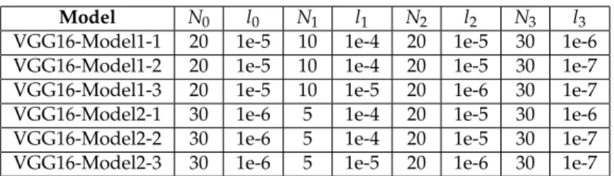
which areshownin Table6. In this table,N0andl0refer to the number of epochs and the learning
309
rate,respectively, of the best model in the Bayesian optimization step. N1,N2,N3andl1,l2,l3are the
310
settings for thethreesteps in the second stageoffine-tuning. In the second stage of the fine-tuning, we
311
found thatalearning rategreaterthan 1e-3 will not train the network at all. Therefore, we startedwith
312
alearning rate of 1e-4.
Model N0 l0 N1 l1 N2 l2 N3 l3 VGG16-Model1-1 20 1e-5 10 1e-4 20 1e-5 30 1e-6 VGG16-Model1-2 20 1e-5 10 1e-4 20 1e-5 30 1e-7 VGG16-Model1-3 20 1e-5 10 1e-5 20 1e-6 30 1e-7 VGG16-Model2-1 30 1e-6 5 1e-4 20 1e-5 30 1e-6 VGG16-Model2-2 30 1e-6 5 1e-4 20 1e-5 30 1e-7 VGG16-Model2-3 30 1e-6 5 1e-5 20 1e-6 30 1e-7
Table 6.The mostimportant training parameters for the two two-stream fusion models. N0andl0refer to the number of epochs and the learning rate of the best model in the Bayesian optimization step.N1, N2,N3andl1,l2,l3are the settings for the 3 steps in the second stage fine tuning, which are similar to those in Table5.
Model Precision Recall F1-Score Kappa
VGG16-Model1-1 0.63 0.62 0.62 0.50 VGG16-Model1-2 0.61 0.62 0.60 0.48 VGG16-Model1-3 0.66 0.61 0.61 0.47 VGG16-Model2-1 0.68 0.67 0.67 0.57 VGG16-Model2-2 0.66 0.67 0.66 0.55 VGG16-Model2-3 0.65 0.65 0.64 0.53
Table 7. The performance of the two fusion models w.r.t. different hyperparameters settings. The second fusion model in general outperforms the first one in general. Larger learning rate in the first step also helps to achieve better classification accuracy.
The performance of the fusion models evaluated on the test samples can be seen in Table7.It 314
is clear that, the second fusion model outperforms the first one in general. Thelarger learning rate
315
in the first step also helps to achieve better classification accuracy. However, compared to the model
316
trained from individual image types in section3.2, the two fusion models do not show significant
317
improvementinclassification accuracy. Despite the second fusion model slightly outperformingthe
318
best individual VGG model in Table4, the fusion often leads to a destructive effect. This is especially
319
true for the first fusion model. We believethisis due to the misalignment of the geometry of the
320
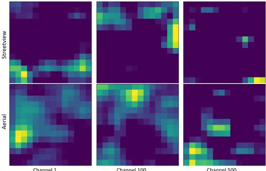
bottleneck features of the two image types. To illustrate this, an example of the bottleneck feature
321
tensors (14*14*512) of an image pair in our dataset is shown in Figure6, where the first, the 100th, and
322
the 500th channel of the tensor are plotted. As we can see the activated areas (in yellow and green)
323
of the feature maps of the two images are distinct. A geometric fusion of those two feature maps,
324
such as averaging or concatenation, will likely produceadestructive effect on the capability of pattern
325
recognition. In contrast, the features after the dense layers of VGG16 contain less geometric information
326
than the bottleneck features. Hence, better classification accuracy is achieved by fusing the feature
327
vector after the dense layers. If furtherinduction proceedsin a similar vein, it can be expected that the
328
best performance will be achieved by a decision-level fusion of the output softmax probabilities of the
329
two-stream network, which is basically training the two stream networks independently. Therefore,
330
we decided to use a decision-level fusion of the models trained from individual data sources.
331
4.3. Performance of Decision-level Fusion
332
4.3.1. Model Blending
333
Figure5(a)depicts the statistics of the performance of ensembles whichcontainthe specified
334
model and exactly one other model. It clearly shows that ensembles containing aerial views
335
fine-tuned from Inception outperform those fine-tuned using VGG16 architecture on average and
336
onquantiles. Therefore, we do not include the VGG16-based models for the aerial layers in the
337
final ensembling, expecting that their function is better fulfilled from Inception models for these
338
modalities. Similarly, we remove VGG16-ImageNet-Streetview-2,as it is significantly outperformed by
Str
ee
tvie
w
Aerial
Channel 1 Channel 100 Channel 500
Figure 6.Exampleof theVGG16bottleneck features ofthe street view(upper row) and the overhead remote sensing images (lower row) of one building in our dataset,which shows a probable reason of two-stream end-to-end fusion modelnotoutperforming simpler decision-level fusion models. The first, 100th, and 500th channels of the bottleneck feature (14*14*512 tensor) of one image pairs in our dataset are plotted. We can see that the geometry of the feature maps in general do not align, because a significant amount of spatial information is still contained in the bottleneck features. Such misalignment is common in most of the 512 bands as well as in most ofstreet viewand aerial image pairs. A geometric fusion, such as average or concatenate, will likely to produce destructive effect on the capability of pattern recognition.
VGG16-ImageNet-Streetview-1 and we remove VGG16-Places365-Streetview-1,as it is outperformed
340
by VGG16-Places365-Streetview-2 for the following complete subset fusion experiment on the
341
remaining 10 models.
342
For the remaining base models, we performed mean fusion and gave the best model results
343
depending on the number of models we fusedin Table8for up to four member models. Adding more
344
models did not improve performance. Figure5(a) Table8illustrates thatthe best model does contains
345
the two extreme zoom levels as well as two different architectures for street view classification. The
346
fusion process brings up the performance numbers from about 67% for the best individual model (cf.
347
Table4) to about 74% – 76% precision and recall.
348
We analyzedthe overall fusion approach and efficiency by looking into a selected set of base
349
models and all possible fusion combinations out of this. The number of base models in this casewas
350
quite limited, as the number of possible subsets grows with the factorial of the number of base models.
351
We then visualizedtwo aspects of the overall fusion. First, we plottedthe fusion model performance,
352
given the number of base models in the fused model. This is depicted in Figure5(b). The figure clearly
353
shows that the median performance, as given by the Kappa score,increases asthe number of base
354
modelsisadded to the ensemble. In addition, the variance of the performance tends to decrease with
355
the additional effect that the overall best model is not the model with the highest number of base
356
models. Instead, it is one of the models with many, yet not too many models. In other words,while it
357
is valid to expect the quality of models to increase by fusion, the largest model doesnotyieldthe best
358
performance. Instead, the model with four elementsdiscussed aboveis the overall best model from all
359
possible fusions of the selected set of ten base models.
360
Theusefulness of the various base modelswas analyzed.For each model, Figure7shows a plot of 361
the performance of all the blended models that contain the individual models listed in the figure.Note
# of Models Precision Recall F1-Score Kappa Models in Ensemble 2 0.74 0.73 0.73 0.62 Inception3-ImageNet-A19 VGG16-ImageNet-Streetview-1 3 0.74 0.74 0.73 0.63 Inception3-ImageNet-A18 VGG16-ImageNet-Streetview-1 Inception3-ImageNet-Streetview-2 4 0.76 0.76 0.75 0.65 Inception3-ImageNet-A19 Inception3-ImageNet-A17 VGG16-ImageNet-Streetview-1 Inception3-ImageNet-Streetview-4 Table 8. Performance of the best mean fusion models with varying number of member models. It illustrates that the best model does contains the two extreme zoom levels as well as two different architectures for street view classification. The fusion process brings up the performance numbers from about 67% for the best individual model (cf. Table 4) to about 74% – 76% precision and recall. Adding more models did not improve performance.
that in this case a large variance is actually a sign of a useful model: it has been used in bad models
363
as well, which might just contain fewer element models. What is interesting about this plot is that
364
our expectations can be clearly seen.For example, if the highly detailed zoom level 19 is part of an
365
ensemble, then the overall ensemble tends to be better than if itonlycontainsstreet viewmodels. This
366
fact can be derived, because the difference in distributions does stem from all models that contain one
367
but not the other as all models that contain both modalities come up in both distributions depicted in
368
the Figure. Consequently, we can see that street view has a significant contribution also independent
369
from fusing it with zoom level 19 aerial imagery.
370
4.3.2. Model Stacking
371
In the previous section, we showed that mean fusion is already able to bring the individual
372
multimodal models to a significantly improved fusion precision without investing any additional
373
information, such as another train-test split.In the model stacking fusion strategy, weused thetest set 374
for training and the validation set for finally evaluating.In general, we have seen that this does not
375
provide a significant improvement over the model blending from the previous section. We used logistic
376
regression (75.2% precision, 73.2% recall) , naive Bayes (72.9% precision, 71% recall), and Random
377
Forests (75.1% precision, 72.3% recall). As canbe seen, none of these models significantly outperforms
378
the mean fusion performance.
379
Given that models that contain both aerial and streetview modalities will contribute identically to 380
this figure, the variations come from models that use only one of the two mentioned modalities. In
381
conclusion, we can see that both modalities add independent value to the classification. Still, these
382
advanced stacking methods can be used to inject additional behavior into the classification thatcannot 383
be obtainedfrom the base models that are trained on accuracy and cross entropy loss. For example,
384
applying naive Bayes still leads to good values. What is particularly interesting is the fact that naive
385
Bayes can work with minorities very well. This leads to a model with 56% precision for the industrial
386
case, which is significantly higher than any of the other models. That is, for specific applications, the
387
framework of stacking can well be used to steer into cost-sensitive classifications concentrating on
388
certain classes. The results for this classifier (naive Bayes applied to the probabilistic output of all
389
models on the test set, numbers extracted from the validation set) are depicted in Figure8.
390
In our situation, we think that the number of instances is too small to train significant classifiers
391
on top of the output of the trained classifiers and that the effective reduction in available training
392
data implied by additional train-test splitting turns down the effectiveness of this approach. Still, for
393
significantly larger datasets, it is a promising direction because it can be more selective than model
394
averaging. In fact, this approach could base decisions on data-varying subsets of classifiers,while
Kappa VGG16−Places365−Streetview−2 VGG16−ImageNet−Streetview−1 Inception3−ImageNet−Streetview−4 Inception3−ImageNet−Streetview−3 Inception3−ImageNet−Streetview−2 Inception3−ImageNet−Streetview−1 Inception3−ImageNet−A17 Inception3−ImageNet−A18 Inception3−ImageNet−A19 0.4 0.5 0.6 ● ● ● ● ● ● ● ● ● ● ● ● ● ● ● ● ● ● ● ● ●●●●●●● ● ● ●●●●●● ● ● ● ●● ● ● ● ● ● ● ● ●●● ● ● ● ● ● ● ● ● ●● ● ●●●●●●● ● ● ● ● ● ● ● ● ● ●
Figure 7.Performance of fusion models containing a selected model.The figure depict a summary of the distribution of different ensembles formed with certain models inside or with certain numbers of models by indicating the distribution spread and mean. In the figure, our expectations can be clearly seen. For example, if the highly detailed zoom level 19 is part of an ensemble, then the overall ensemble tends to be better than if contains street view models. In general, the performance of different model ensembles are comparable. In conclusion, we can see that both image modalities add independent value to the classification.
the model blending case includes all classifiers into each decision. For our situation, this additional
396
capability did not pay off. Itis probablethat a larger test set would improve the ability of learning
397
in the stacking phase;however, it reduces the data for the individual model training. In essence, we
398
conclude that with the limited size datasets of remote sensing applications, mean fusion is the best
399
approachas it does not consume additional data for training a second level of classifiers.
400
4.3.3. Influence of the Zoom Level on Classification Behavior
401
It is difficult to assess the value of each model in fusion settings,as it is always to be seen relative
402
to the other models. If a model’s individual performance is low this does not mean that the model
403
does not pay off in fusion. It could be, for example, very strong on the cases that some combination of
404
other models is getting wrong and therebycould beadding a lot to the ensemble.
405
In order to still get some insight into the behavior of our classification problem with respect to
406
aerial zoom levels, we analyzedthe most simple models with different zoomlevelsin detail: We
407
combinedthe best fine-tunedstreet viewmodel with the best fine-tuned models for all selected zoom
408
levels. Performances for these models are given in Table9.
409
This table shows a clear trend for average performance: Higher-resolution imageryismore fruitful
410
in our setting,as opposed to lower resolution imagery. However, when digging into the actual model
411
details, we see another interesting aspect. For the industrial class, we get the following picture: the
412
maximal F1-score is attained for both models with zoom 19 and with zoom 17;models with zoom 17
413
show a higher precision of 64% as opposed to 59% for zoom level 19. This is most likely related to
414
the fact that some industrial buildings are very large and better represented in a lower zoom level.
415
Similarly, the highest recall for the residential class is achieved from low-resolution imagery as well, 416
Commercial Industrial Public Residential Commercial Industrial Public Residential 274 50 109 27 36 84 27 2 51 38 508 40 27 9 148 513 100 200 300 400 500
Figure 8.Performance ofnaive Bayesstacking for all models.This leads to a model with 56% precision for the industrial case, which is significantly higher than any of the other models. That is, for specific applications, the framework of stacking can well be used to steer into cost-sensitive classifications concentrating on certain classes.
Model Precision Recall F1 Kappa
Streetviewonly 0.67 0.67 0.67 0.53
Streetview-Aerial 17 0.70 0.69 0.68 0.55 Streetview-Aerial 18 0.73 0.71 0.70 0.57 Streetview-Aerial 19 0.74 0.73 0.73 0.62
Table 9. Performance of fusion best street view model with best aerial models. It shows that higher-resolution imagery is more fruitful than the lower resolution counterparts in our setting. Interestingly, for the industrial class (not shown in the table), models of zoom 17 outperforms the rest. This is most likely related to the fact that some industrial buildings are very large and better represented in a lower zoom level.
with 93%recall. However, the precision in this case is comparably low,only 67%. With increasing
417
resolution, the precision increases while the recall decreases (77% precision, 89% recall for zoom level
418
18; 84% precision with 80% recall for zoom level 19). In other words,when it comes to the classification
419
of many buildings, the context given by larger zoom levels turns out to be very useful while at the
420
same time increasingthe probability of missing out instances for a decreased recall.
421
These findings are supported by the fact that the best fusion model among the chosen four models
422
combinesstreet viewwith zoom 17 and zoom 19, with performances of 74% precision, 74% recall, and
423
73% F1. In this case, zoom 18 is most likely left out, because the information it can add is already part
424
of the models for the neighboring zoom levels. In fact, the model fusionwithall three zoom levels and
425
street view is outperformed by four models taking into account only one or two of the aerial models.
426
Finally, the performance of any of the aerial models is lower than the performance of anyfusion 427
modelsthat contain thestreet viewperspective, and the ensemble models that contains only the
428
street viewmodels. Thisindicatesthat thestreet viewperspective adds missing information to the
429
usual remote sensing perspective and that the results of this papercould not be achievedfrom aerial
430
observation only.
431
4.3.4. Best Model Discussion
432
Figure 9 depicts various confusion matrices for several best performing models. Several
433
differences between the modalitiesare readily apparent. For example, the beststreet viewmodel
434
depicted in Figure9(a)was able to correctly classify commercial buildingsforonly 64% of the cases,
435
while the best aerial model depicted in Figure9(b)reached77% of the cases. This might be related
436
to the fact that commercial buildings occur in patterns along major roads that are usually not visible
437
instreet view. To the contrary, public buildings are correctly classified in 66%of the caseforstreet
438
viewas opposed to 61% for aerial. Looking into the actual misclassification, we see that this difference
Commercial Industrial Public Residential Commercial Industrial Public Residential 295 31 95 39 49 51 36 13 107 18 423 89 38 11 109 539 100 200 300 400 500
(a) Best Streetview
Commercial Industrial Public Residential
Commercial Industrial Public Residential 355 26 37 42 87 32 22 8 175 8 388 66 71 3 113 510 100 200 300 400 500 (b) Best Aerial
Commercial Industrial Public Residential
Commercial Industrial Public Residential 342 13 62 43 76 42 22 9 66 5 479 87 18 2 62 615 150 300 450 600
(c) Best Fusion Model
Commercial Industrial Public Residential
Commercial Industrial Public Residential 340 15 64 41 77 47 17 8 86 9 474 68 24 2 63 608 150 300 450 600
(d) 2nd Best Fusion Model
Figure 9.Confusionmatrices for four selected models.The best street view model depicted in subfigure (a) was able to correctly classify commercial buildings for only 64% of the cases, while the best aerial model depicted in (b) reached 77% of the cases. This might be related to the fact that commercial buildings occur in patterns along major roads that are usually not visible in street view. To the contrary, public buildings are correctly classified in 66% of the case for street view as opposed to 61% for aerial. Looking into the actual misclassification, we see that this difference stems mainly from misclassifications into the commercial class. For the fusion models, we see that they outperform all single models in all four classes by a significant margin.
stems mainly from misclassifications into the commercial class. Thisis consistent withour intuition, as
440
the settling structures visible from above should be quite similar for commercial and public buildings
441
and their distinctions are easier froma street viewperspective.
442
For the fusion models, we see that they outperform all single models in all four classes by a
443
significant margin. It is interesting to observe,however,that the second-best fusion model is better
444
with respect to the industrial class while worse with respect to the distinction of public and commercial
445
classes. This is another hint that many of the top ensemble models can be relevant for application tasks
446
and realize several tradeoffs between classes.
447
5. Conclusions
448
This article comparedtwodifferent strategies — geometric feature fusion, and decision-level
449
fusion — for fusing ground-levelstreet viewimages and nadir-view remote sensing images with the
450
application of building functions classification. Our experiments conclude that without sophisticated
451
design of feature fusion mechanism in the network, a decision-level fusion ofstreet viewand overhead
452
images often outperforms a feature-level fusion, despite its simplicity. Our explanation is that the
453
misalignment of the geometry of features maps of the two image types will causeadestructive effect
when combining them purelygeometrically. This is especially true when combining the feature maps
455
in an early stage of the convolutional layers. Therefore, this argument is also generally applicable to
456
any images with distinct imaging perspective, geometry, or content, for example, radar and optical
457
images.
458
To this end, we employed decision-level fusion strategies to achieve great performance without
459
significantly alteringthe current network architecture. We let the individual networks for each image
460
type be trained independently, so that the significant differences in appearance of aerial andstreet 461
viewimages are taken into account,in contrast to many multi-stream end-to-end fusion approaches
462
proposed in the literature.Asignificant performance boost can be further achieved by usingamodel
463
ensemble, such as model blending and model stacking. Experiments showedthat model blending
464
without additional information, taking into account the uncertainty of the classifiers quantified in the
465
softmax probabilistic layer, brings a significant gain.This approach broughtclassification precision
466
from up to 68% for the best unimodal model to 76% for the best fusion model, taking into account
467
street viewand aerial imagery at the same time.
468
It is not surprising that the remote sensing images with the highest zoom level in general
469
give better performance than those with less zoom level, because of the higher spatial resolution.
470
However,inthe classification of residential areas, the image with the lowest zoom level outperforms
471
the high-resolution images. This is because the contextual information helps to better determine
472
residential buildings surrounded by similar ones. Therefore, our proposed method can be tailored to
473
different applications, by combining different image types, zoom levels, as well as different models.
474
Author Contributions:conceptualization, Xiao Xiang Zhu; methodology, Martin Werner, Eike Jens Hoffmann,
475
and Yuanyuan Wang; software, Martin Werner, Eike Jens Hoffmann, and Yuanyuan Wang; validation, Martin
476
Werner, Eike Jens Hoffmann,and Yuanyuan Wang; formal analysis, Martin Werner, Eike Jens Hoffmann,and
477
Yuanyuan Wang; investigation, Martin Werner, Eike Jens Hoffmann,and Yuanyuan Wang; data collection, Jian
478
Kang, Yuanyuan Wang; writing–original draft preparation, Eike Jens Hoffmann, Yuanyuan Wang, Martin
479
Werner; writing–review and editing, Martin Werner, Eike Jens Hoffmann, Yuanyuan Wang, and Xiao Xiang
480
Zhu; visualization, Martin Werner, Eike Jens Hoffmann, and Yuanyuan Wang; supervision, Xiao Xiang Zhu;
481
project administration, Xiao Xiang Zhu; funding acquisition, Xiao Xiang Zhu.
482
Funding:This work is supported by the European Research Council (ERC) under the European Union’s Horizon
483
2020 research and innovation programme (grant agreement number ERC-2016-StG-714087, Acronym: So2Sat,
484
www.so2sat.eu), and Helmholtz Association under the framework of the Young Investigators Group "SiPEO"
485
(VH-NG-1018, www.sipeo.bgu.tum.de).
486
Conflicts of Interest:The authors declare no conflict of interest. The funders had no role in the design of the
487
study; in the collection, analyses, or interpretation of data; in the writing of the manuscript, or in the decision to
488
publish the results.
489
Abbreviations
490
The following abbreviations are used in this manuscript:
491 492
CNN Convolutional Neural Network OSM OpenStreetMap
SVM Support Vector Machine CVUSA Cross-View USA dataset [8]
493
494
1. Koch, T.; Körner, M.; Fraundorfer, F. Automatic Alignment of Indoor and Outdoor Building Models
495
Using 3D Line Segments. 2016 IEEE Conference on Computer Vision and Pattern Recognition Workshops
496
(CVPRW), 2016, pp. 689–697. doi:10.1109/CVPRW.2016.91.
497
2. Rumpler, M.; Tscharf, A.; Mostegel, C.; Daftry, S.; Hoppe, C.; Prettenthaler, R.; Fraundorfer, F.; Mayer, G.;
498
Bischof, H. Evaluations on multi-scale camera networks for precise and geo-accurate reconstructions from
499
aerial and terrestrial images with user guidance.Computer Vision and Image Understanding2017,157, 255 –
500
273. doi:https://doi.org/10.1016/j.cviu.2016.04.008.
3. Bansal, M.; Sawhney, H.S.; Cheng, H.; Daniilidis, K. Geo-localization of street views with aerial image
502
databases. Proceedings of the 19th ACM international conference on Multimedia - MM ’11; ACM Press:
503
Scottsdale, Arizona, USA, 2011; p. 1125. doi:10.1145/2072298.2071954.
504
4. Majdik, A.L.; Albers-Schoenberg, Y.; Scaramuzza, D. MAV urban localization from Google street view
505
data. 2013 IEEE/RSJ International Conference on Intelligent Robots and Systems; IEEE: Tokyo, 2013; pp.
506
3979–3986. doi:10.1109/IROS.2013.6696925.
507
5. Zhai, M.; Bessinger, Z.; Workman, S.; Jacobs, N. Predicting Ground-Level Scene Layout from Aerial
508
Imagery. arXiv preprint arXiv:1612.027092016.
509
6. Workman, S.; Zhai, M.; Crandall, D.J.; Jacobs, N. A Unified Model for Near and Remote Sensing. IEEE
510
International Conference on Computer Vision (ICCV), 2017.
511
7. Cao, R.; Zhu, J.; Tu, W.; Li, Q.; Cao, J.; Liu, B.; Zhang, Q.; Qiu, G.; Cao, R.; Zhu, J.; Tu, W.; Li, Q.; Cao, J.;
512
Liu, B.; Zhang, Q.; Qiu, G. Integrating Aerial and Street View Images for Urban Land Use Classification.
513
Remote Sensing2018,10, 1553. doi:10.3390/rs10101553.
514
8. Workman, S.; Souvenir, R.; Jacobs, N. Wide-Area Image Geolocalization with Aerial Reference Imagery.
515
2015, pp. 1–9.
516
9. Hu, S.; Wang, L. Automated urban land-use classification with remote sensing. International Journal of
517
Remote Sensing2013,34, 790–803. doi:10.1080/01431161.2012.714510.
518
10. Ruiz Hernandez, I.E.; Shi, W. A Random Forests classification method for urban land-use mapping
519
integrating spatial metrics and texture analysis.International Journal of Remote Sensing2018,39, 1175–1198.
520
doi:10.1080/01431161.2017.1395968.
521
11. Zhu, X.X.; Tuia, D.; Mou, L.; Xia, G.S.; Zhang, L.; Xu, F.; Fraundorfer, F. Deep Learning in Remote Sensing: A
522
Comprehensive Review and List of Resources2017.5, 8–36,[1710.03959]. doi:10.1109/MGRS.2017.2762307.
523
12. Sermanet, P.; Eigen, D.; Zhang, X.; Mathieu, M.; Fergus, R.; LeCun, Y. OverFeat: Integrated Recognition,
524
Localization and Detection using Convolutional Networks2013. [1312.6229].
525
13. Russakovsky, O.; Deng, J.; Su, H.; Krause, J.; Satheesh, S.; Ma, S.; Huang, Z.; Karpathy, A.; Khosla, A.;
526
Bernstein, M.; Berg, A.C.; Fei-Fei, L. ImageNet Large Scale Visual Recognition Challenge. International
527
Journal of Computer Vision2015,115, 211–252. doi:10.1007/s11263-015-0816-y.
528
14. Yang, Y.; Newsam, S. Bag-of-visual-words and spatial extensions for land-use classification. Proceedings
529
of the 18th SIGSPATIAL International Conference on Advances in Geographic Information Systems - GIS
530
’10; ACM Press: New York, New York, USA, 2010; p. 270. doi:10.1145/1869790.1869829.
531
15. Marmanis, D.; Datcu, M.; Esch, T.; Stilla, U. Deep Learning Earth Observation Classification
532
Using ImageNet Pretrained Networks. IEEE Geoscience and Remote Sensing Letters2016, 13, 105–109.
533
doi:10.1109/LGRS.2015.2499239.
534
16. Simonyan, K.; Zisserman, A. Very Deep Convolutional Networks for Large-Scale Image Recognition2014.
535
[1409.1556].
536
17. He, K.; Zhang, X.; Ren, S.; Sun, J. Deep Residual Learning for Image Recognition. 2016 IEEE Conference
537
on Computer Vision and Pattern Recognition (CVPR). IEEE, 2016, pp. 770–778. doi:10.1109/CVPR.2016.90.
538
18. Albert, A.; Kaur, J.; Gonzalez, M.C. Using Convolutional Networks and Satellite Imagery to Identify
539
Patterns in Urban Environments at a Large Scale. Proceedings of the 23rd ACM SIGKDD International
540
Conference on Knowledge Discovery and Data Mining - KDD ’17; ACM Press: New York, New York, USA,
541
2017; pp. 1357–1366. doi:10.1145/3097983.3098070.
542
19. Basu, S.; Ganguly, S.; Mukhopadhyay, S.; DiBiano, R.; Karki, M.; Nemani, R. DeepSat. Proceedings of the
543
23rd SIGSPATIAL International Conference on Advances in Geographic Information Systems - GIS ’15;
544
ACM Press: New York, New York, USA, 2015; pp. 1–10. doi:10.1145/2820783.2820816.
545
20. Cheng, G.; Han, J.; Lu, X. Remote Sensing Image Scene Classification: Benchmark and State of the Art.
546
Proceedings of the IEEE2017,105, 1865–1883. doi:10.1109/JPROC.2017.2675998.
547
21. Zhang, C.; Sargent, I.; Pan, X.; Li, H.; Gardiner, A.; Hare, J.; Atkinson, P.M. An object-based convolutional
548
neural network (OCNN) for urban land use classification.Remote Sensing of Environment2018,216, 57–70.
549
doi:10.1016/J.RSE.2018.06.034.
550
22. Leung, D.; Newsam, S. Exploring Geotagged images for land-use classification. Proceedings of the ACM
551
multimedia 2012 workshop on Geotagging and its applications in multimedia - GeoMM ’12; ACM Press:
552
New York, New York, USA, 2012; p. 3. doi:10.1145/2390790.2390794.