How the Republic of Korea's financial structure affects the volatility of four asset prices

POLICY RESEARCH WORKING PAPER

2327

How the Republic of

structure affects the volatility

lKore,a

s

l'itiaLncial

Structure

Affects the

V l t

of F

l

Attec

atii1ty o

ts t ile AZoi

Fo;lr

u

Asset Prices

Hong G. Min Jong-goo Park

The World Bank

Development Data Group

Macroeconomic

Data Team

H

Public Disclosure Authorized

Public Disclosure Authorized

Public Disclosure Authorized

| POLICY RESEARCH WORKING PAPER 2327

Summary findings

Min and Park explore how Korea's financial structure others' diminish, suggesting that monetary policies

affects the volatility of asset prices. Documented should target different asset markets to achieve different

empirical evidence of the relationship between financial goals. If the goal of the monetary authority is to stabilize

structure and financial crisis sheds light on the the money market rate, for example, intervening in the

relationship between asset price volatility - extreme banking sector is more efficient than intervening in other

variations in prices - and financial structure. And the financial subsectors.

volatility of financial and nonfinancial asset prices * The higher volatility of stock prices reflects the thin

provides an indirect link between an economy's financial stock market in Korea.

structure and the likelihood of financial crisis. * The stability of the yield on government housing

Using time-series data and a set of indicators bonds reflects the Korean government's policy of

measuring financial structure, Min and Park examine stabilizing the nation's housing supply by isolating the

how Korea's financial structure affects the volatility of housing market from the impact of Korea's financial

the real effective exchange rate, the money market rate, structure.

government bond yields, and stock prices. They find: * Restrictions on foreigners' ownership cf domestic

* There is a stable long-term relationship between stock in Korea during the period analyzed, and the fact

financial structure and volatility in the real effective that most capital flows through commercial banks, affect

exchange rate, the money market rate, stock prices, and the exchange rate, which is determined (at least in the

the yield on government housing bonds. short run) by capital flows in the foreign exchange

l Financial structure affects asset price variables market.

asymmetrically. Some variables' volatility increases and

This paper - a product of the Macroeconomic Data Team, Development Data Group - is part of a larger effort in the

group to understand the financial structure of developing countries based on empirical data. Copies of the paper are

available free from the World Bank, 1818 H Street NW, Washington, DC 20433. Please contact Premi Rathaan-Raj, room

MC2-742, telephone 202-473-3705, fax 202-522-3645, email address [email protected]. Policy Research Working Papers are also posted on the Web at www.worldbank.org/research/workingpapers. The authors may be contacted at [email protected] or [email protected]. April 2000. (33 pages)

The Policy Research Working Paper Series disseminates the findings of work in progress to encourage the exchange of ideas about development issues. An objective of the series is to get the findings out quickly, even if the presentations are less than fully polished. The papers cany the names of the authors and should be cited accordingly. The findings, interpretations, and conclusions expressed in this paper are entirely those of the authors. They do not necessarily represent the view of the World Bank, its Executive Directo;-s, or the

How the Republic of Korea's Financial Sthuctu:re Affects the Volatility

of Four Asset Prices

Hong G. Min * and Jong-goo Park**

*Director of GPI, INC., Washington, D.C. ** World Bank, Washington, D.C.

This research began when the first author was an economist at the Development

Research Group, World Bank. We are grateful to Giovanni Majnoni, Judith McDonald, S.Kwack for their very helpful comments but all remaining errors are our own.

I. Introduction

The literature on currency crises has provided a nurmber of suggestions about the

possib:le influence of financial structure on tne volatility of asset prices and capital flows.

There is by now a documented empiricai evidence of the relationship between the

financial structure and financial crisis. While this inay provide some indirect insight

about the relationship between asset volatility - interpreted as extreme variations of

prices - and financial structure, a more direct analys:is seems to be missing. Although

finance theory tells us that the linkage between the financial structure of the economy and

the likelihood of financial crises is provided by the volatility of financial and

non-financial asset prices, this intermediate link is still somewhat unexplored. Stock prices

often cdouble or fall in half in a space of a few years, when there seems to be no concrete

reason why stock prices shouid have changed at all. Sometimes speculative prices

change dramatically in a matter of days or even hours. On 19 October 1987, the day of the worst crash in U.S. stock market history, the Dowv Jones Industrial Average lost 16

percent of its value in the space of three hours, from 1 .15 p.m. to 4.00 p.m. Analyses of

news service records show that during that intervel of time there was virtually no

econoimic news except for the news of the stock market drop itself. Such evidence

would seem to suggest that the source of market vo]atility is something loosely called

"market psychology,' the charnging public expectations, attitudes, and theories about the

market (Shiller, 1992').

In this paper, we examine how the financial structure of an economy, Korea,

affects the asset price volatility of several key financial variables using time-series data.

To measure empirically the financial structure of a counitry we employ the recently

(Demirguc-Kunt and Levine, 1999). In section II, we describe the development of Korea's financial

structure. In section HI, we investigate the statistical properties of each time series used

in this study and test for a stable long-run relationship among financial structure and

volatility of four financial variables in Korea using Johansen's conintegration technique.

In section IV, we investigate the dynamic impact of financial structure on the volatility of

four financial variables using the vector-autoregression model. Conclusions are

presented in section V.

II. The Development of Korea's Financial Structure

This section will investigate the changes in financial structure and the underlying

regulation, tax, and legal changes that caused them. The most important policy measure

of government-led economic development in Korea was financial policy (e.g.,

interest-rate regulation and policy loans). The heavy intervention of the Korean government in

the financial system during the 1960s and 1970s is revealed by its discretionary allocation

of funds to target industries through policy loans (credit rationing). This caused

misallocation (overinvestment) of financial resources into the heavy manufacturing anid

chemical industries, which led to creditor bankers' losses. The banking sector suffered

from a lack of competitiveness, an accumulation of non-performing assets, and delays in

liberalization. Policy loans at preferential interest rates accounted for half of the total

credit offered by domestic financial institutions in 1970s and about 30 percent in the

1980s with the expansion of non-bank financial Institutions (NBFIs, hereafter; Bank of

Korea, 1995).

believing that a massive misallocation of resources in the heavy manufacturing and

chemical industriezs could have been avoided if the functioning of the financial system

had been left in the hands of the private sector. The government tried to improve

efficiency through the promotion of competition and private initiative. The goals of

financial reform were reducing inefficiency and preventing private rent-seeking and

foreign control of the financial market (Amsden and Euh, 1993).

1. Changes in Finaancial Structure, Size, Activity and Efficiency in Korea

Among financial institutions, banks provide fiunds mostly through loans and they

dominated in financial institution borrowings until the 1970s. Their relative importance

has gradually declined, slipping from 29.2 percent of the market in the first half of the

1970s to 19.2 percent in the first half of the 1990s, Whereas Table 1 shows that the

market shares of non-banks and securities market inzreased over the period 1970-74 to

1990-94 frorn 8.8 percent to 33.2 percent and from 1.1.1 percent to 27.0 percent

respectively. The share of deposits held by nonbanks increased from 31.6 percent in

1980 ito 67.6 percent in 1995 (see Table 2).

Despite the slow pace of reform, Korea's financial market experienced growth in

overall size and activity. Korean financial depth increased from 49.4 percent in 1981 to

103.2 percent in 1989 and to 150.0 percent in 1995, mostly due to the growth in the

nonbanking sector. However, stock market capitaliZation to GDP grew even more over

this period, from 65 percent to 63.4 percent. This explains the growth in the stock market's

relative size, which started out at 20 percent in early 1980s, but ended the decade at 90

percent. During the same period, stock market liquidity and bank credit to the private

percent of GDP. However, the growth in stock market liquidity far outweighed that in

bank credit as can be seen from relative activity figures. Looking at efficiency indicators,

relative efficiency increased whereas overall efficiency fell during the period. This is

because although stock market turnover increased with liberalization, banking spreads

increased even more.

2. Development of Non-Bank Financial Institutions

In this section, we will analyze the development of non-bank financial institutions

(NBFIs), their special treatment by law and regulation, their structure and business

activities, their role in stimulating and mobilizing savings, and their contribution to

Korea's economic development

Many NBFIs were introduced in 1972 in response to the Presidential Emergency

Decree for Economic Stabilization and Growth. Their numbers and volume of funds

grew significantly during the rapid economic growth of the 1970s and 1980s. A further

contribution to their rapid growth came from the relatively higher interest rates permitted

to them and the greater degree of autonomy in management they were allowed compared

to traditional banks. In 1982, requirements for establishing NBFIs were reduced and

consequently twelve short-tern finance companies and 57 mutual savings and finance

companies began operations. During the period 1987 to 1990, five securities trust

companies and eighteen life insurance companies were in operation (Bank of Korea,

1995).

NBFIs can be classified into four categories according to their business activities:

i) development institutions, which consist of the Korea Development Bank, the

Export-Import Bank of Korea, and the Korea Long Term Credit Bank; ii) investment instituticns,

securities investment trust companies; iii) savings institutions including trust accounts of

banks, mutual savings and finance companies, credit unions, mutual credit facilities,

community credit cooperatives, and postal savings; and iv) life insurance institutions.

Out of these four categories of NBFIs, investment and life insurance institutions grew

most rapidly during the period 1980-1995. These NBIFIs have contributed significantly

to the stimulation and mobilization of savings since they were able to circumvent the

interest-rate ceilings on both the sources and uses of iunds (Koo, 1993). Table 2 shows

that over the period 1]980-1995, the share of loans made by NBFIs increased from 36.7

percent to 57. 1] percernt. On the demand side, high real interest rates (due to slowing price

increases in the early 1980s) jeopardized the viability of firms with high financial

leverage. Because of the repressed commercial bark interest rates, corporations not

suppoited by the government were forced to borrow from NBFIs. NBFIs evaded the low

interest-rate policy of Ministry of Finance (MOF) by requiring compensating balances

that borrowers had to redeposit in the same financial institution, thereby raising the

effective interest rates on the original loans (Bank of Korea, 1995).

3. A Measure of Financial Structure

The measurement of financial structure in this study draws heavily on the recent

work by Demirguc-Kunt and Levine (1999) that derived several findings on the

relationship between financial structure and per capita income level. According to their

study, in higher income countries, banks and other financial intermediaries as well as

stock markets and the overall financial system tend to be larger, more active, and more

efficient. In higher income countries insurance companies, pension funds, and other

For practical purposes, we used three variables as indicators of Korea's financial

structure: bank assets to GDP (claims on the private sector by commercial banks to GDP,

BANK); non-banking financial institution's assets to GDP as a measurement of other

financial institution's size (NBFI); and stock-market capitalization to GDP as a measure

of stock market development (MK). Variable definitions are given in the Appendix.

Figure 1 shows the changing pattern of the financial structure in Korea and Figure 2

shows the volatility of four financial variables.

III. The Data and Their Statistical Properties

In this section we define the variables used in this study and test the stationarity of

those variables using two different unit root test procedures.

1. The Data and Their Statistical Properties

All quarterly data are from the March 1999 issue of the IMF's International

Financial Statistics, CD-Rom version, and are seasonally adjusted using exponential

smoothing. Data definitions are found in the Appendix. A control variable is used to

isolate the effects of structural variables (that are expected to maintain their impact over

the long run) from the short-run effects of policy -- monetary or fiscal -- on the volatility

of each economic variable a la Krumm (1993). Volatility responds to both real anid

monetary variables. Monetary and fiscal variables are combined into one

macroeconomic control variable, VV, which is defined as the percentage change in

domestic credit over and above the percentage change in GDP, foreign prices, and t]he

nominal exchange rate.

where DC is domestic credit, Y is GDP, Pf is U.S. WPI, NE; is the nominal exchange rate

to the U.S. dollar, and * indicates percentage change.

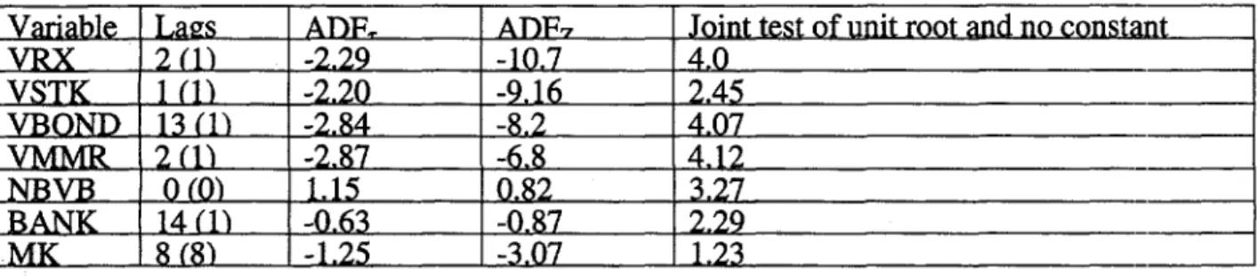
In order to examine the stationarity of each time series, we conducted unit root

tests. Table 3 reports the results from the Augmented Dic]key-Fuller and Paco Goerlich

Tests, which reveal that all series have unit roots.

2. Johansen's Coireation Test

Since all variables are non-stationary, we use Johansen's co-integration analysis to

test whether those variables have co-integrating vectors. Johansen (1988) and Johansen

and Juselius (1990) cleveloped a cointegration test methodology that overcome most of

the problems of the previous two-step approach.

Johansen and Juselius (1990) considered the following general model:

Xt = IIXtt- +...+Ht-Ik Xt-k +V+Et fort=l,....T, (2)

where X t is a vector of variables ; £, I... E T are independent and normal errors with zero mean and covarianct matrix 1; X t-k, X o are fixed; and v is an intercept vector. Economic timne series are often non-stationary and systenms such as the above

vector-autoregressive representation (VAR) can be written in the conventional first-difference

form:

AXt = Fki AX t-k-1 + I Xt-k + V + £t (3)

where r i = l -- - -I rI F 2- ...lk) - for i=1,'2 ... k- 1,

and I = IH-k).

-- rI ...

-The orly level term in equation (3) is FIX t-k. Thus, only the Fl matrix contains

information about the long-run relationship between the variables in the data vector.

1. If the rI matrix has rank zero then all variables in X are integrated of order one or

higher and the VAR has no long-run properties;

2. If the Fl matrix has rank p (i.e., it is of full rank ), the variables in X are stationary; and

3. If rI matrix has rank r ( 0 < r < p), El can be decomposed into two distinct (p*r)

matrices a and

13

The third case implies that there are r cointegrating vectors. The parameters of

the cointegrating vectors are contained in the ,B matrix. Therefore 1'X is stationary even

though Xt itself is nonstationary. The a matrix gives weights with which the

cointegrating vectors enter each equation of the system. To determine the number of

cointegrating vectors, r, Johansen and Juselius (1990) used two likelihood-ratio tests.

The first test is based on the maximal eigenvalue (XMAX) -- the null hypothesis is that

there are at most r cointegrating vectors against the alternative r+l cointegrating vectors.

The second test is based on the trace of the stochastic matrix (TRACE) -- the null

hypothesis is that there are at most r cointegrating vectors against the alternative

hypothesis that there are r or more cointegrating vectors. Two likelihood-ratio tests for

the existence and cointegrating vectors are reported in Table 5. Johansen's cointegralion

tests are implemented using four lags and for four sets of five variables which include the

volatility, financial structure, and control variables.

Table 5-A shows that the volatility of stock prices has two cointegrating vecitors

with the financial structural variables at the 10 percent critical level based on both Xinax

and Trace statistics. One of the cointegrating vectors can be written as follows:

Equation (6) implies that increases in bank assets to GDP and stock market capitalization

to GDP increases the volatility of the stock price. This finding is consistent with the

impulse response analysis of the vector-autoregression model. The economic implication

of this cointegrating vector is that increase in bank assets (BANK) and stock market

capitalization (MK) destabilize the volatility of stock prices, implying a high sensitivity

of stock prices to financial activities of the economy. The impulse response function in

Figure 3 confirms this finding.

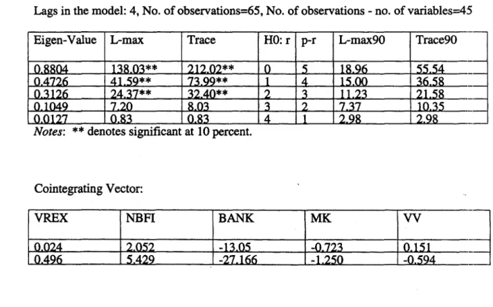
Table 5-B shows that the volatility of the real effective exchange rate has three

cointegrating vectors with the financial structure variables at the 10 percent critical level

based on both Xmax and Trace statistics. One of the cointegrating vector scan be written

as follows:

.024 VREX + 2052 NBFI - 13.05 BANK -.723 MK + 0.151 VV = 0 (7).

This cointegrating vector is consistent with the impulse response analysis of the

vector-autoregression model presented in Figures 4-A and 4-B.

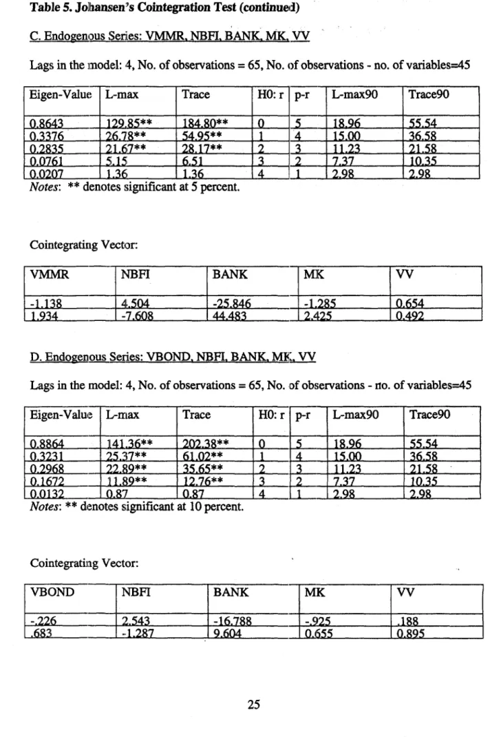
Tabl]e 5-C shows that the volatility of money-market interest rates has three

cointegrating vectors with the financial structural variables at the 10 percent critical level

based on both %ima;x and Trace statistics. One of the cointegrating vectors can be written

as follows:

-1.138 VMMR + 4.504 NBFI - 25.846 BANK-1.285 MK + 0.654 VV =0. (8) This implies that increases in non-bank financial institutions' assets to GDP increase the

volatility of the bond yield, whereas increases in stock market capitalization to GDP

decrease the volatility of money-market rates. This finding is consistent with the impulse

response analysis of the vector-autoregression model shown in Figures 5-A and 5-C. The economic implication of this cointegrating vector is that increases in stock market

capitalization to GDP and non-bank financial institutions' assets destabilize the volatility

of the money-market rate because their activities are less regulated than other financial

sector.

Table 5-D shows that the volatility of government bond yield has two

cointegrating vectors with the financial structural variables at the 10 percent critical level

based on both Xmax and Trace statistics. One of the cointegrating vectors can be written

as follows:

-.226 VBOND + 2.543 NBFI - 16.78 BANK -.925 MK + 0.188 VV = 0. (8)

This implies that increases in bank assets to GDP and stock market capitalization to GDP

decrease the volatility of the government bond yield. This finding is consistent with the

impulse response analysis of the vector-autoregression model which is presented in

Figure 6. The economic implication of this cointegrating vector is that while increases in

bank asset and stock market capitalization stabilize the volatility of the government bond

yield, increases in non-bank financial institutions' assets destabilize the volatility of the

government bond yields because their activities are less regulated.

IV. Dynamic Analysis Using a Vector-Autoregression Model

In this section we use the vector-autoregression model to examine the dynamic

impact of financial structure on the volatility of the financial variables.

1. A Vector-Autoregression Model

We will test the dynamic impact of changing financial structure on the volatility of four

economic variables using the vector-autoregressive model presented in equations (9)

through (13):

MK = I VRX + £oci BANK + £oq NBFI + Y.i VV (10)

BANK= axj MK + YX. VRX + Ic4 NBFI + X.0% VV (11)

NBFI = od MK + £ou BANK + Icx VRX + £ou, VV (12)

WV= £oci MK + £ocu BANK + £cx NBF1 + Ea %. VRX, (13)

where VRX is the volatility of the real effective exchange rate, MK is the amount of

stock market capitalization divided by GDP, BANKC is claims on the private sector by

commercial banks, NBFI is the ratio of bank to non-bank financial institutions' assets,

and W is the macroeconomic policy stance variable to control for the impact of

macroeconojmic policies.

2. Impulse Response Function

The goal of this section is to investigate the dynamic impact of financial

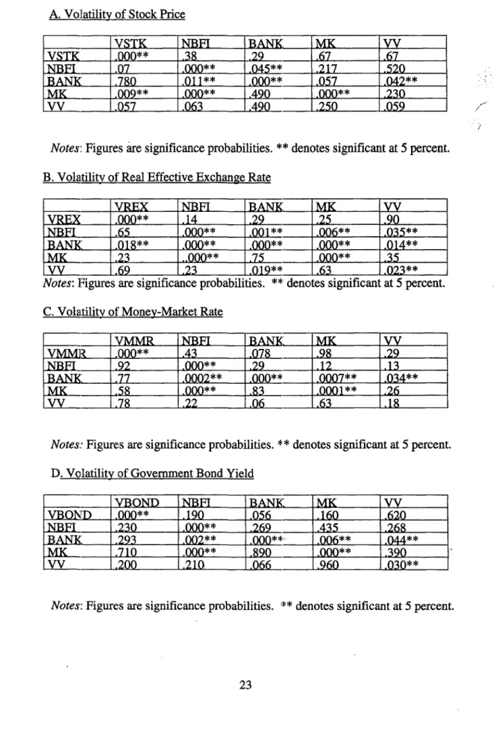
structural variables on the volatility of economic variab]Les. Granger-causality amongst

these variables is examined and the results are reported in Table 4. Based on these

causality tests and economic theory, the ordering of the variables in the

vector-autoregression is determined. Various different orderings are tried to see the robustness

of the test result.

The dynamic impact of financial structure and macroeconomic policy stance

variables are analyzed through the computation of variance decompositions (VDCs) and

impulse response functions (IRFs) which, in turn, are based on the moving-average

representation of the VAR model and reflect bcth direct and indirect effects. In

particular, the VDCs for VREX indicate the percenlage of the forecast-error variance in

3. Dynamic Impact of Financial Structure on Economic Volatility

An optimal lag of four is chosen based on the likelihood-ratio test and the model is then estimated. Since different orderings of the variables in the VAR estimation yield

different results, various orderings based on the Granger-causality tests reported in Table

4 were tried. However, different orderings did not bring about significant differences. From the impulse response function and variance decomposition of forecast-error variances, we find the following:

Volatility of the stock price

hnpulse response functions show that stock market capitalization (MK) and private claims of commercial banks (BANK) increase the volatility of the stock prices in Korea. Increased stock market capitalization increases the uncertainty of the market and leads to the increased volatility of stock prices -- this reflects the highly volatile characteristics of the stock price independent of the financial structure. Finally, the macroeconomic policy stance variable has a negative impact on VSTK The impulse response functions are shown in Figures 3-A to 3-C.

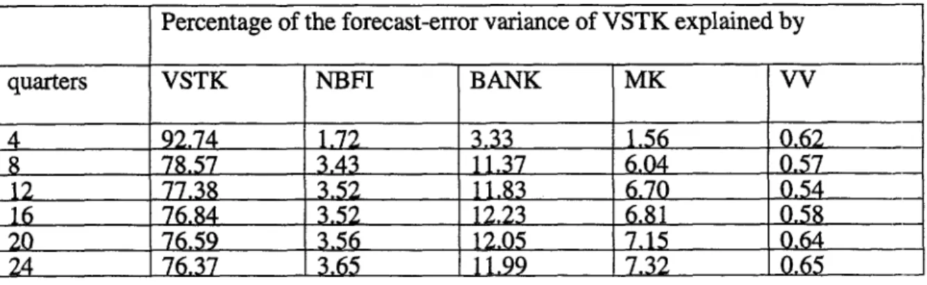
Table 6-A shows the innovation accountings of the volatility of the stock price. With the exception the stock price volatility variable itself, BANK plays the mnost

important role in explaining the variance decomposition of the forecast error variance of the volatility of the stock price, explaining about 12.percent of the 12-step ahead forecast error variance. The stock market capitalization to GDP (MK) variable is next in importance. However, the policy stance (VV) and stock market capitalization (MIK)

price volatility. I'able 6-C shows the variance decompiosition of the volatility of the

stock price from one to 48 quarters.

Volatility of real effective exchange rate

The impulse response function shows thal. stock market capitalization (MK)

increases the volatility of the real effective exchange rate, whereas private claims of

commercial banks to GDP (BANK) destabilize the volatility in Korea. This can be

explained by the strong restrictions on the foreigners'investments in Korea's stock market

and on most capital flows, which are one of the most important variables affecting

exchange-rate movements. Impulse response functions are shown in Figures 4-A to 4-C.

In sum, wit;h the exception of the real effective exchange rate itself, stock market

capitalization to GIDP plays the most important role in explaining the forecast error

variance of the volatility of the real effective exchange rate, explaining about 12 percent

of the forecast error variance by 8 quarters. The next most important explanatory

variable is private claims of the banking sector (BANK), explaining about 7 percent by 8

quarters. IHowever, the policy stance and non-bank financial institutions (NBFI)

variables explaini very little of the forecast-error variance of the volatility of the real

effective exchange rate. Table 6-B shows the varianrce decomposition of the volatility of

the real effective exchange rate in Korea.

Volatility of the money market rate (VMMR)

inpulse response functions are shown in Figures 5-A to 5-C. These indicate that

rate, while private claims of commercial banks (BANK) decrease the volatility of the

money-market rate. This implies that as a country moves from a bank-based financial

structure to a market-based financial structure, the volatility of the money-market rate

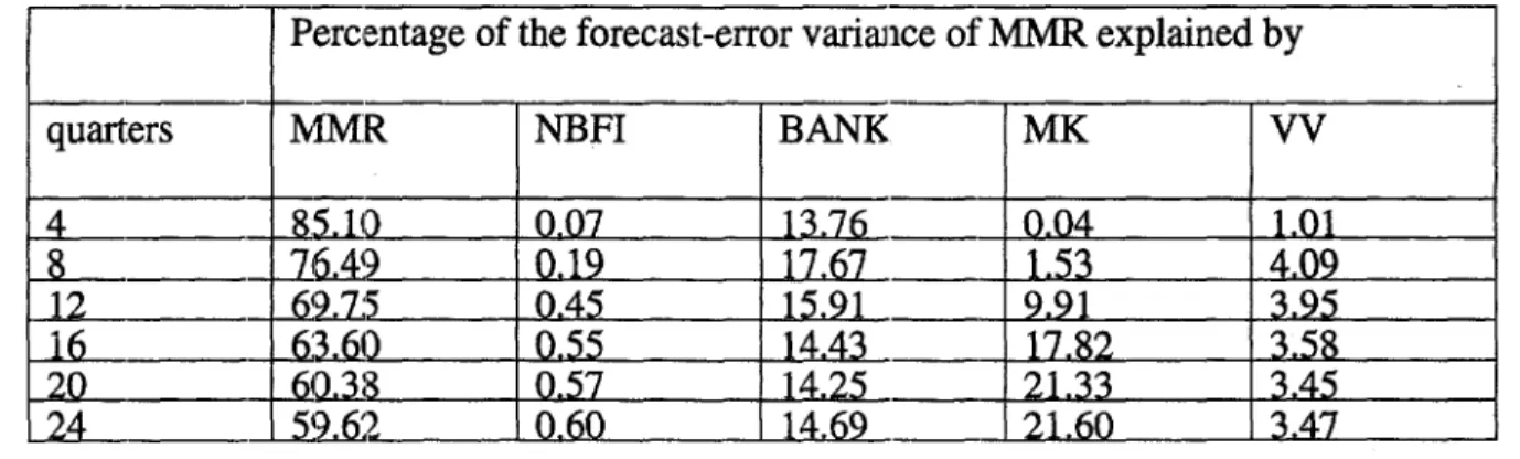
increases. From the variance decomposition of the forecast error variance of the

volatility of the money-market rate, except volatility of the money market rate itself,

stock market capitalization is playing the most important role, explaining some 22

percent of the forecast error variance in 24 quarters ahead (commercial banks claims on

private sector to GDP (BANK) is the next most important variable). Both the policy

stance variable (VV) and NBFI have very small roles to play in explaining the

forecast-error variance of the volatility of the stock price volatility. Table 6-C shows the variance

decomposition of the volatility of the money-market rate from one to 24 quarters.

Volatility of the Government Bond Yield on Housing

Both the stock market capitalization to GDP (MK) and private claims of

commercial bank to GDP (BANK) decrease the volatility of the government bond yield

on housing. This can be explained by the strong commitment of the Korean government

to supplying stable funds for new housing construction. However, an increase in the

macroeconomic policy stance variable (VV) causes an increase in the volatility of t]he

government bond yield. This finding is consistent with economic theory. The impulse

response function of BOND is shown in Figures 6-A, to 6-C.

When we move to the relative importance of financial structure on the

forecasting-error variance of the bond yield volatility, claims of the commercial bank: to

to GDP (MK) is plays the next most important role. Innovation accounting of the

government bond yield on housing is given in Table 6-D.

V. Conclusionis

This study tried to identify the role of financial structure on the volatility of

economic variables, the real effective exchange rate, the money-market rate, government

bond yield, and stock price. We used the concept of market-based and bank-based

financial structure developed by Demirguc-Kunt and Levine (1999) to investigate the

changing role of financial structure on the volatility of the economic variables. From

this case study of Korea, it is difficult to say that our findings are unique. However, some

of our more interesting findings, at least for Korea, are summrarized in what follows.

It seerns that there exist more than one long-run stable relationship between

financial structure and economic variables which are volatility of real effective exchange

rate, money market rate, stock price, and government boncl yields on housing in Korea.

We also found that the dynamic impact of financial structure on the volatility of each

economic variable is asymmetric, i.e., some economnic variable's volatility increased

whereas other variable's volatility decreased. For the stock price volatility, increased

claims to private sector by commercial bank to GDP and stock market capitalization to

GDP both increase the volatility of the stock price. This reflects the highly volatile

nature of stock prices, which is independent of Korea's financial structure.

For the volatility of the real effective exchange rate, claims to private sector by

commercial bank to GDP (BANK) increases volatilii:y and government should monitor

closely the comrnercial bank's activity in foreign exchange market to avoid their

capitalization to GDP (MK) decreases the volatility of the real effective exchange rates implying that as Korea's financial structure moves from a bank-based to a market-based system, the volatility of the real effective exchange rate decreased since mid-1980s even with a more flexible exchange rate system and this is confirmed by Figure 2.

Since the exchange rate is determined (at least in the short run) by capital inflows and outflows in the foreign-exchange market, this finding reflects the restrictions on foreigners' ownership of domestic stock in Korea during the analysis period and the iact that most of the capital flows are channeled through commercial banks.

For the volatility of the money-market interest rate, stock market capitalization to

GDP (MK) increases the volatility whereas increased claims to the private sector of commercial banks to GDP (BANK) decreases the volatility of the money-market rate. This implies that if interest targeting is the primary goal of policy authority, strong supervision and monitoring is necessary in the stock market to stabilize the money-market rate. For the volatility of the government bond yield, both the claims to private sector by commercial bank to GDP (BANK) and stock market capitalization to GDP (MK) decrease the volatility of the yield on government bond on housing. This explains

the intrinsic stability of the yield on govermment bond yield on housing. The Korean

government's policy goal of stabilizing the house supply in Korea has successfllly isolated the housing market from the impact of financial structure.

This study identified a stable long-run relation ship between financial structure and volatility of each financial variable in Korea, implying that stabilization policy should be different depending on priority of the policy goals. Future study will investigate whether the findings of this study are robust with respect to different definitions of financial structure and for different data sets, i.e., cross-country data.

References

Ahmed, B Ickes, P. Wang, and B.S. Yoo, 1993,"International Business Cycle," American

Economic Review, 83, 335-59.

Amsden, A.H. anid Y.D. Euh,1993, "South Korea's 1980s Financial Reforms: Good Bye Financial lRepression (Maybe), Hello New Institutional Restraints," World Development, 21, 379-390.

Bank of Korea, 1990, 1995, The Financial System in Korea, Seoul, Korea.

Cho, Y.J. and J.K. Kim, 1995, "Credit Policies and the Industrialization of Korea," World

Bank Discussion Paper No. 286, The World Bank, Washington D.C.

Demirguc-Kunt, A. and R. Levine, 1999, "Bank-based and Market-based Financial Systems: Cross-Country Comparisons," mimeo, The World Bank.

Demirguc-Kunt, A. and V. Maksimovic, 1996a, "Financial Markets and Firn Debt Maturity," World Bank Working Paper No. 1686, The World Bank.

, 1996b,

"Financial

Johansen, Soren, 1988, "Statistical Analysis of Cointegrating Vectors," Journal of

Dynamics and Control, 231-254.

Johansen, S. and K. Juselius, 1990, "Maximum Likelihood Estimation and Inference on Cointegralion -- With Application to the Demand ifor Money," Oxford Bulletin of

Economics and Statistics, May, 169-2 10.

Jung, J. and J1W. Lee, 1993, "Recent Financial Reforms in Korea: Real Name Financial System Launched," Korean Financial Review, vol. 3, no. 3, 3-22.

Kang, M.S., 1990, "Money Market and Monetary Policy in Korea," Korea Development Institute, Seoul, Korea.

Koo, B.H., 1993, "Industrial Policy and Financial Refoims in Korea," in Financial Sector

Reforms in Asia and Latin American Countries,, edited by Shakil Faruqi, The World

Bank.

Krumm, K.L., 1993, "A Medium-term Frameworl: for Analyzing the Real Exchange Rate with Applications to the Philippines and Tanzania," World Bank Economic Review, vol 2, May, 219-245.

Park, J.H., 1993, "Financial liberalization and Internationalization in Korea," Korean Financial Review, vol. 3, no. 4, 3-23.

Data Appendix: Sources and Definitions

1. RX: real effective exchange rate of Korean won from J]P Morgan.

2. BOND: government bond yield on housing (IFS line 61).

3. STK: stock price index (IFS line 62).

4. MMR: money-market rate (IFS line 60b).

5. VRX: volatility of real effective exchange rate defined as a six-month window standard deviation for each quarter; data are from JP' Morgan.

6. VBOND: volatility of the government bond yield on housing defined as a six-month window standard deviation for each quarter (IFS line 61).

7. VSTK: volatility of the stock price defined as a six-month window standard deviation for each quarter (IFS line 62).

8. VMMR: volatility of the money-market rate defined as a six-month window standard deviation for each quarter (IFS line 60b).

9. NBFI: Olher financial institutions' domestic assets (IFS lines 42a-d) to GDP (IFS line 9O bp).

10. iBANK: Commercial banks' domestic assets (IFS lines 22 a-d) to GDP (IFS line 90 bp).

11. MK: Stock market capitalization (Monthly Bulletin of the Stock Market) to GDP (IFS line 90 bp).

Table 1. Financial Market Composition of Korea* 1970-74 1975-79 1980-84 1985-89 1990-94 (1)Financial 38.0 40.7 45.6 48.7 52.5

Institutions

Notes: * denotes the non-financial sector's fund raising

CP denotes commercial paper

Table 2. IMarket Share of Financial Institulions iin Korea

Loans (in percent) Deposits (in percent)

1980

11985 11990

1995* 1980 11985

1990

1995*

Dep. Money Bank** 63.3 58.4 48.3 42.9 68.4 53.5 41.0 32.4

-32.2% -52.6% BIs*** 36.7 41.6 51.7 57.1 31.6 '146.5 59.0 67.6 55.6% 113.9% A.Development 14.8 10.8

18.3

4.1

9.0

11.1

Notes: 1)* dlenotes the amount by the end of June, 1995

2)** denotes money deposits at banks

3)**:1 denotes Non-banking Financial Institutions

4)% denotes the total growth rate between June 1980 and June 1995

Table 3. Tests of Unit Roots

A. Augmented Dickey-Fuller Test

Variable La2s ADF& ADF7 Joint test of unit root and no constant VRX 2 (1) -2.29 -10.7 4.0 VSTK I (1) -2.20 -9.16 2.45 VBOND 13 (1) -2.84 -8.2 4.07 VMMR 2 (1L -2.87 -6.8 4.12 NBVB O(0) 1.15 0.82 3.27 BANK 141 -0.63 -0.87 2.29 _ MK 1 (8) -1.25 -3.07 1.23

Note: ** denotes that the estimate is significant at 5 percent critical level.

B. Paco Goerlich Test

Variable AR r... t T-i Constant No constant, Conclusion

VRX 4 -1.29 -1.07 -1.12 Unit root. no drift VSTK 4 -1.61 -1.73 -0.75 Unit root. no drift VBOND 4 -2.90 -2.54 -1.09 Unit root. no drift VMMR 4 -2.50 2.3 .70 Unit root. no drifti-NBVB 4 -2.66 -0.12 N.A. Unit root. drift BANK 4 -1.79 -1.03 1.61 Unit root. no drift NK 4 -A1.98 2.19 1.29 Unit root no drift

Table 4. Gianger-Causality Test

A. Volatilitv of Stock Price

V VSTK NBFI BANK. MK yy VST .00o0±** .38 .29 .67 .67 NBFI _ .07 0 .000** .04**_ .217 .520 BAN .7.011 ** 000* .057 .042** MK _ .009** .000**_ 490 _ VV YŽLfi_- .057 .063

9

Notes: Figures are significance probabilities. ** denotes significant at 5 percent.

B. Volatility of Real Effective Exchange Rate

_I_REX NBFI I

BA

VREX=_ 000** .14 .29 .25 .90

NBFI __65 .000** .

_

BANK: .018 .

.000**

LMK__ . 3 .. 00* .. .357 .0**

WY _-69 .23 .019** 13023**

Notes: Figures are significance probabilities. ** denotes significant at 5 percent.

C._Volatility of Money-Market Rate

I_- 2 MMRt NBEI. NANNBFI MK Wy

Im VM00]* :, .43 .08 _ .98 .29

NBI _921 .00.2_.-.12 .13

BANK 77 ..0002*_. .0007** .034**

MK

_

W _- 78 .22 .06.63 .18

Notes.- Figures are significance probabilities. ** denotes significant at 5 percent.

D. Volatili:of Government Bond Yield

_ VBOND NBFI BANK MK yV

VBO[D .000** .190 .06 .160 620

NBFI ___230 .000** .269 _ 435 .268

BANK; _ .293 .002** .. 006** .044**

MK _- 710 .000** .80 .000** .390.

W _- .200 .210 _.066 1_960 .030**

Table 5. Johansen's Cointegration Test

A. Endogenous Series: VSTP. NBFI, BANK, MK. W

Lags in the model: 4, No. of observations=65, No. of observations - no. of variables=45

Eigen-Value L-max Trace HO: r p-r L-max90 Trace9O

0.8912 144.19** 208.74** 0 5 18.965

0.491l9 44.01 ** 64.55** 1 4 15.00 36.58 _ 0.2106 15.37** 20.54 2 3 11.23215 _ 0.0750 5.07 5.16 3 2 7.37 10.35 _

0.0014 0.09 0.09 4 1 2.98 2.98 _

Notes: ** denotes significant at 10 percent.

Cointegrating Vector:

VSTP NBFI BANK MK VW

-.058 -1.644 12.225 0.662 0.018

-0.7 6 = -2.739 0 19.046 _0.789 0.089_

B. Endogenous Series: VREX. NBFI. BANK. MK. W

Lags in the model: 4, No. of observations=65, No. of observations - no. of variables=45

Eigen-Value L-max Trace HO: r p-r L-max90 Trace90

0.884 138-03** 212.02** 0 5 18.96 5

0.47 6 41.59** 73.99** 1 4 15.00 3. _

0.3126 24.37** 32.40** 2 3 1.3 21.58 _ 0.1049 7.20 8.03 3 2 7.37 10.35 _

0.0127 0.83 0.83 4 1 2.98 2.98 _

Notes: ** denotes significant at 10 percent.

Cointegrating Vector:

VREX NBFI BANK MK _7

0.024 2.052 -13.05 -0.723 0.151

Table 5. JoRhansen's Cointegration Test (continued)

C. Endogenous Series: VMMR. NBFI. BANK MK. W

Lags in the model: 4, No. of observations = 65, No. of observations - no. of variables=45

Eigen-Value L-max Trace HO: r p-r L-max9O Trace90

0.8643 - 12&,85** 184.80** O 5 _18.96 ..- 55.54 0.3376 _ i8* 54.95** 1 4 _15.00 36.58 0.2835 _j1 28.17** 2 3._ 11.23 21.8 0.0761 _il6.51 3 2 _7,37 10.35 0.0207 _ 1-3 1.36 I 2.98 2.98

Notes: ** denotes significant at 5 percent.

Cointegrating Vector:

VMMR NBFI | BANK K VV

-1.138 4,k.504 -25.846 L285 0.654 1.934 -7.68 44.483 _ .L50.492

D. Endogenous Series: VBOND. NBFI. BANK MK. W

Lags in the model: 4, No. of observations = 65, No. of observations - no. of variables=45

Eigen-Value L-mrax Trace HO: r p-r L-max90 Trace9O

0.8864 - LLA1.36** 202.38** O 5 _18.96 55.54-0,323 1 -2537** 61.2* 1 4 _15.00 36.58 -0.629682_ _L;9* 35.65** 2 3W_11.23 21.58 0.1672 - 'L.9** -12.7-6** 3 2 _7.37 J0.35

0.0132 - (L_7 0.87 4 1 2.98 2.98

Notes: ** denotes significant at 10 percent.

Cointegrating Vector:

VBOND NBFI BANK MK W

-.226 _ _,.543 -16.788 _- '925 .188 .683 _ - 1.287 9.604 -0-655 02895

Table 6: Variance Decomposition of the VAR Model:

A. Decomposition of Volatility of Stock Price (VSTK)

Percentage of the forecast-error variance of VSTK explained by

quarters VSTK NBFI BANK MK VV

4 92.74 1.72 3.33 1.56 0.62_ 8 78.57L 3.43 11.37 6.04 0.57 1 2 7738 3.52 11.83 6.70 0.54_ 1 6 76.84 3.52 12.23 6.81 0.58 _ 20 76.59 3.56 12.05 7.15 0.64_ 24 76.37 3.65 11.99 7.32 0.65_

B. Decomposition of Volatility of Real Effective Exchange Rate (VREX)

Percentage of the forecast-error variance of VREX explained by

quarters VREX NBFI BANK MK VV

4 90.05 0.08 2.73 6.21 0.92 _ 8 80.23 _ 0.29 6.80 _ 11.57 108 _ 12 79.81 0.30 6.56 11.91 1.40 _ 16 7961 0.32 6.60 11.98 1.48_ 20 79.24 0.35 6.72 12.19 1.48 _ 24 7916 0.36 6.71 L 1227 1.48 _

Table 6: Vairiarnce Decomposition of the VAR Model (continued)

C. Decopsition of Volatility of Money-Market Rate (MMR)

Percentage of the forecast-error variance of' MMR explained by

quarters MMR NBFI BANK MK VV

4 8_ 1il) 0.07 13.76 _ 0.04 1.01 8 __ AL 0.19 17.67 _-1.53 4.09 12 6 9'5 0Q45 _ 15.91 _ 9.91 3.95 16 __ - 6: 0.55 14.43 17.82 3.58 .20 _60,3 3 0.57 1.5 _21.33 3.45 24 59_ 2 0.60 _ 2760 34_

D. Decomnposition of Volatility of Government Bond Yield (BOND)

Percentage of the forecast-error variar.ce of BOND explained by

quarters BOND NBFI BANK MK VW

4 __4 0.45 14.31 0.79 2.39 8 __L84 0.94 20.39 6.52 3.28 126 _ - 4 _ 10.7 22.26 6.96_ 16 64Li 1.10 22.21 9.09 3.12 20QI 61.01 1.04 20.97 14.01 2.95 24 - 10_ 1.04 2039 _ 17.67 2.82

Figure 1. Financial

Structure

of

Korea

3

-o

-.-

a

-

_

\BOND

STOCK

1973:01 1978:03 1984:01 1989:03 1995:01

Time

Figure 2. Volatility of Financial

Variables

40

40

3 0

___

VSTK

I

D)

20

|

020

-.--

VMMR

(UlO

- l.-

V

_VREXI

Figure 3. Cumulative Impulse Response Functions of Stock Price Volatility

A. Shock of Non-Bank Assets

Cumulative Impulse Response of

VSTK to NBFI

Quarters

B. Shock of Market Capitalization (MK)

Cumulative

Impulse Response of VSTK to

MK 6 4 2 0 1 3 5 7 9 11 13 15 17 19 21 23 Quarters

C. Shock of Bank Assets

Cumulative Impulse Response of VSTK to

BANK

10

1 3 5 7 9 11 13 15 17 19 21 23

Figure 4. Cumulative Impulse Response Functions, of REER Volatility

A. Shocks to Non-Bank Financial Institutions'Assets

Cumuilative

Impulse Response of VREX to

NBFI

0.2

0

-0.2

-04

Quarters

B. Shocks of Market Capitalizations

C:umulative

Impulse

Respons;e

of

VREX to MK

0

-1

-2

Quarters

C. Shocks of Bank Assets

Cumtuladtive

Impulse Response of VREX to

BANK

2

1

3

5

7

9 11 13 15 17 19 21 23

Quarters

Figure 5. Cumulative Impulse Response Functions of Money-Market Rate (MMR)

A. Shock of Non-Bank Assets

Cumulative Impulse Response of VMMR to NBFI 0.15 0.1 0.05 0 -0.05 Quarters

I.

B. Shock of Market Capitalization (MK

[

MK 1.5 1 0.5 0 | 1 3 5 7 9 11 13 15 17 19 21 23 Quarters

C. Shock of Bark Assets

Cumulative Impulse Response of

VMMR to BANK

0

-0.5 -1

Figure 6. Cumulatitve Impulse Response Functions; of Bond Yield Volatility A. Shocks of Non-Bank Financial Institutions' Assets

Cumullative Impulse Response of VBOND to

NBFI

B. Shocks oiF Market Capitalizations

Cumulative Impulse Response of VBIOND to

MK 0.5 0 -0.5 -1 Quarters

C. Shocks of Bank Assets

Cumulative Impulse Response of

VMMR

to

BANK

-05

Policy Research Woaking Paper Series

Contact

Title Author Date for paper

WPS2302 Why Liberalization Alone Has Not Klaus Deiningar March 2000 M. Fernandez

Improved Agricultural Productivity Pedro Olinto 33766

in Zambia.: The Role of Asset Ownership and Working Capital

Constrain-its

WPS2303 Malaria aid Growth F. Desmond McCarthy March 2000 H. Sladovich

Holger Wolf 37698

Yi Wu

WPS2304 Disinflaticin and the Supply Side Pierre-Richard Ag6nor March 2000 T. Loftus

Lodovico Pizzati 36317

WPS2305 The Impact of Banking Crises on Maria Soledad Martinez March 2000 A. Yaptemco

Money Demand and Price Stability Peria 31823

WPS2306 Internaticonal Contagion: Implications Roberto Chang March 2000 E. Mekhova

For Policy Giovanni Majnoni 85984

WPS2307 Surveying Surveys and Questioning Francesca Racanatini March 2000 P. Sintim-Aboagye

Questions: Learning from World Bank Scott J. Wallsten 37644

Experience Lixin Colin Xu

WPS2308 How Smail Should an Economy's Paul Beckerman March 2000 H. Vargas

Fiscal Deficit Be? A Monetary 38546

Programmincl Approach

WPS2309 What Drives Private Saving around Norman Loayza March 2000 E. Khine

the World? Klaus Schmicit-Hebbel 37471

Luis Serven

WPS2310 Hov. Politics and Institutions Affect Mitchell A. O0enstein March 2000 M. Leenaerts

Persion Reform in Three 84264

Postcommunist Countries

WPS2311 The Bueenos Aires Water Concession Lorena Alca2ar April 2000 P. Sintim-Aboagye

Manuel A. Abdala 38526

Mary M. Shirley

WPS2312 Measuring Governance, Corruption, Joel S. Hellman April 2000 D. Bouvet

anc State Capture: How Firms and Geraint Jones 35818

Bureaucrats Shape the Business Daniel Kaufrriann Environrieni in Transition Economies Mark Schankerman

WPS2313 Howv interesI Rates Changed under Patrick Honchan April 2000 A. Yaptenco

Financiai Liberalization: A Cross- 31823

Policy Research Working Paper Series

Contact

Title Author Date for paper

WPS2314 Technological Leadership and Beata K. Smarzynska April 2000 L. Tabada

Foreign Investors' Choice of 36896

Entry Mode

WPS2315 Investment in Natural Gas Pipelines Alejandro Jadresic April 2000 M. Salehi

in the Southern Cone of Latin America 37157

WPS2316 Distrubutional Outcomes of a Emanuela Galasso April 2000 P. Sader

Decentralized Welfare Program Martin Ravallion 33902

WPS2317 Trade Negotiations in the Presence of Keiko Kubota April 2000 L. Tabada

Network Externalities 36896

WPS2318 Regulatory Reform, Competition, Mark A. Dutz April 2000 H. Sladovich

and Innovation: A Case Study of the Aydin Hayri 37698

Mexican Road Freign Industry Pablo Ibarra

WPS2319 Externalities and Production Gunnar S. Eskeland April 2000 H. Sladovich

Efficiency 37698

WPS2320 Does More Intense Competition Lead Mark A. Dutz April 2000 H. Sladovich

to Higher Growth? Aydin Hayri 37698

WPS2321 Algorithms for Purchasing AIDS David Bishai April 2000 P. Sader

Vaccines Maria K. Lin 33902

C. W. B. Kiyonga

WPS2322 Self-Targeted Subsidies: The Richard H. Adams, Jr. April 2000 M. Coleridge-Taylor

Distributional Impact of the Egyptian 33704

Food Subsidy System

WPS2323 Globalization and Firms' Financing Sergio Schmukler April 2000 E. Khine

Choices: Evidence from Emerging Esteban Vesperoni 37471

Economies

WPS2324 Give Growth and Macroeconomic Brian Pinto April 2000 H. Makarenko

Stability in Russia a Chance: Harden Vladimir Drebentsov 87832 Budgets by Eliminating Nonpayments Alexander Morozov

WPS2325 Banking Systems Around the Globe: James R. Barth April 2000 A. Yaptenco

Do Regulation and Ownership Affect Gerard Caprio, Jr. 31823

Performance and Stability? Ross Levine

WPS2326 How Urban Concentration Affects Vernon Henderson April 2000 R. Yazigi