Optimal Sticky Prices under Rational Inattention

SFB 649 Discussion Paper 2005-040

Optimal Sticky Prices

under Rational

Inattention

Bartosz Ma

ć

kowiak*

Mirko Wiederholt*

* Humboldt-Universität zu Berlin, Germany

This research was supported by the Deutsche

Forschungsgemeinschaft through the SFB 649 "Economic Risk". http://sfb649.wiwi.hu-berlin.de

ISSN 1860-5664

SFB 649, Humboldt-Universität zu Berlin Spandauer Straße 1, D-10178 Berlin

S

FB

6

4

9

E

C

O

N

O

M

I

C

R

I

S

K

B

E

R

L

I

N

Optimal Sticky Prices under Rational Inattention

∗

Bartosz Ma´ckowiak

Humboldt University Berlin

Mirko Wiederholt

Humboldt University Berlin

First draft: June 2004. This draft: July 2005.

Abstract

In the data, individual prices change frequently and by large amounts. In standard sticky price models, frequent and large price changes imply a fast response of the aggre-gate price level to nominal shocks. This paper presents a model in which price setting

firms optimally decide what to observe, subject to a constraint on information flow. When idiosyncratic conditions are more variable or more important than aggregate conditions,firms pay more attention to idiosyncratic conditions than to aggregate con-ditions. When we calibrate the model to match the large average absolute size of price changes observed in the data, prices react fast and by large amounts to idiosyncratic shocks, but prices react only slowly and by small amounts to nominal shocks. Nominal shocks have persistent real effects. We use the model to investigate how the optimal allocation of attention and the dynamics of prices depend on thefirms’ environment.

JEL: E3, E5, D8.

Key words and phrases: rational inattention, sticky prices, real effects of nominal shocks.

∗_{We thank for helpful comments Klaus Adam, Michael Burda, Giancarlo Corsetti, Wouter DenHaan,}

Andrea Gerali, Federico Ravenna, Frank Smets, Harald Uhlig, David Vestin and seminar participants at Bocconi, Central European University, Columbia, Ente Einaudi Rome, European Central Bank, European University Institute, Goethe University Frankfurt, Humboldt University Berlin, IHS Vienna, London Busi-ness School, New York Fed, Princeton and SED 2005. Bartosz Ma´ckowiak thanks Chris Sims for conver-sations about rational inattention. Mirko Wiederholt thanks Ente Einaudi for hospitality. This research was supported by the Deutsche Forschungsgemeinschaft through the Collaborative Research Center 649

“An optimizing trader will process those prices of most importance to his de-cision problem most frequently and carefully, those of less importance less so, and most prices not at all. Of the many sources of risk of importance to him, the business cycle and aggregate behavior generally is, for most agents, of no special importance, and there is no reason for traders to specialize their own information systems for diagnosing general movements correctly.” (Lucas, 1977, p. 21)

1

Introduction

In the data, individual prices change frequently and by large amounts. Bils and Klenow (2004) and Klenow and Kryvtsov (2004) study micro data on consumer prices that the U.S. Bureau of Labor Statistics collects to compute the consumer price index. Bils and Klenow find that half of all non-housing consumer prices last less than 4.3 months. Klenow and Kryvtsov find that, conditional on the occurrence of a price change, the average absolute size of the price change is over 13 percent.1

At the same time, the aggregate price level responds slowly to monetary policy shocks. A variety of different schemes for identifying monetary policy shocks yield this result (e.g. Christiano, Eichenbaum and Evans (1999), Leeper, Sims and Zha (1996) and Uhlig (2005)). Uhlig (2005) finds that only about 25 percent of the long-run response of the U.S. GDP price deflator to a monetary policy shock occurs within thefirst year after the shock.

This combination of empirical observations is difficult to explain with standard models of sticky prices. The popular time-dependent model of price setting due to Calvo (1983) can explain a slow response of the aggregate price level to a monetary shock if: (a) firms in the model adjust prices infrequently;2 or (b) firms in the model adjust prices by small 1_{Thefinding that individual prices change frequently and by large amounts is robust to whether temporary}

price changes reflecting sales are included or not. When Bils and Klenow (2004) net out the impact of sales, the median price duration rises from 4.3 to 5.5 months. When Klenow and Kryvtsov (2004) net out the impact of sales, the average absolute size of price changes falls from 13.3 to 8.5 percent.

2

Galí and Gertler (1999) estimate the Calvo model using quarterly aggregate U.S. data. The estimated model implies that a typicalfirm waits about 5-6 quarters before changing its price.

amounts.3 However, neither (a) nor (b) seems to be true in the data.

Golosov and Lucas (2005) conduct numerical experiments with a state-dependent model of price setting. They use the micro data on consumer prices compiled and described by Klenow and Kryvtsov (2004) to calibrate a menu cost model with monetary shocks and idiosyncratic productivity shocks. In the calibrated model, the aggregate price level responds quickly to a monetary shock. The reason is that a firm setting a new price in a menu cost model takes into account current values of all shocks. Hence, frequent price adjustment implies a fast response of prices to all shocks, including monetary shocks.

This paper presents a model that can explain why individual prices change frequently and by large amounts and, at the same time, the aggregate price level responds slowly to monetary policy shocks. We study price setting by firms under “rational inattention” in the sense of Sims (2003). Firms can change prices every period at no cost. The profi t-maximizing price depends on the aggregate price level, real aggregate demand and an idio-syncratic state variable (reflecting consumers’ preferences or thefirm’s technology). Firms decide what to observe. Firms choose the number of signals that they receive every period as well as the stochastic properties of these signals. Firms face the constraint that the in-formationflow between the sequence of signals and the sequence of states of the economy is bounded. Other properties of the signals are up to the firms. In particular, since the state of the economy is multidimensional, firms decide which variables to observe with higher precision. We close the model by specifying exogenous stochastic processes for nominal aggregate demand and the idiosyncratic state variables.

The model makes the following predictions. Firms adjust prices every period and yet impulse responses of prices to shocks are sticky — dampened and delayed relative to the impulse responses under perfect information. The extent of dampening and delay in a particular impulse response depends on the amount of attention allocated to that type of shock. When idiosyncratic conditions are more variable or more important for the price setting decision than aggregate conditions,firms pay more attention to idiosyncratic condi-tions than to aggregate condicondi-tions. In this case, price reaccondi-tions to idiosyncratic shocks are

3

See Woodford (2003, Chapter 3) for reasons why firms can find it optimal to adjust prices by small amounts in response to shocks.

strong and quick whereas price reactions to aggregate shocks are dampened and delayed. This can explain why individual prices change frequently and by large amounts and, at the same time, the aggregate price level responds slowly to nominal shocks. In addition, there is a feedback effect. Whenfirms pay little attention to aggregate conditions, the aggregate price level moves little and therefore firms find it optimal to pay even less attention to aggregate conditions. This feedback effect makes the response of the aggregate price level to a nominal shock even more sticky.

We calibrate the model to match the average absolute size of price changes reported in Klenow and Kryvtsov (2004). We find that prices react fast and by large amounts to idiosyncratic shocks, but prices react only slowly and by small amounts to nominal shocks. Nominal shocks have persistent real effects. The reason is the following. To match the large average absolute size of price changes observed in the data, idiosyncratic shocks in the model must have a large variance or must be very important for the price setting decision. This implies thatfirms allocate most of their attention to idiosyncratic conditions.

We use the model to investigate how the optimal allocation of attention and the dy-namics of prices depend on the firms’ environment. As the variance of nominal aggregate demand increases, thefirms’ tracking problem becomes more difficult. Firms react by real-locating attention to aggregate conditions away from idiosyncratic conditions. In the new equilibrium,firms track both aggregate and idiosyncratic conditions less well. Their profits are lower. These results suggest that costs of aggregate instability in the real world may be due to the fact that aggregate instability makes thefirms’ tracking problem more difficult. As the variance of the idiosyncratic state variables increases,firms react by reallocating at-tention to idiosyncratic conditions away from aggregate conditions. Thus the model predicts thatfirms operating in more variable idiosyncratic environments track aggregate conditions less well.

Sims (1998) argues for modeling agents’ inertial behavior as arising from agents’ inability to pay attention to all available information. Sims (2003) derives some implications of limited information-processing capacity by adding information flow constraints to linear-quadratic optimization problems. The firms’ decision problem of what to observe in our model is, after a log-quadratic approximation to the profit function, similar to the quadratic

control problem with an informationflow constraint studied in Sims (2003, Section 4). One important difference is thatfirms in our model track an endogenous variable — the aggregate price level. This introduces the feedback effect described above.4

Our work is also related to the literature on information imperfections and the real ef-fects of monetary policy. In Lucas (1973) firms observe prices in their markets but not the aggregate price level. Firms misinterpret unexpected inflation for a relative price increase and react by raising output, until the monetary policy shock becomes public information. Since information on monetary policy is published with little delay, it has been argued that the Lucas model cannot explain persistent real effects of monetary policy shocks. However, Sims (1998) points out that, if agents have limited information-processing capacity, then there is a difference between publicly available information and the information of which decisionmakers are actually aware. Woodford (2002) uses this idea to motivate a model in which firms observe nominal aggregate demand with exogenous idiosyncratic noise. If strategic complementarity in price setting is strong, the real effects of a nominal shock can be large and persistent. Woodford assumes that firms pay little attention to aggregate conditions. In contrast, we identify the conditions under whichfirmsfind it optimal to pay little attention to aggregate conditions and we study how the optimal allocation of attention and the dynamics of prices vary with changes in thefirms’ environment.5 Mankiw and Reis (2002) develop a different model in which information disseminates slowly. Mankiw and Reis assume that every period an exogenous fraction of firms obtains perfect information about all current and past disturbances, while all other firms continue to set prices based on old information. Reis (2004) shows that a model with a fixed cost of obtaining perfect information can provide a microfoundation for this kind of slow diffusion of information. In Mankiw and Reis (2002) and Reis (2004), prices react with equal speed to all disturbances.

4

Moscarini (2004) studies a univariate quadratic control problem with an information flow constraint. In contrast to Sims (2003), Moscarini assumes that the decisionmaker can only meet the informationflow constraint by infrequent sampling. Moscarini analyzes the optimal sampling frequency. The information that the decisionmaker receives once he or she samples is given exogenously. Other recent work following Sims (2003) includes Luo (2005) and Van Nieuwerburgh and Veldkamp (2005 a,b).

5_{Woodford’s (2002) model has been extended in a number of directions. Hellwig (2002) studies the role of}

public information. Gumbau-Brisa (2003) studies the effects of a Taylor rule. Adam (2004) studies optimal monetary policy.

In contrast, in our modelfirms optimally decide to receive more precise information concern-ing some shocks and less precise information concernconcern-ing other shocks implyconcern-ing that prices react quickly to some shocks and slowly to other shocks. For this reason the model can explain both the micro and the macro evidence on consumer prices. Note that in a model with afixed cost of obtaining information, the cost of obtaining information is independent of the stochastic properties of the variables to be tracked. In contrast, in a model with an informationflow constraint, tracking a variable with a higher variance well uses up a larger fraction of the available informationflow.

The rest of the paper is organized as follows. Section 2 presents the model. Section 3 derives thefirms’ price setting behavior for given information. In Section 4 we solve a special case of the model analytically. In Sections 5 and 6 we return to the model in its general form. In Section 5 we study thefirms’ decision problem of what to observe. In Section 6 we compute the rational expectations equilibrium for a variety of different economies. Section 7 concludes. Appendix A introduces the tools that we use to state the firms’ information flow constraint. The remaining appendices contain the proofs of the results used in the main text and details of how to solve the model numerically.

2

The model

2.1

Description of the economy

Consider an economy with a continuum offirms indexed byi_∈[0,1]. Time is discrete and indexed byt.

Firm i sells a good also indexed by i. Every periodt= 1,2, . . ., the firm sets the price of the good,Pit, so as to maximize

Eit "_∞ X T=t βT−tπ(PiT, PT, YT, ZiT) # , (1)

where Eit is the expectation operator conditioned on the information of firm i in period

t, β is a scalar between zero and unity and π(Pit, Pt, Yt, Zit) are real profits of firm i in

periodt. Real profits depend on the price set by thefirm,Pit, the aggregate price level,Pt,

variable reflects consumers’ valuation of goodior thefirm-specific state of technology. We assume that the function π is twice continuously differentiable and homogenous of degree zero in itsfirst two arguments, i.e., real profits only depend on the relative pricePit/Pt. We

also assume that the function π is a single-peaked function ofPit for given Pt,Yt and Zit.6

The information of firmiin periodtis given by the sequence of all signals that thefirm has received up to that point in time

st_i =_{s1_i, si2, ..., sit}, (2)

wheresitdenotes the signal thatfirmireceives in periodt. The signal can be vector valued.

We allow for the possibility that thefirm receives a whole sequence of signals in period one, denoted s1_i.

Firms can change prices every period at no cost. Furthermore, firms take the stochastic processes for the aggregate price level, _{Pt}, real aggregate demand, {Yt}, and the

idio-syncratic state variables, _{Zit}, as given. These assumptions imply that the price setting

problem offirm iin periodtis a purely static problem max

Pit

Eit[π(Pit, Pt, Yt, Zit)]. (3)

The aggregate environment offirms is specified by postulating an exogenous stochastic process for nominal aggregate demand.7 Let

Qt≡PtYt (4)

denote nominal aggregate demand. Letqt≡lnQt−ln ¯Qdenote the log-deviation of nominal

aggregate demand from its deterministic trend. We assume that qt follows a stationary

Gaussian process with mean zero and absolutely summable autocovariances. 6

For example, in a standard model with Dixit-Stiglitz preferences and monopolistic competition

π(Pit, Pt, Yt, Zit) =Yt µ Pit Pt ¶1−θ −C Ã Yt µ Pit Pt ¶−θ , Yt, Zit ! ,

whereYt is the Dixit-Stiglitz consumption aggregator,Pt is the corresponding price index and Yt

³

Pit

Pt ´−θ withθ >1is the demand for good i. Real production costsC depend on the firm’s output and may also depend on real aggregate demand through factor prices. HereZit affects productivity. IfC11≥0then the functionπis a single-peaked function ofPit for givenPt,Yt andZit.

7_{This approach is common in the literature. For example, Lucas (1973), Woodford (2002), Mankiw and}

The log of the aggregate price level is defined as lnPt≡ 1 Z 0 lnPitdi. (5)

One obtains the same equation in a standard model of monopolistic competition after a log-linearization.8

The idiosyncratic environment of firms is specified by postulating an exogenous sto-chastic process for the idiosyncratic state variables. Let zit ≡ lnZit −ln ¯Z denote the

log-deviation of idiosyncratic state variableifrom its deterministic trend. We assume that the processes _{zit},i ∈[0,1], are pairwise independent and independent of {qt}.

Further-more, we assume that thezit,i∈[0,1], follow a common stationary Gaussian process with

mean zero and absolutely summable autocovariances. Since the zit, i ∈ [0,1], for given t

are pairwise independent and identically distributed random variables with mean zero and finite variance, we have9

1

Z

0

zitdi= 0. (6)

One could close the model by making an assumption about the information that firmi

obtains in periodt. This is what is typically done in the literature.10 In contrast, we want to capture the fact thatfirms can decide what to observe. We follow Sims (2003) in assuming thatfirms have limited information-processing ability and thatfirms use their information-processing ability optimally. Formally, in period zero we let each firm i, i_∈ [0,1], choose the stochastic process for the signal

max {sit}∈Γ E "_∞ X t=1 βtπ(P_it∗, Pt, Yt, Zit) # , (7) 8

In a standard model with Dixit-Stiglitz preferences and monopolistic competition, the aggregate price level is defined asPt≡³R₀1Pit1−θdi

´ 1 1−θ

. Log-linearizing this equation around any point with the property that all thePitare equal yields equation (5).

9_{See Uhlig (1996), Theorem 2.}

1 0_{For example, the perfect information case obtains when s}

it = (Pt, Yt, Zit)0 for all i, t. In a signal-extraction model, sit would equal the variables of interest plus exogenous noise. In an information-delay model, sit = (Pt−n, Yt−n, Zit−n)0 for some integer n > 0. In a sticky-information model, sit = (P1, ..., Pt, Y1, ..., Yt, Zi1, ..., Zit)0with some probabilityρandsit=sit−1 with probability1−ρ.

subject to P_it∗ = arg max Pit E[π(Pit, Pt, Yt, Zit)|sti], (8) and I(_{Pt},{Yt},{Zit};{sit})≤κ. (9)

Firm ichooses the stochastic process for the signal (from the setΓdefined below) so as to maximize the expected discounted sum of future profits (7). The firm takes into account how the stochastic process for the signal affects its future price setting behavior (8). The firm has to respect the information flow constraint (9). The information flow constraint imposes an upper bound on the information flow between the sequence of signals and the sequence of variables of interest. The information flow between stochastic processes is defined in Appendix A. Thefirm cannot decide to observe all variables of interest perfectly in every period, but the firm can decide to observe some variable with a higher precision than another variable, as long as the total informationflow does not exceed the parameter

κ. The parameter κ indexes the firm’s information-processing ability.11

The set Γ is the set of all stochastic processes for the signal that have the following four properties. First, signals contain no information about future innovations to nominal aggregate demand and future innovations to the idiosyncratic state variables, i.e., signals contain no information about shocks that nature has not drawn yet. Second, the signal that firmireceives in periodtis a vector that can be partitioned into afirst subvector that only contains information about aggregate conditions and a second subvector that only contains information about idiosyncratic conditions. Formally,

sit= (s1it, s2it)0, (10)

where

{s1it, Pt, Yt} and {s2it, Zit} are independent. (11)

The idea is that paying attention to aggregate conditions and paying attention to idiosyn-1 idiosyn-1_{In the model, the information-processing ability offirms is exogenous. It is straightforward to extend}

cratic conditions are two separate activities.12 13 Third,

{s1it, s2it, pt, yt, zit} is a stationary Gaussian vector process, (12)

where pt, yt and zit denote the log-deviations of the aggregate price level, real aggregate

demand and the idiosyncratic state variable i from their respective deterministic trends. Condition (12) can be justified as optimal. Gaussian signals in combination with Gaussian prior uncertainty yield Gaussian posterior uncertainty. Gaussian posterior uncertainty can be shown to be optimal when the optimization problem is linear-quadratic. We will show that after a log-quadratic approximation to the profit function thefirms’ optimization prob-lem (7)-(9) has a linear-quadratic structure.14 15 Fourth, all noise in signals is idiosyncratic. This assumption accords well with the idea that the critical bottleneck is not the public availability of information but instead the inability of private agents to pay attention to all available information.

Finally, we make a simplifying assumption. We assume thatfirms receive a long sequence of signals in period one after having chosen the information system in period zero

s1_i =_{si−∞, . . . , si1}. (13)

This assumption implies that the price set by a firm follows a stationary process. This simplifies the analysis.16

1 2_{Of course, condition (11) can only be satisfied when}

{Pt, Yt}and{Zit}are independent. We will verify that this is true in equilibrium.

1 3

Consider a manager who has to set a price. The manager may inform himself by paying attention to different information sources. For example, the manager may read afinancial newspaper or a marketing report. Reading afinancial newspaper typically gives a lot of information about the aggregate state of the economy but gives very little information about whether customers like a particular good, what production of the good would cost and whether competitors might produce the good more cheaply. Reading a marketing report on the other hand gives a lot of information about tastes of customers but gives very little information about the aggregate state of the economy.

1 4

Of course, condition (12) can only be satisfied when{pt, yt, zit}is a stationary Gaussian vector process. We will verify that this is true in equilibrium.

1 5_{Sims (2005) considers cases in which Gaussian posterior uncertainty is not optimal.}

1 6_{One can show that observing a long sequence of signals in period one does not change the information}

2.2

Equilibrium

An equilibrium of the model are stochastic processes for the signals, _{sit}, for the prices,

{Pit}, for the aggregate price level,{Pt}, and for real aggregate demand, {Yt}, such that:

1. Given_{Pt},{Yt} and {Zit}, each firmi∈[0,1]chooses the stochastic process for the

signal optimally in period t = 0 and sets the price for its good optimally in periods

t= 1,2, . . ..

2. In every period t = 1,2, . . . and in every state of nature, the aggregate price level satisfies (5) and real aggregate demand satisfies (4).

3

Price setting behavior

In this section, we look at thefirms’ price setting behavior for given information. The first-order condition for optimal price setting by firm iin periodtis

E[π1(Pit∗, Pt, Yt, Zit)|sti] = 0, (14)

where π1 denotes the derivative of the profit functionπ with respect to its first argument.

In order to obtain a closed-form solution for the price set by the firm, we work with a log-quadratic approximation to the profit function around the non-stochastic solution of the model.

The solution of the non-stochastic version of the model is as follows. Suppose that

Qt= ¯Q for all tand Zit = ¯Z for alli, t. In this case, there is no uncertainty and allfirms

solve the same price setting problem. Therefore in equilibrium

π1 ¡ Pt, Pt, Yt,Z¯ ¢ = 0. (15) Multiplying by Pt>0 yields17 π1 ¡ 1,1, Yt,Z¯ ¢ = 0. (16) 1 7

Since the profit functionπ is homogeneous of degree zero in itsfirst two arguments, the functionπ1 is homogeneous of degree minus one in itsfirst two arguments.

The solution to the last equation is equilibrium real aggregate demand, denoted Y¯.18 The equilibrium aggregate price level, denotedP¯, is given by

¯ P = Q_¯¯

Y. (17)

Next we compute the log-quadratic approximation to the profit function around the non-stochastic solution of the model. Let xt ≡ lnXt −ln ¯X denote the log-deviation of

a variable from its value at the non-stochastic solution. Using Xt = ¯Xext one can define

the functionπˆ viaπˆ(pit, pt, yt, zit) =π ¡_¯

P epit_{,P e}¯ pt_{,Y e}¯ yt_,Ze¯ zit¢_{. Computing a second-order} Taylor approximation to the functionˆπaround the point(0,0,0,0)yields the log-quadratic approximation to the profit function

˜ π(pit, pt, yt, zit) = πˆ(0,0,0,0) + ˆπ1pit+ ˆπ2pt+ ˆπ3yt+ ˆπ4zit +πˆ11 2 p 2 it+ ˆ π22 2 p 2 t+ ˆ π33 2 y 2 t + ˆ π44 2 z 2 it +ˆπ12pitpt+ ˆπ13pityt+ ˆπ14pitzit +ˆπ23ptyt+ ˆπ24ptzit+ ˆπ34ytzit, (18)

where πˆ1, for example, denotes the derivative of the function ˆπ with respect to its first

argument evaluated at the point (0,0,0,0). It is straightforward to show that πˆ1 = 0,

ˆ

π11<0 and πˆ12=−ˆπ11.

After the log-quadratic approximation to the profit function, the solution to the price setting problem offirm iin periodtis19

p∗_it =E[pt|sti] + ˆ π13 |ˆπ11| E[yt|sti] + ˆ π14 |ˆπ11| E[zit|sti]. (19)

The log of the price set byfirmiin periodtis a linear function of the conditional expectation of the log of the aggregate price level, the conditional expectation of the log of real aggregate demand and the conditional expectation of the log of the idiosyncratic state variable.

For comparison, the solution to the price setting problem of firm i in period t under perfect information is pf_it=pt+ ˆ π13 |πˆ11| yt+ ˆ π14 |πˆ11| zit. (20)

1 8_{We assume that equation (16) has a unique solution. For the profit function given in Footnote 6, a}

sufficient condition isC11+C12>0.

1 9_{Set the derivative ofE}£_π˜(p

it, pt, yt, zit)|sti

¤

with respect topit equal to zero and solve forpit. Recall thatπ1ˆ = 0,π11ˆ <0andπ12ˆ =−ˆπ11. This yields equation(19).

Whenever the price (19) differs from the price (20) there is a loss in profits due to imperfect information. More precisely, the period tloss in profits due to imperfect information is

˜ π³pf_it, pt, yt, zit ´ −π˜(p∗_it, pt, yt, zit) = | ˆ π11| 2 ³ pf_it−p∗_it´2. (21) The firm can affect this loss by deciding what to observe.

Before we turn to the firm’s decision problem of what to observe, two additional obser-vations will be helpful. First, let us define ∆t ≡ pt+ _|πˆπˆ13_11|yt. The imperfect information

price (19) and the perfect information price (20) can be expressed as

p∗_it =E[∆t|sti] + ˆ π14 |πˆ11| E[zit|sti], (22) and pf_it=∆t+ ˆ π14 |πˆ11| zit. (23)

These equations show that the variable ∆t summarizes all that firms would like to know

about aggregate conditions.

Second, computing the integral over alliof the perfect information price (20) and using equation (6) as well as yt =qt−pt yields the following expression for the aggregate price

level under perfect information

pf_t = µ 1₋ πˆ13 |πˆ11| ¶ pt+ ˆ π13 |πˆ11| qt. (24)

Thefixed point of this mapping is the equilibrium aggregate price level under perfect infor-mation. Assumingπˆ136= 0, the unique fixed point is

pf_t =qt. (25)

Hence, the equilibrium aggregate price level under perfect information moves one for one with nominal aggregate demand.

4

Analytical solution when exogenous processes are white

noise

In this section, we solve the model under the assumption that log-deviations of nominal aggregate demand and log-deviations of the idiosyncratic state variables follow white noise

processes. In this special case, the model can be solved analytically. We illustrate the main mechanisms of the model with the help of this simple example. Afterwards, we solve the model under more realistic assumptions concerning the exogenous processes.

In this section, we assume that qt follows a white noise process with variance σ2q > 0

and the zit,i∈[0,1], follow a common white noise process with varianceσ2z>0. We guess

that in equilibrium

pt=αqt, (26)

and

yt= (1−α)qt, (27)

whereα_∈[0,1]. The guess will be verified.

Suppose that firm ican choose among signals of the form

s1it = ∆t+εit, (28)

s2it = zit+ψit, (29)

where _{εit} and {ψit} are idiosyncratic Gaussian white noise processes that are mutually

independent and independent of _{∆t} and {zit}. When ∆t and zit follow white noise

processes, one can restrict the firm’s choice to signals of the form “true state plus white noise error term” without affecting the equilibrium of the model. This is proved below. See Proposition 3.20

By devoting more or less attention to a variable thefirm can affect the variance of noise in the respective signal. The firm has to respect the information flow constraint (9). Since the variables∆t,s1it,zit ands2it follow white noise processes and since the variablespt,yt

and ∆t are perfectly correlated, the information flow constraint (9) can be expressed as

1 2log2 µ_σ2 ∆ σ2 ε + 1 ¶ +1 2log2 Ã σ2_z σ2 ψ + 1 ! ≤κ. (30)

See Appendix B. The informationflow constraint places a restriction on the signal-to-noise ratios,σ2_∆/σ2_ε and σ2_z/σ2_ψ. When the informationflow constraint is binding, the firm faces

2 0_{Note that one can make the signal (28) a signal concerningq}

t,pt or yt by multiplying the signal with

1 α+ π13 |π11|(1−α) , α α+ π13 |π11|(1−α) or 1−α α+π13 |π11|(1−α)

, respectively. Of course, all these signals are associated with the same informationflow and the same conditional expectation of∆t.

a trade-off: Increasing one signal-to-noise ratio requires reducing the other signal-to-noise ratio. Letκ1 = 1₂log2 ³_σ2 ∆ σ2 ε + 1 ´

denote the informationflow allocated to aggregate conditions. Letκ2 = 1₂log2 µ σ2 z σ2 ψ + 1 ¶

denote the informationflow allocated to idiosyncratic conditions. Informationflows κ1 andκ2 are associated with the following signal-to-noise ratios

σ2_∆ σ2 ε = 22κ1 −1, (31) σ2_z σ2 ψ = 22κ2 −1. (32)

These signal-to-noise ratios imply the following price setting behavior

p∗_it = σ 2 ∆ σ2 ∆+σ2ε s1it+ ˆ π14 |ˆπ11| σ2_z σ2 z+σ2ψ s2it = ¡1₋2−2κ1¢_(∆ t+εit) + ˆ π14 |ˆπ11| ¡ 1₋2−2κ2¢_(z it+ψit), (33)

where the first equality follows from (22), (28) and (29) and the second equality follows from (31)-(32). This price setting behavior in turn is associated with the following expected discounted sum of losses in profits due to imperfect information

E "_∞ X t=1 βtnπ˜³pf_it, pt, yt, zit ´ −˜π(p∗_it, pt, yt, zit) o# = ∞ X t=1 βt|πˆ11| 2 E ·³ pf_it−p∗_it´2 ¸ = β 1₋β |πˆ11| 2 ( 2−2κ1_σ2 ∆+ µ ˆ π14 ˆ π11 ¶2 2−2κ2_σ2 z ) , (34)

where the first equality follows from (21) and the second equality follows from (23) and (31)-(33).

The optimal allocation of attention is therefore the solution to the strictly convex min-imization problem min κ1∈[0,κ] β 1₋β |πˆ11| 2 ( 2−2κ1_σ2 ∆+ µ ˆ π14 ˆ π11 ¶2 2−2(κ−κ1)_σ2 z ) . (35)

Assumingπˆ146= 0, the unique solution to this problem is

κ∗₁=          κ ifx_≥22κ 1 2κ+ 1 4log2(x) ifx∈ £ 2−2κ,22κ¤ 0 ifx_≤2−2κ , (36)

wherex_≡σ2 ∆/ µ³ ˆ π14 ˆ π11 ´2 σ2 z ¶

. Hence, the solution to thefirm’s decision problem of what to observe is given by the signals (28)-(29) with signal-to-noise ratios (31)-(32) and optimal allocation of attention (36).

The attention allocated to aggregate conditions, κ∗₁, is increasing in x — the ratio of the variance of the perfect information price (23) due to aggregate shocks divided by the variance of the perfect information price (23) due to idiosyncratic shocks. When idiosyn-cratic conditions are more variable or more important for the price setting decision than aggregate conditions,firms pay more attention to idiosyncratic conditions than to aggregate conditions, κ∗₁ < (1/2)κ < κ∗₂.21 In this case, the imperfect information price (33) reacts strongly to idiosyncratic shocks but only weakly to aggregate shocks. This can explain why individual prices change by large amounts and, at the same time, individual prices react little to aggregate shocks.

Computing the integral over alliof the price (33) yields the following expression for the aggregate price level

p∗_t =³1₋2−2κ∗1

´

∆t, (37)

where the attention allocated to aggregate conditions is given by equation (36). The equi-librium aggregate price level is thefixed point of the mapping between the guess (26) and the actual law of motion (37). Assuming0<(ˆπ13/|πˆ11|)≤1, the unique fixed point is

p∗_t =            (22κ₋₁₎πˆ₁₃ |πˆ₁₁| 1+(22κ₋₁₎ πˆ13 |πˆ₁₁| qt ifλ≥2−κ+ (2κ−2−κ)_|π_πˆ_ˆ13_11| ¡ 1₋2−κλ−1¢qt ifλ∈ h 2−κ,2−κ+ (2κ₋2−κ) ˆπ13 |ˆπ11| i 0 ifλ_≤2−κ , (38) where λ_≡ r³ˆπ13 ˆ π14 ´2_σ2 q σ2

z. The extent to which the equilibrium aggregate price level moves with nominal aggregate demand is increasing in λ. The reason is the optimal allocation of attention. For example, when the variance of the idiosyncratic state variables increases, firms pay more attention to idiosyncratic conditions and less attention to aggregate condi-tions. As a result, prices react less to innovations in nominal aggregate demand. In addition,

2 1_{More precisely,κ}∗

1<(1/2)κ < κ∗2 if and only ifx <1. The reason forx <1can be that idiosyncratic

conditions are more variable (σ2

z > σ2∆) or that idiosyncratic conditions are more important for the price

there is a feedback effect. When prices react less to innovations in nominal aggregate de-mand, the variance of the aggregate price level falls and therefore firms find it optimal to pay even less attention to aggregate conditions. Formally, when the variance ofptfalls, the

variance of∆t= ³

1₋ πˆ13

|πˆ11|

´

pt+_|ππˆ_ˆ1113_|qtfalls and thereforeκ∗1 falls. This makes prices react

even less to innovations in nominal aggregate demand, and so on. The feedback effect is stronger the smaller is(ˆπ13/|πˆ11|). For this reason, λdepends onπˆ13.

The feedback effect involving the optimal reallocation of attention is new in the liter-ature. To illustrate its quantitative importance, consider a simple example. Suppose that

σ2_q =σ2_z = 10,(ˆπ13/|πˆ11|) = 0.15,(ˆπ14/|πˆ11|) = 1 andκ= 3. If all other firms set the

per-fect information price, thenpt=qt andσ∆2 =σ2q=σ2z. In this case, the optimal allocation

of attention for an individual firm would be fifty-fifty, κ1 = κ2 = (1/2)κ. In equilibrium,

the variance of pt is smaller than the variance of qt implying σ∆2 < σ2q =σ2z. Therefore, in

equilibrium,firms allocate only 20% of their attention to aggregate conditions.

Finally, if λ is very small or very large, the equilibrium allocation of attention is a corner solution. Ifλ is very small, firms allocate no attention to aggregate conditions and the aggregate price level equals its deterministic trend at each point in time. If λis very large, firms allocate all attention to aggregate conditions.

It is straightforward to compute equilibrium real aggregate demand from the equilibrium aggregate price level (38) and the equationyt=qt−pt.

5

The

fi

rms’ decision of what to observe

Next we show how to solve the model in the general case when log-deviations of nominal aggregate demand and log-deviations of the idiosyncratic state variables follow stationary Gaussian moving average processes. In this section, we focus on thefirms’ decision problem of what to observe for given processes for the aggregate variables. In the next section, we compute the rational expectations equilibrium. We guess that in equilibrium

{pt, yt} and {zit} are independent,∀i∈[0,1], (39)

and

These guesses will be verified in the next section.

The firm chooses the stochastic process for the signal so as to maximize the expected discounted sum of future profits (7).

Lemma 1 (Expected discounted sum of profits) Let the profit function be given by (18) and suppose that (39)-(40) hold. Then

E "_∞ X t=1 βtπ(P_it∗, Pt, Yt, Zit) # =E "_∞ X t=1 βtπ˜³pf_it, pt, yt, zit ´# − β 1₋β |πˆ11| 2 E ·³ pf_it−p∗_it´2 ¸ . (41)

Proof. See Appendix C.

The expected discounted sum of profits equals the expected discounted sum of prof-its under perfect information (the first term on the right-hand side) minus the expected discounted sum of losses in profits due to imperfect information (the second term on the right-hand side). The expected discounted sum of losses in profits due to imperfect infor-mation is increasing in the mean squared difference E·³pf_it−p∗_it´2

¸

. Therefore the firm chooses the stochastic process for the signal so as to minimize this mean squared difference.

The firm has to respect the information flow constraint (9).

Lemma 2 (Information flows) Suppose that (39)-(40) hold. Then

I(_{Pt},{Yt},{Zit};{sit}) = I({pt},{yt};{s1it}) +I({zit};{s2it}) (42) ≥ I(_{∆t};{s1it}) +I({zit};{s2it}) (43) ≥ I ³ {∆t}; n ˆ ∆it o´ +_I(_{zit};{ˆzit}), (44) where ∆ˆit ≡E £ ∆t|st1i ¤

and zˆit ≡ E[zit|st2i]. If s1it =∆t+εit, where {εit} is a stochastic

process independent of _{pt}, then inequality (43) holds with equality. If {s1it} and {s2it}

are univariate processes, then inequality (44) holds with equality.

Proof. See Appendix D.

Equality (42) says that the information flow between the signals and the variables of interest equals the information flow between the signals concerning aggregate conditions and aggregate conditions plus the informationflow between the signals concerning idiosyn-cratic conditions and idiosynidiosyn-cratic conditions. This result follows from the independence

assumption (11) and implies that one can make statements of the sort: “Thefirm allocates X percent of the information flow to aggregate conditions and 1-X percent of the infor-mationflow to idiosyncratic conditions.” Inequality (43) states that the signals concerning aggregate conditions contain weakly more information about the aggregate price level and real aggregate demand than they contain about the variable ∆t alone. The relationship

holds with equality when the signals concerning aggregate conditions contain information about the variable∆t only. Inequality (44) states that the signals contain weakly more

in-formation than the conditional expectations computed from these signals. The relationship holds with equality when the signals are scalars.

Lemma 1, Lemma 2 and the price setting equations (22)-(23) imply that the firm’s decision problem of what to observe can be stated as follows.

Proposition 1 (The decision problem) Let the profit function be given by (18) and suppose that (39)-(40) hold. Then the firm’s decision problem of what to observe can be stated as

min {(s1it,s2it)0}∈Γ ( E ·³ ∆t−∆ˆit ´2¸ + µ ˆ π14 ˆ π11 ¶2 E h (zit−zˆit)2 i) , (45) subject to I(_{pt},{yt};{s1it}) +I({zit};{s2it})≤κ. (46)

Proof. See Appendix E.

After a log-quadratic approximation to the profit function, thefirm’s decision problem of what to observe looks similar to the quadratic control problem with an informationflow constraint studied in Sims (2003, Section 4). However, there are differences between the two problems. In Sims (2003, Section 4) the decisionmaker chooses a process forYtto track

Xtwith lossE h

(Xt−Yt)2

i

subject to a constraint on the informationflow between the two processes. Thus the same variables appear in the objective function and in the information flow constraint. In contrast, thefirm’s objective function (45) depends on conditional expec-tations,∆ˆit=E

£

∆t|st1i ¤

andzˆit=E[zit|st2i], whereas thefirm’s informationflow constraint

(46) applies to the underlying signal processes,_{s1it}and{s2it}. Furthermore, the problem

of thefirm is a collection of two quadratic control problems with a single informationflow constraint. The firm has to decide how to allocate the total information flow across the

problem of tracking aggregate conditions and the problem of tracking idiosyncratic condi-tions.22 Finally, the firm tracks an endogenous variable, ∆t. This introduces a feedback

effect.

The following proposition presents a procedure for solving the firm’s decision problem of what to observe.

Proposition 2 (Solving the decision problem) Let the profit function be given by (18) and suppose that (39)-(40) hold. Then a stochastic process for the signal obtained by the follow-ing two-step procedure solves the firm’s decision problem of what to observe.

1. Derive stochastic processes n∆ˆ∗_ito and_{zˆ_it∗_} that solve min {_∆ˆ_it},{zˆit} ( E·³∆t−∆ˆit ´2¸ + µ ˆ π14 ˆ π11 ¶2 Eh(zit−zˆit)2 i) , (47) subject to I ³ {∆t}; n ˆ ∆it o´ +_I(_{zit};{zˆit})≤κ, (48) n ∆t,∆ˆit o

and _{zit,zˆit} are independent, (49) n

∆t,∆ˆit, zit,zˆit o

is a stationary Gaussian vector process. (50) 2. Show that there exist signals of the form

s1it = ∆t+εit, (51)

s2it = zit+ψit, (52)

that have the property

ˆ ∆∗_it = E£∆t|st1i ¤ , (53) ˆ z_it∗ = E[zit|st2i], (54)

where_{εit}and {ψit}are idiosyncratic stationary Gaussian moving average processes

that are mutually independent and independent of_{pt}, {yt} and{zit}.

2 2

Sims (2003) considers multivariate tracking problems but only within the simplified recursive framework of Section 5 of his paper.

Proof. See Appendix F.

The first step consists of solving a standard constrained minimization problem. This is explained in Appendix H. The second step amounts to inverting a signal extraction problem. Instead of computing conditional expectations for given signals, we search for signals that generate certain processes as conditional expectations.

The processes

n

ˆ ∆it

o

and_{zˆit}that solve the program (47)-(50) have standard properties

of a linear projection.

Proposition 3 (Properties of a solution) A solution to the program (47)-(50) satisfies Eh∆t−∆ˆ∗it

i

= 0, (55)

E[zit−zˆit∗] = 0, (56)

and, for allk= 0,1,2, . . .,

Eh³∆t−∆ˆ∗it ´ ˆ ∆∗_it−ki= 0, (57) E£(zit−zˆit∗) ˆzit∗−k ¤ = 0. (58)

Proof. See Appendix G.

This suggests that there exist signals that have the property (53)-(54). We will always verify numerically that such signals exist. In addition, Proposition 3 implies that, when ∆t and zit follow white noise processes, then ∆ˆ∗it and zˆit∗ also follow white noise processes.

In this case, one can restrict thefirm’s choice to signals of the form “true state plus white noise error term” without affecting the equilibrium of the model. We used this result in Section 4.

6

Numerical solutions when exogenous processes are serially

correlated

In this section we show numerical solutions of the model. We compute the solutions as follows. First, we make a guess concerning the stochastic process for the aggregate price level. Second, we solve the firms’ decision problem of what to observe. Namely, we derive the stochastic processes n∆ˆ∗_ito and _{zˆ_it∗_} and we show that there exist signals of the form

(51)-(52) that have the property (53)-(54). See Proposition 2 and Appendix H. Third, we compute the individual prices from equation (22) and the aggregate price level from equation (5). Fourth, we compare the stochastic process for the aggregate price level that we obtain to our guess. We update the guess until a fixed point is reached.

6.1

The benchmark economy

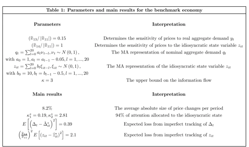
See Table 1 for the parameter values of the benchmark economy. The ratio (ˆπ13/|πˆ11|)

determines the sensitivity of individual prices to real aggregate demand, yt. This is a

stan-dard parameter in models with monopolistic competition. Woodford (2003) recommends a value between 0.1 and 0.15. In the benchmark economy we set (ˆπ13/|πˆ11|) = 0.15. Later

we show how changes in(ˆπ13/|πˆ11|) affect the solution.

The ratio(ˆπ14/|πˆ11|) determines the sensitivity of individual prices to the idiosyncratic

state variable, zit. Since changes in the value of (ˆπ14/|πˆ11|) have the same effects on

equilibrium as changes in the variance of the idiosyncratic state variable, we normalize (ˆπ14/|πˆ11|) to one and we only calibrate the variance ofzit.

We calibrate the stochastic process for qt using quarterly U.S. nominal GNP data from

1959:1 to 2004:1.23 We take the natural log of the data and detrend the data by fitting a second-order polynomial in time. We then estimate the equation qt=ρqt−1+νt, whereqt

is 100 times the deviation of the natural log of nominal GNP from its fitted trend. The estimate of ρthat we obtain is, after rounding off, 0.95 and the standard deviation of the error term is 1. This implies the moving average representation qt = P∞_l=0ρlνt−l. Since

with geometric decay shocks die out after a very large number of periods and computing time is fast increasing with the number of lags, we approximate the estimated process by a process that dies out after twenty periods: qt=P20l=0alνt−l,a0 = 1 and al =al−1−0.05,

for all l= 1, ...,20.24

We calibrate the stochastic process for zit so as to make the model match the average

absolute size of price changes in the data. Recall that Bils and Klenow (2004)find that the medianfirm changes its price every 4.3 months. Furthermore, Klenow and Kryvtsov (2004)

2 3

The source are the National Income and Product Accounts of the United States.

2 4

For the benchmark parameter values, we also solved the model without applying the approximation. We setqt=P80_l=0ρlνt−l. While computing time was many times larger, the results were affected little.

find that, conditional on the occurrence of a price change, the average absolute size of the price change is 13.3% or 8.5% (depending on whether sales are included or excluded). We know from the analytical solution that a larger variance of the idiosyncratic state variables makes the aggregate price level more sticky. We also know that under rational inattention compared to perfect information a larger variance of the idiosyncratic state variables is required to generate a given average absolute size of price changes. We take a conservative approach and choose the standard deviation ofzitsuch that the average absolute size of price

changes under perfect information is 8.5% per period.25 _{This yields a standard deviation}

of zit that is ten times the standard deviation of qt.26

We set the parameter that bounds the information flow to κ = 3 bits. Our choice is motivated by two considerations. First,κ= 3is sizable compared to the amount of uncer-tainty in the model. Iffirms in the model wanted to, they could track aggregate conditions extremely well.27 Second, with this value of κ the model predicts a negligible difference between the price set by afirm under rational inattention and the profit-maximizing price. Wefind this prediction realistic.

Table 1 and Figures 1-2 summarize the results for the benchmark economy. The average absolute size of price changes is 8.2% per period. Firms allocate 94% of their attention to idiosyncratic conditions. This optimal allocation of attention implies the following price setting behavior. Figure 1 shows the impulse response of the price set by firm i to an innovation in the idiosyncratic state variablei. Comparing the price reaction under rational inattention (the line with squares) to the price reaction under perfect information (the line with points), we see that under rational inattention the price reaction to idiosyncratic shocks is almost as strong and fast as under perfect information. The line with crosses is the impulse response of the price set byfirmito noise in the signal concerning idiosyncratic conditions.

Figure 2 shows the impulse response of the price set byfirmito an innovation in nominal 2 5

Recall that one period in the model is one quarter.

2 6

We assume the same rate of decay in thezitprocess as in theqtprocess.

2 7

To illustrate this point, consider a simple example. Suppose that qt was a white noise process with variance 10, which is the variance ofqt in the data. Then allocating 3 bits of informationflow to tracking

aggregate demand. Comparing the price reaction under rational inattention (the line with squares) to the price reaction under perfect information (the line with points), we see that under rational inattention the price reaction to nominal shocks is dampened and delayed. Note that, since all firms choose the same stochastic process for the signal, the line with squares is also the impulse response of the aggregate price level to an innovation in nominal aggregate demand. The aggregate price level responds weakly and slowly to innovations in nominal aggregate demand. The reasons are the following. Since idiosyncratic condi-tions are more variable than aggregate condicondi-tions,firms allocate most of their attention to idiosyncratic conditions. In addition, there is the feedback effect. When firms pay little attention to aggregate conditions, the aggregate price level moves little and thereforefirms find it optimal to pay even less attention to aggregate conditions. As a result, the equilib-rium aggregate price level under rational inattention differs markedly from the equilibequilib-rium aggregate price level under perfect information. Finally, the line with crosses in Figure 2 is the impulse response of the price set by an individualfirm to noise in the signal concerning aggregate conditions.28

The effect of an innovation in nominal aggregate demand on real aggregate demand equals the difference between the perfect-information impulse response in Figure 2 and the rational-inattention impulse response in Figure 2. It is apparent that the real effect of an innovation in nominal aggregate demand is persistent.

Figures 3-4 show simulated price series. Figure 3 shows a sequence of prices set by an individual firm under rational inattention (diamonds) and the sequence of prices that the firm would have set if it had had perfect information (crosses). Firms in the bench-mark economy track the profit-maximizing price extremely well. Figure 4 shows sequences 2 8_{The reader interested in the impulse response of inflation to an innovation in nominal aggregate demand}

should note the following. In the benchmark economy, the peak response of inflation occurs on impact. Below we conduct experiments in which the impulse response of the aggregate price level becomes more dampened and delayed than in the benchmark economy. In these experiments, the impulse response of inflation becomes hump-shaped. See the experiment with a larger variance of the idiosyncratic state variables (section 6.3) and the experiment with more strategic complementarity in price setting (section 6.4). We read the evidence from structural VARs as indicating clearly that the aggregate price level responds slowly to a monetary policy shock. We read the evidence as less conclusive regarding whether the impulse response of inflation to a monetary policy shock is hump-shaped (see Uhlig (2005)).

of aggregate price levels. The equilibrium aggregate price level under rational inattention (diamonds) differs markedly from the equilibrium aggregate price level under perfect infor-mation (crosses). The reason is the optimal allocation of attention in combination with the feedback effect.

In the benchmark economy, prices react fast and by large amounts to idiosyncratic shocks, but prices react only slowly and by small amounts to nominal shocks. Thus the model can explain why individual prices change frequently and by large amounts and, at the same time, the aggregate price level responds slowly to monetary shocks. To match the large average absolute size of price changes observed in the data, idiosyncratic shocks in the model must have a large variance or must be very important for pricing decisions. This in turn implies thatfirms in the model allocate most of their attention to idiosyncratic conditions.

We turn to examining how changes in parameter values affect the optimal allocation of attention and the dynamics of the economy.

6.2

Increasing the variance of nominal aggregate demand

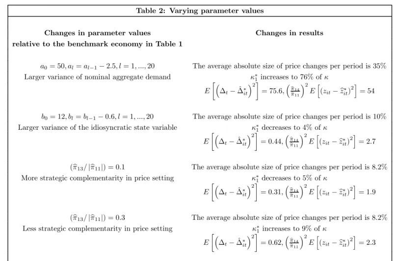
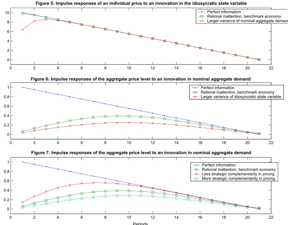
In Table 2 and Figure 5 we show what happens when the variance of nominal aggregate de-mand increases. Firms reallocate attention to aggregate conditions away from idiosyncratic conditions (κ∗₁ increases). Firms track both aggregate and idiosyncratic conditions less well. Profits decrease. The real effects of changes in nominal aggregate demand increase. The fall in profits suggests that costs of aggregate instability in the real world may be due to the fact that aggregate instability makes thefirms’ tracking problem more difficult.

These predictions differ from the Lucas (1973) model. In the Lucas model, an increase in the variance of nominal aggregate demand implies that prices thatfirms observe in their markets become more precise signals of nominal aggregate demand and less precise signals of idiosyncratic conditions. Therefore firms in the Lucas model track nominal aggregate demand better and idiosyncratic conditions worse. The real effects of changes in nominal aggregate demand become smaller.

6.3

Increasing the variance of the idiosyncratic state variables

In Table 2 and Figure 6 we show what happens when the variance of the idiosyncratic state variables increases. Firms reallocate attention to idiosyncratic conditions away from aggre-gate conditions (κ∗₁decreases). Firms track both idiosyncratic and aggregate conditions less well. The reaction of the aggregate price level to a nominal shock becomes more dampened and delayed.

The model predicts thatfirms operating in more variable idiosyncratic environments al-locate less attention to aggregate conditions, and therefore respond more slowly to aggregate shocks. This result is consistent with the empirical finding of Bils, Klenow and Kryvtsov (2003) according to which firms that change prices relatively frequently react more slowly to monetary policy shocks thanfirms that change prices relatively infrequently. Thefinding of Bils, Klenow and Kryvtsov is difficult to reconcile with other models of sticky prices.

The reader may wonder whether these predictions continue to hold in a model with an endogenousκ. Suppose thatfirms can choose the informationflow,κ, facing an increasing, strictly convex cost function,C(κ). Now consider again the effects of increasing the variance of the idiosyncratic state variables. The marginal value of information about idiosyncratic conditions increases. Thereforefirms choose a higherκand the marginal cost of information increases. This implies that the marginal value of information about aggregate conditions has to increase as well — the information flow allocated to aggregate conditions has to fall. Hence, both idiosyncratic and aggregate conditions get tracked less well.

6.4

Changing the degree of strategic complementarity in price setting

The third and fourth example in Table 2 and Figure 7 show what happens when the ratio (ˆπ13/|πˆ11|)changes.29 As(ˆπ13/|πˆ11|)decreases, the impulse response of the aggregate price

level becomes more dampened and delayed. The reason is the following. Under rational inattention, the aggregate price level is less variable than nominal aggregate demand. Thus decreasing (ˆπ13/|πˆ11|) lowers the variance of ∆t =

³

1₋ ˆπ13

|ˆπ11|

´

pt+ _|ˆπ_ˆπ13_11|qt. Firms react by

2 9_{It is common in the literature to refer to the ratio (ˆπ13/}

|π11ˆ _|) as a measure of the degree of strategic complementarity in price setting, where a smaller value of (ˆπ13/_|ˆπ11_|) corresponds to a larger degree of strategic complementarity in price setting.

reallocating attention to idiosyncratic conditions away from aggregate conditions.

6.5

The e

ff

ects of serial correlation

Decreasing the serial correlation of nominal aggregate demand (holding constant its vari-ance) leads to a fall in profits, because the firms’ tracking problem becomes more difficult. This suggests that there is a payoff from “interest rate smoothing” by central banks. We obtained ambiguous predictions concerning the effect of a decrease in the serial correlation of nominal aggregate demand (holding constant its variance) on the allocation of attention. We found that the marginal return from allocating attention to aggregate conditions may go up or down. The reason is that decreasing the serial correlation of nominal aggregate de-mand makesfirms track aggregate conditions less well (for a given allocation of attention), but also lowers the improvement in tracking that can be achieved by reallocating attention to aggregate conditions.30

6.6

Optimal signals

We always verify numerically that there exist signals of the form (51)-(52) that have the property (53)-(54). Figures 8 and 9 present optimal signals for the benchmark economy, by plotting the parameters of the moving average representations of∆t,εit,zit and ψit. A

common assumption in the literature is that signals have the form “true state plus i.i.d. noise”. We always find optimal signals that have the structure “true state plus a moving average noise process”. However, only in some cases we find optimal signals that have the structure “true state plus i.i.d. noise”. For example, the optimal idiosyncratic signal depicted in Figure 9 has the form “true state plus i.i.d. noise”, but the optimal aggregate signal shown in Figure 8 does not.31

3 0

We obtained the same results when we changed the serial correlation of the idiosyncratic state variables.

3 1

Note that optimal signals are not unique. For example, applying any one-sided linearfilter to the signals depicted in Figures 8 and 9 yields new optimal signals. The reason is that applying a one-sided linearfilter changes neither the conditional expectations computed from the signals nor the informationflow.

7

Conclusions and further research

That individual prices move frequently and by large amounts in the data does not imply that the aggregate price level must react fast to monetary policy shocks. When idiosyncratic conditions are more variable or more important than aggregate conditions, rationally inat-tentivefirms optimally allocate more attention to idiosyncratic conditions than to aggregate conditions. As a result, prices react fast and by large amounts to idiosyncratic shocks, but prices react only slowly and by small amounts to nominal shocks. Innovations in nominal aggregate demand have persistent real effects.

In standard sticky price models, frequent and large price changes imply afast response of the aggregate price level to nominal shocks. In our model, frequent and large price changes imply a slow response of the aggregate price level to nominal shocks. The same empirical observation on the frequency and size of individual price changes leads to the opposite aggregate prediction. Therefore our model can simultaneously explain the micro and the macro evidence on consumer prices.

Our model makes several testable predictions that we plan to compare to data. For ex-ample, according to the model,firms operating in more variable idiosyncratic environments react more slowly to nominal shocks.

The model can be extended in a variety of directions. For example, the model in its current form abstracts from physical costs of repricing. This implies that prices in the model change every period. It would be interesting to add menu costs. This is likely to increase the real effects of nominal disturbances even further.32

Furthermore, it will be interesting to develop a richer general equilibrium model with rational inattention and compare its predictions to, for example, Christiano, Eichenbaum and Evans (2005), Altig, Christiano, Eichenbaum and Linde (2005) and Smets and Wouters (2003).

3 2

See Dotsey, King and Wolman (1999) and Golosov and Lucas (2005) for general equilibrium models with menu costs.

A

Quantifying information

fl

ows

This appendix introduces the tools that we use to quantify information flows. We borrow the tools from Shannon’s (1948) information theory. For a textbook on information theory, see Cover and Thomas (1991). For an application in economics, see Sims (2003).

In economics the payoffof a decisionmaker often depends on the realization of a random variable. One can quantify the uncertainty by using the concept ofentropy. The entropy of a random variable is a measure of the uncertainty of the random variable. The entropyH(X) of a random variableX with density function p(X) is defined byH(X) = ₋E[log₂p(X)]. Entropy is measured in bits. For example, the entropy of a normally distributed random variableX with varianceσ2 is

H(X) = 1

2log2

¡

2πeσ2¢.

In this simple example, entropy is a strictly increasing function of the variance.33

The definition of entropy extends to random vectors. In the definition of entropy, sim-ply replace the density function by the joint density function. For example, apsim-plying the definition of entropy to a set of random variablesX1, ..., XT that have a multivariate normal

distribution with covariance matrix ΩXX yields

H(X1, ..., XT) =

1

2log2[(2πe)

T _detΩ

XX]. (59)

The entropy of the random vector depends on the number of random variables and on their covariance matrix. A larger determinant of the covariance matrix implies a larger entropy. For given variances, the entropy is largest when the random variables are uncorrelated.

In economics a decisionmaker often observes a random vector that is correlated with the random vector of interest. One can quantify the conditional uncertainty by using the concept of conditional entropy. For example, suppose that a decisionmaker is interested in X1, ..., XT and observes Y1, ..., YT, where X1, ..., XT and Y1, ..., YT have a multivariate

normal distribution with covariance matrix Ω. Then the entropy of X1, ..., XT conditional

3 3_{The definition of entropy can be derived from axioms — requirements that a “reasonable” measure of}

uncertainty should satisfy (see e.g. Ash (1990)). Moreover, entropy arises as the answer to a number of natural questions in communication theory and statistics (see e.g. Cover and Thomas (1991)).

on Y1, ..., YT is H(X1, ..., XT |Y1, ..., YT) = 1 2log2{(2πe) T _det[Ω XX−ΩXYΩ−Y Y1ΩY X]}. (60)

The expression in square brackets is the covariance matrix of X1, ..., XT conditional on

Y1, ..., YT.

Now one can quantify the amount of information that one random vector contains about another random vector. Mutual information is the reduction in the uncertainty of one random vector due to the knowledge of another random vector. The mutual information betweenX1, ..., XT and Y1, ..., YT is

I(X1, ..., XT;Y1, ..., YT) =H(X1, ..., XT)−H(X1, ..., XT |Y1, ..., YT). (61)

It is also straightforward to quantify the informationflow between stochastic processes. Let X1, ..., XT denote the first T elements of the stochastic process {Xt}. Let Y1, ..., YT

denote the first T elements of the stochastic process _{Yt}. The processes {Xt} and {Yt}

can be vector processes. The informationflow between the processes_{Xt}and{Yt} can be

defined by

I(_{Xt};{Yt}) = lim

T→∞ 1

TI(X1, ..., XT;Y1, ..., YT). (62)

The information flow between stochastic processes is the average amount of information per unit of time that one stochastic process contains about another stochastic process. The limit in (62) exists when the processes _{Xt}and {Yt} are jointly stationary.

In the Gaussian case, an analytical expression exists for the informationflow. If_{Xt}and

{Yt}are univariate, jointly stationary, jointly Gaussian processes with absolutely summable

autocovariance matrices then

I(_{Xt};{Yt}) =− 1 4π π Z −π log₂[1_−CX,Y(ω)]dω, (63)

where_CX,Y (ω)is the coherence between the processes{Xt}and {Yt}at frequency ω. This

follows from equations (59)-(62) and the asymptotic properties of determinants of Toeplitz matrices. See Cover and Thomas (1991, pp. 273-274), Gray (2002, pp. 62-63) or Sims (2003). Note that the coherence lies between zero and one, 0_≤CX,Y (ω) ≤1 for all ω. It

B

Information

fl

ow constraint in the white noise case

Assumptions (10)-(11) imply

I(_{Pt},{Yt},{Zit};{sit}) =I({pt},{yt};{s1it}) +I({zit};{s2it}).

This general result is proved below. See Lemma 2. Furthermore, equations (26)-(27) imply that_{pt} and {yt} can be calculated from{∆t} and vice versa. It follows that

I(_{pt},{yt};{s1it}) =I({∆t};{s1it}).

The signal concerning aggregate conditions is given by equation (28). Equation (63) implies that I(_{∆t};{s1it}) =− 1 4π π Z −π log₂[1_−C∆,s1i(ω)]dω,

where _C∆,s1i(ω) is the coherence between the processes {∆t} and {s1it} at frequency ω. The processes _{∆t} and {s1it} are white noise processes. Therefore the coherence simply

equals the squared correlation coefficient and

I(_{∆t};{s1it}) =− 1 2log2 ¡ 1₋ρ2_∆,s1i¢. Using (28) yields I(_{∆t};{s1it}) = 1 2log2 µ σ2_∆ σ2 ε + 1 ¶ .

The same arguments yield

I(_{zit};{s2it}) = 1 2log2 Ã σ2_z σ2 ψ + 1 ! .

The informationflow constraint becomes 1 2log2 µ σ2 ∆ σ2 ε + 1 ¶ +1 2log2 Ã σ2_z σ2 ψ + 1 ! ≤κ.

C

Proof of lemma 1

When the profit function is given by equation (18), the expected discounted sum of profits equals E "_∞ X t=1 βtπ(P_it∗, Pt, Yt, Zit) # = E "_∞ X t=1 βtπ˜(p∗_it, pt, yt, zit) # = E "_∞ X t=1 βtπ˜ ³ pf_it, pt, yt, zit ´# −E "_∞ X t=1 βt|πˆ11| 2 ³ pf_it−p∗_it ´2# ,

where the second equality follows from equation (21). The difference between the perfect information price (20) and the imperfect information price (19) equals

pf_it−p∗_it =pf_it−Ehpf_it|st_ii.

The joint normality ofpf_it andst_i =_{s1_i, si2, ..., sit}implies that the conditional expectation

equals the linear projection. Furthermore, the joint stationarity ofnpf_itoand_{sit}in

combi-nation with assumption (13) implies that the linear projection coefficients are independent of t

pf_it−p∗_it=pf_it−[µ+α(L)sit],

whereµ is a constant andα(L) is an infinite order vector lag polynomial. Hence,pf_it−p∗_it

follows a stationary process andE

·³

pf_it−p∗_it

´2¸

is independent oft. Equation (41) follows.

D

Proof of lemma 2

First, since _{Pt},{Yt},{Zit} can be calculated from {pt},{yt},{zit} and vice versa, we

have

I(_{Pt},{Yt},{Zit};{sit}) =I({pt},{yt},{zit};{sit}).

Applying the definition of information flow (62) yields

I(_{pt},{yt},{zit};{sit}) = lim T→∞ 1 TI ¡ pT, yT, z_iT;sT_i ¢, where pT _{≡ (p} 1, . . . , pT), yT ≡(y1, . . . , yT), ziT ≡ (zi1, . . . , ziT) and sTi ≡ ¡ s1 i, si2, . . . , siT ¢ . Mutual information equals the difference between entropy and conditional entropy

See equation (61). Conditional entropy equals

H¡pT, yT, zT_{i |}sT_i ¢=H¡pT, yT, zT_i , sT_i ¢₋H¡sT_i¢.

See, for example, Cover and Thomas (1991), p. 230, equation (9.33). We arrive at

I¡pT, yT, z_iT;sT_i ¢=H¡pT, yT, z_iT¢₋H¡pT, yT, z_iT, sT_i¢+H¡sT_i ¢.

Assumption (10) implies

I¡pT, yT, z_iT;sT_i ¢=H¡pT, yT, z_iT¢₋H¡pT, yT, z_iT, sT_1i, sT_2i¢+H¡sT_1i, sT_2i¢.

The entropy of independent random variables or independent random vectors equals the sum of the entropies. See, for example, Cover and Thomas (1991), p. 232, equation (9.59). Therefore assumption (11) implies

I¡pT, yT, zT_i ;sT_i ¢ = H¡pT, yT¢+H¡zT_i ¢₋H¡pT, yT, sT_1i¢₋H¡zT_i , sT_2i¢

+H¡sT_1i¢+H¡sT_2i¢.

The last equation can also be expressed as

I¡pT,